1
Study of Turbulent Flows through A Conduct Square Section with A 90 °
Elbow
Rabia FERHAT (1), Leila MERAHI (2), Bouabdellah ABED (3) and Ali Belabdi 1University des Sciences et de la Technologie d’ORAN, Faculté de Génie-Mécanique
Email : (1) [email protected] Abstract
In the present work, a numerical simulation of turbulent flows, three-dimensional incompressible of a fluid through a 90° elbow square section, using a computing code ANSYS CFX that models the characteristics of the flow of fluids in complex geometries and using structured meshes. The general structure of the flow (hydrodynamic fields as well as the parameters of the turbulence) has been obtained for the Geometry considered, we have tested the performance of two models of ε turbulence and ω OSH, it proves that the model ω SST is more efficient meadows of wall that the k-ε model. the study confirms the existence of secondary flows to the interior and after the elbow. In fact, the flows at the level of Elbow are characterized by the presence of cells counter-rotating responsible on the disruption of the flow.
Key words: Elbow, Turbulence, Secondary flow, counter - rotating cells. 1-Intoduction
Square curved pipes (elbows) are often used in the installation of energy and power, such as fuel supplies, exhaust systems, and many others. In flows through straight and rectangular pipes, the pressure fields in individual cross-sections exhibit a considerable degree of homogeneity. However, in flows through installed pipes and bend conduits, speed and pressure fields are highly complex. Inertial forces, particularly in the bend, cause large pressure gradients in the direction from the inner wall to the outer wall. The vortex zones which form directly before and after the turn are the cause of so-called secondary flows in the area of curvature and additional pressure losses. Numerous experimental and numerical studies have been carried out to characterize these complex flows. Lyne [1] is one of the first to treat the case of a flow induced by a pulsation in a curved pipe. Humphrey [2], Enayet, [3] Azzola [4] and Cheah [5] used the LDA (Doppler Anemometry laser) to measure the velocity field and flow visualization in a 90 ° elbow of square cross section. The covides [6] used hot-wire anemometry for measurements in curved conduits. Munch and Mait [7] evaluated the influence of the aspect ratio of the section on compressible and three-dimensional turbulent flows by Large Scale Simulation, developing in curved conduits of rectangular section. Sugiyama and Hitomi [8] used the Reynolds algebraic constraint model (ARSM) to analyze three-dimensional turbulent flow in a 180 ° bend. Jiann.C, Jyh.T [9], A. Ono, N. Kimura [10] and Jiann-Cherng Chu [11] experimentally and numerically studied flow characteristics in curved rectangular microchannels. The study of turbulent flows in curved conduits is an open problem presenting important technological stakes and remains motivating for part of the research on fluid mechanics.
2. Mathematical model and numerical method
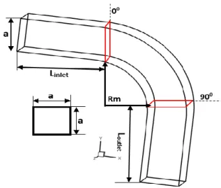
The geometry considered is a 90 ° elbow with a square cross-section similar to that used by Sudo.K, Sumida.M, Hibara.H [12] concerning the square-section elbow for turbulent flows (Fig.1).
2
Figure 1: Elbow 90° with square section Table 1: The dimensions of the elbow
dimensions Length (mm) Ray (mm)
Before elbow (Linlet) 1600 -
In the elbow (Rm) - 160
after the elbow (Loutlet) 1600 -
Elbow section (a) 80 -
The Turbulent flow is considered air (at 298k), all thermophysical properties are assumed to be constant. The numerical simulations were performed using commercial codes CFD ANSYS CFX (versions 14) to solve our problem. These codes use the finite volume method to solve the set of partial differential governing equations. The governing equations consist of equations of transport and momentum, continuity and energy. Equations for constant flux expressed using a Reynolds averaged Navier-Stokes (RANS) method can be formulated as follows:
A. Equation of continuity 0 j j x u (1)
B. Equation of movement quantity
i j i j j i j j uu g x x P U x U ' ' 2 (2) C. Equation of Energy
' '
2 2 p j j j j j t u x x T Cp T U x (3) All these equations can be written in the following general form:
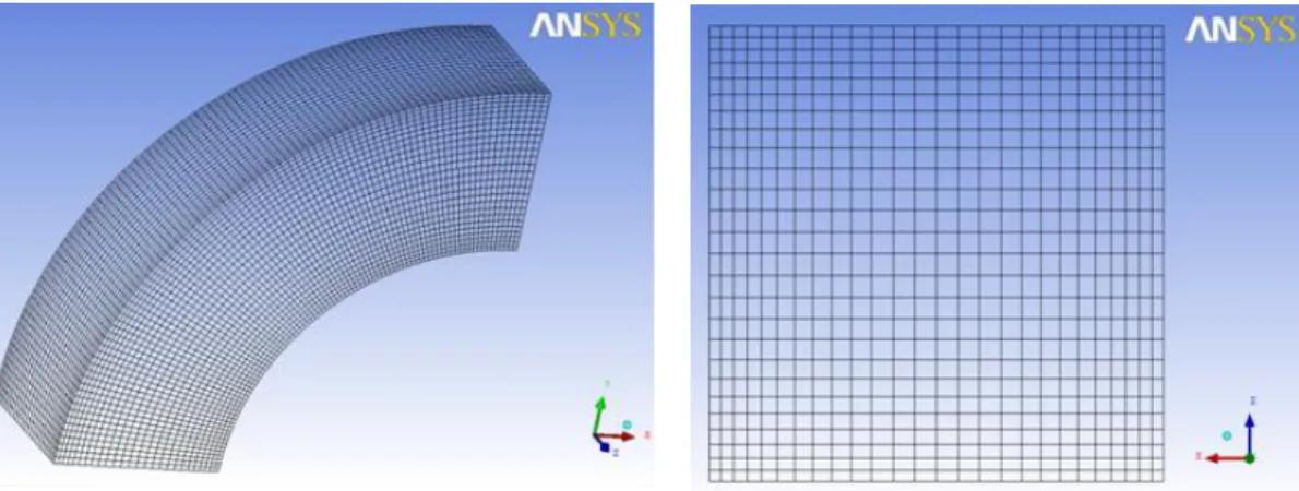
S x x x u j j j (4) 3. MeshingWe use uniform (structured) hexahedra grids for the k-ε and non-uniform turbulence model for kω-SST (Fig.2), (Fig.3). In the present study, non-uniform structured hexahedral cells are created with a fine mesh near the walls using the ANSYS ICEM mesh generation software. This is done to provide a sufficiently grouped mesh near the walls of the elbow (Fig. 3). Several meshes were tested to ensure that the solution was independent of the mesh. Therefore, the mesh 1 (254754 cells) will be retained for the study of the air flow in the present work.
3
Figure 2 : The mesh for the turbulence model k-ε
Figure 3 : The mesh for the k-ω SST turbulence model
4. Results and discussion
In order to validate our calculation code comparisons were made between the experimental results of Sudo K, Sumida M, Hibara H [12] and the numerical results of our present study. FIGS. 4, 5 and 6 show comparisons between the obtained numerical results of the two models used k-ε, k ω-SST and the experimental results corresponding to the article [13].
Figure 4 : Comparison of speed profiles for = 30° and Z/Dh = 0
Figure 5 : Comparison of speed profiles for = 6° and Z/Dh = 0
4
Figure 6 : Comparison of speed profiles to distance X/Dh = 1 and Z/Dh = 0
We show in figures 4, 5 and 6 the variation in the speed ratio (U/Vc) as a function of Y/a for = 30˚, = 60˚ and X/Dh=1.
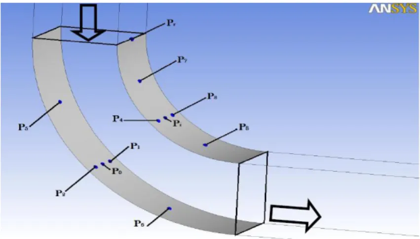
Figure 7 : Pressure measurement points Table 2: Comparison of experimental and numerical measured pressure differences
Reelbow
P01(Pa) P02(Pa) Pi3(Pa) Pi4(Pa) P24(Pa)
Exp Num Exp Num Exp Num Exp Num Exp Num 42290 0.69 0.57 0.49 0.29 0.88 0.62 0.98 0.63 73.58 74.23 74888 2.92 1.86 2.92 0.57 1.96 0.98 2.45 1.17 173.64 172.58 92184 1.08 1.13 0.98 0.62 1.08 0.25 1.57 0.77 262.91 261.92 125263 1.96 1.85 0.5 1.47 0.05 -0.88 0.00 -0.92 465.98 478.49
Figure 8 shows the differences in pressures at the ends of the elbows (φ= 22.5°, 45°, 67.5°) between certain selected points of the surface of the elbow side (P0, Pi, P1, P2, P3, P4, P5, P6, P7, P8). The differences in pressures ΔP01,ΔP02 ,ΔPi3,ΔPi4 ,ΔP24 are indicated in (Tab.2).
5 4.1 The Model k-ε
Figure 8 : Pressure field at median plane Z = 0 for
different angles Figure 9 : Pressure profiles at the median plane Z = 0 for different angles
Figures (8), (9) show the pressure field and profiles as a function of the radial position Z = 0 and also the contours of pressure in the median plane for different angles.
An increase in the pressure of the inner wall towards the outer wall of the elbow is due to the concentration of the flow. It can be said that the pressure gradient with respect to the radial direction is maximal at the angle 60 ° approximately.
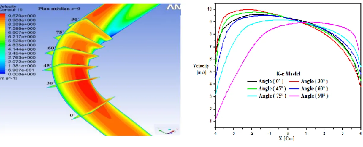
Figure 10 : Speed field at the median plane Z = 0 for different angles
Figure 11 : Speed profiles at the median plane Z = 0 for different angles
The velocity field in the elbow moves from the center to the inner wall of the elbow in the range of 0 ° to 30 ° because of the flow that takes the trajectory of the elbow and in the range 30° to 90°, The flow deflects from the inner wall to the outer wall due to the inertial forces which define the separation of the flow (Fig 10) and (Fig 11).
6
Figure12 : Field of kinetic energy at the median plane Z = 0 for different angles
Figure 13 : Kinetic energy profiles at the median plane Z = 0 for different angles
The relatively low values of the turbulent kinetic energy upstream and in the first half of the elbow reflect the fact that the flow is virtually potential, except very close to the walls or evolves the viscous flow of the thin boundary layers. It is confirmed that the turbulent kinetic energy is concentrated near the side walls of the elbow because of the viscous boundary layer (Fig. 12), (Fig. 13)
4.2 Comparison of model k-ε and SST
𝜑 = 60° 𝜑 = 75°
𝜑 = 90° X=4Dh
Figure 14: Comparison between the velocity vectors obtained by the k-ε and SST models
Figure (14) shows the model superiority SST with respect to the standard model k-ε. Indeed, with the SST model we see that the secondary flow consists of two pairs of contra rotating cells in the square-section pipe, whereas these do not appear when using the standard model k-ε. We would like to point out that these pairs of contra rotating cells have been reported in several experimental and numerical studies.
7 5. Conclusion
The objective of the work presented is to analyze and study the behavior of a turbulent air flow through a square pipe with a 90 ° elbow and an understanding of the physical mechanisms governing the flows (K-ε, k-ω SST) on the dynamic field (pressure, velocity, turbulent kinetic energy) in this type of pipe, by focusing on the influence of the curvature. The study of secondary flows gives an idea of the complexity of the flows in the organs causing singular pressure drops, for simplicity we will reason in the case of an elbow. The SST model is well provided for the recirculation zone, whereas the k-ε model is more efficient in the median area of the elbow. Références [1] [2] [3] [4] [5] [6] [7] [8] [9] [10] [11] [12] [13]
Lyne.H. Unsteady viscous flow in a curved pipe. J fluid meeh.1970. Vol 45. pp.13-31. Humphrey.C, Taylor.K et Whitelaw.H. Laminar flow in a square duct of strong curvature. J Fluid Mech. 1977. Vol 83. pp.509-527.
Enayet.M, Gibsen.M, Taylor.P, Yianneski.M. Laser-doppler measurements of laminar and turbulent flow in a pipe bend. Int.1. Heat Fluid Flow. 1982. Vol. 3. pp. 213-219. Chang.M, Humphrey.C. et Modavi.A. Turbulent flow in a strongly curved U-bend and Downstream tangent of square cross-sections. PhysicoChemical Hydrodynamics. 1983. Vol 4. pp.243-269.
Azzola.J, Humphrey.C, Iacovides.H et Launder B.E. Developing turbulent flow in a U-bend of circular cross section: measurement and computation., transactions of the Asme, Journal of fluid engineering. 1986. Vol 08. pp. 214-221.
Cheah.C, Iacovides.H, Jackson.C, Li.H et Launder.E. LDA Investigation of the flow development through rotating U ducts. ASME. 1994. paper 94-GT.226.
Iacovides.H, Launder.E, Loizou.A et Zha.H. Turbulent boundary layer development around a square sectioned V-end: measurements and computation. J. Fluid Eng. 1990 Vol 112. pp. 409-415.
Munch.C, Hébrard.J et Métais.O. Large-eddy simulation of turbulent flow in curved and S-shape ducts. ereoftae Kluwer. 2004. pp. 527-536.
Sugiyama.H et Hitomi.D. Numerical analysis of developing turbulent flow in 1800 bend tube by an algebraic Reynolds stress model. Int. J. Numer. Meth. Fluids. 2005. Vol47. pp. 1431-1449.
Jiann.C, Jyh.T. Experimental and numerical study on the flow characteristics in curved rectangular micro channels. Applied Thermal Engineering. 2010. Vol30. pp.1558-1566. Ono.A, Kimura.N. Influence of elbow curvature on flow structure at elbow outlet under high Reynolds number condition. Nuclear Engineering and Design. 2011. Vol.241 pp.4409-4419.
Jiangfeng.G, Jun.C. Viscous dissipation effect on entropy generation in curved square microchannels. Energy. 2011. Vol36. pp.5416-5423.
Sudo.K. Une étude expérimentale d'un écoulement turbulent stationnaire dans un coude de section carrée. Experiments in Fluids. 2001. Vol. 30, pp. 246-252.