Static Analysis and Stochastic Search for Reachability Problem

HAL Id: hal-01951251

https://hal.archives-ouvertes.fr/hal-01951251

Submitted on 11 Dec 2018

HAL is a multi-disciplinary open access

archive for the deposit and dissemination of

sci-entific research documents, whether they are

pub-lished or not. The documents may come from

L’archive ouverte pluridisciplinaire HAL, est

destinée au dépôt et à la diffusion de documents

scientifiques de niveau recherche, publiés ou non,

émanant des établissements d’enseignement et de

Static Analysis and Stochastic Search for Reachability

Problem

Xinwei Chai, Tony Ribeiro, Morgan Magnin, Olivier Roux, Katsumi Inoue

To cite this version:

Xinwei Chai, Tony Ribeiro, Morgan Magnin, Olivier Roux, Katsumi Inoue. Static Analysis and

Stochastic Search for Reachability Problem. 9th Workshop on Static Analysis and Systems Biology

(SASB 2018), Aug 2018, Freiburg, Germany. �hal-01951251�

Static Analysis and Stochastic Search for

Reachability Problem

Xinwei Chai, Tony Ribeiro, Morgan Magnin, Olivier Roux

Laboratoire des Sciences du Num´

erique de Nantes, 1 rue de la No¨

e,

44321 Nantes, France

Katsumi Inoue

National Institute of Informatics, 2-1-2 Hitotsubashi, Chiyoda-ku,

Tokyo 101-8430, Japan

Abstract

This paper focuses on a major improvement on the analysis of reacha-bility properties in large-scale dynamical biological models. To tackle such models, where classical model checkers fail due to state space explosion led by exhaustive search. Alternative static analysis approaches have been proposed, but they may also fail in certain cases due to non-exhaustive search. In this paper, we introduce a hybrid approach ASPReach, which combines static analysis and stochastic search to break the limits of both approaches. We tackle this issue on a modeling framework we recently introduced, Asynchronous Binary Automata Network (ABAN). We show that ASPReach is able to analyze efficiently some reachability properties which could not be solved by existing methods. We studied also various cases from biological literature, emphasizing the merits of our approach in terms of conclusiveness and performance. keyword: Model checking, Reachability problem, Asynchronous Binary Automata Network, Local Causality Graph, Heuristics, Answer Set Programming.

1

Introduction

With increasing quantities of available data provided by new technologies, e.g. DNA microarray [22], there is a growing need for expressive modelings and their related high-performance analytic tools. Among them, works on concurrent systems have been of interest in systems biology for over a decade [4, 5, 35]. If model validation is a major concern, one of the main challenges nowadays is predicting the behavior of these systems.

Reachability problem on formal models is a critical challenge where both validation problems (whether the model satisfies the a priori knowledge) and prediction problems (properties to be discovered) meet. From a formal point of view, numerous biological properties in computational models can be trans-formed to reachability properties. For example, the reachability of state 0/1 of a could represent the activation/inhibition of certain gene or synthesis of a protein, while initial state could represent initial observation in an experiment. If the reachability of a certain state contradicts with the a priori knowledge, one can modify the model and/or design a new experiment to verify whether there is an error in the a priori knowledge or former observation. Also, reachability analysis is of help to medicine design: for example if one wants to prevent the carcinogenesis of a cell (target state), one possible solution is to find the critical pathways towards the target state and design a medicine to cut them in order to keep the cell healthy.

In the domain of model checking, reachability has been of great interest for over 30 years [10, 11]. Various modeling frameworks and semantics in bioin-formatics have been studied: Boolean network [2], Petri nets [23, 14], timed-automata [12, 36]. These approaches rely on global search and thus face state explosion problem as the state space grows exponentially with the number of variables. In [28], it has been shown that the reachability problem of Petri net is exponential time-hard and exponential space-hard, and this conclusion does not change even under some specific conditions [14]. For 1-safe Petri nets, the complexity of reachability analysis is generally PSPACE-complete [8]. Li et al. [20, 21] investigated theoretically the stability, the controllability and the reachability of Switched Boolean Networks, but their method remains compu-tationally expensive; Saadatpour et al. [30] researched only the reachability of fixed points.

To tackle the complexity issue, symbolic model checking [6] based on ordered binary decision diagrams (OBDDs) and SAT-solvers (satisfiability) [1] have been studied over years, but still fail to analyze big biological systems with more than 1000 variables. Bounded Model Checking (BMC) [9] is an efficient approach but generally not complete as its searching depth is limited to a given integer k.

Beside these approaches, abstraction is an efficient strategy to deal with such models of big scale. It aims at approximating the model while keeping the most important parts influencing the reachability. Abstract methods often have better time-memory performance but with a loss of information. They solve usually a simplified version of the original model, i.e. the results from these approaches are not necessarily compatible with all the properties of the original model. While studying reachability problems, the system dynamics is abstracted to static causalities between states and transitions.

We have designed a new discrete modeling framework for a concurrent system [7]: Asynchronous Binary Automata Network (ABAN). In ABAN, we applied the approach developed by Paulev´e et al. [25, 15, 26] to address reachability problem. This approach refers to a static abstraction of the reachability (with an over-approximation and an under-approximation of the real dynamics). It is based on an abstract interpretation: Local Causality Graph (LCG). This

interpretation drastically reduces the searching state-space thus avoids costly global search [27]. However, this pure static analysis is not complete as there are inconclusive cases which can not be decided reachable or not.

Many biological networks are encoded in Boolean style, e.g. [2, 18], because BN is a simple formalism but with strong applicability: discretization in BN is a way to handle the imprecision of a priori knowledge on the model. However BN may be not expressive enough. As to the modeling of the dynamic behavior “a ← 1 at moment t + 1 if b = 1 at moment t”, one has a(t + 1) = b(t) in BN. a always follows the evolution of b but with a potentially unwanted behavior “a ← 0 when b = 0 at moment t”. ABAN models this dynamics as via {b1} → a1

without this redundancy. Besides, BNs are transformable to ABANs, and this property makes our approach applicable to a wider domain (Appendix A).

Our work shares similar concerns but we combine static analysis and bounded model checking. We have developed a heuristic approach PermReach to attack reachability problem [7] which is more conclusive than pure static analysis but time-consuming and still not able to solve reachability problems under certain conditions. In this paper, we propose a hybrid approach ASPReach based on the former LCG reasoning and a non-exhaustive search in the LCG to obtain a more conclusive solution of reachability problems. ASPReach allows one to solve the cases where other static methods fail. Furthermore, it can also solve the reachability of a set of states which to our knowledge has never been done in static way. We assess the value of our contribution using benchmarks on biological examples from the literature.

This paper is organized as follows: Section 2 introduces the formal back-ground and the formalization necessary to the understanding of the work; Sec-tion 3 presents the concrete methods and algorithms composing the whole ap-proach; Section 4 shows the benchmarks evaluating our approach and other alternatives; Section 5 concludes this paper.

2

Formalization

Notations:

ai means automaton a is taking value i;

x :: y is the sequential connector of entities x and y, where x appears just before y;

a.next is the immediate successor of a; a.pred is the immediate predecessor of a.

Boolean Network is a traditional and efficient modeling framework, with many biological networks encoded in BN [18]. To describe the dynamical prop-erties more precisely, Automata Network is introduced [7, 29]. It can be con-sidered as a subset of communicating finite state machines or safe Petri Nets.

Asynchronous Binary Automata Network (ABAN) is a special case of Au-tomata Network. “Asynchronous” implies the update scheme that no more than one automaton can change its value at a time. Asynchronous update scheme makes a trade-off between the biological reality and complexity. From a given

state, biological systems may evolve to multiple future states (e.g. cell differ-entiation), but it is costly to simulate generalized ANs where arbitrary subsets of automata can be updated simultaneously. “Binary” implies that every au-tomaton has exactly two possible states (0, 1). In Appendix A, we show how to transform a Boolean Network into ABAN.

Definition 1 (ABAN). An ABAN is a triplet AB = (Σ, L, T ), where:

• Σ , {a, b, . . .} is the finite set of automata with every component having a Boolean state;

• LS , ∪

a∈Σ{a0, a1} is the set of all local states, L , ×a∈Σ0{a0, a1} is the set

of joint states where Σ0⊆ Σ. Particularly, if Σ0 _{= Σ, L is the set of global}

states.

• T , {A → bi | b ∈ Σ ∧ A ∈ L} is the set of transitions, where A (called

head) is the set of required state(s) for transition tr = A → bi , which

allows to flip b1−ito bi(called body). In other words, transition tr is said

fireable iff A ⊆ s, where s is the current global state.

A local state represents the state of one automaton, e.g. a1, while a global

state represents the joint state of all the automata in the network, e.g. ha0, b1, c0i

where L = {a, b, c}.

Definition 2 (Asynchronous Dynamics). From current global state s, the global state after firing transition tr = A → biis denoted s·tr = s\{b1−i}∪{bi}, where

b1−i∈ s. The state of a certain automaton a is noted (s · tr)[a]. Particularly,

if there is no fireable transition, the next state remains the same as the current state.

To describe the evolution in an ABAN, we use the notion of trajectory. Definition 3 (Trajectory). Given an ABAN AB = (Σ, L, T ) and a global initial state α ∈ L, a trajectory t from α is a sequence of transitions t = tr1 :: · · · ::

tri:: · · · :: trn with tri∈ T and each tri is fireable in (s · tr1· . . . · tri−1). From

α, the global state after firing all transitions of t is (s · tr1· . . . · trn), denoted

s · t.

Definition 4 (State sequence). Given an ABAN AB = (Σ, L, T ) and a global initial state α ∈ L and trajectory t, the state sequence seq = s1:: · · · :: si:: · · · ::

sn with si∈ LS is formed by the updated local states during the trajectory t.

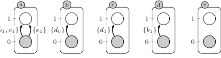
Example 1. Fig. 1 shows an ABAN with initial state α = ha0, b0, c0, d0, e0i

and a possible trajectory is t = {d0} → b1 :: {b1} → d1 :: {d1} → c1 ::

{b1, c1} → a1. After firing the transitions in trajectory t, the state becomes

Ω = s · t = ha1, b1, c1, d1, e0i, and ω = a1 = (α · t)[a]. The state sequence is

a 0 1 b 0 1 c 0 1 d 0 1 e 0 1 {b1, c1} {e1} {d0} {d1} {b1}

Figure 1: An example of ABAN

As to reachability problem, given an ABAN AB = (Σ, L, T ), the joint reach-ability REACH(α, Ω) is formalized as: joint state Ω is reachable iff there ex-ists a trajectory t s.t. α · t = Ω. Partial reachability reach(α, ω) is defined analogously: local state ω = ai is reachable iff there exists a trajectory t s.t.

(α · t)[a] = ai. REACH(α, Ω) and reach(α, ω) take Boolean values True, False

or Inconclusive if it cannot be decided. In Fig. 1, Ω = ha1, b1, c1, d1, e0i or

ω = a1 is reachable from initial state α via trajectory t, i.e. reach(a1) = True

and REACH(α, Ω) = True. In fact, the reachability of a joint state even a global state is equivalent to that of one local state. Given a set of target states {ai, . . . zj}, by adding a new automaton x to Σ, setting its initial state to x0

and adding transition {ai, . . . zj} → x1 to T , REACH(α, {ai, . . . zj}) is thus

equivalent to reach(α, x1). For convenience, we study partial reachabilities in

this paper.

Paulev´e et al. [26] have proposed Local Causality Graph (LCG) to analyze reachability problems statically. LCG abstracts the original problem through an over-approximation (necessary condition) and an under-approximation (suf-ficient condition). It is a very ef(suf-ficient tool as there is no global search and all the operations are bounded in polynomial complexity. However LCG does not guarantee to obtain a result, i.e. some inconclusive instances satisfy the necessary condition and fail sufficient conditions. In this paper, we make use of LCG by removing some elements needed only in multivalued networks, then we try to analyze it more deeply to solve inconclusive cases of binary valued systems. In fact, Didier et al. have shown a technique to transform a multi-valued network to Boolean network [13], which provides us the applicability to multivalued situations.

Definition 5 (LCG). Given an ABAN AB = (Σ, L, T ), an initial state α and a target state ω, LCG l = (Vstate, Vsolution, E) is the smallest recursive structure

with E ⊆ (Vstate× Vsolution) ∩ (Vsolution× Vstate) which satisfies:

ω ∈ Vstate

ai∈ Vstate ⇔ {(ai, solai)|ai∈ α} ⊆ E

solai∈ Vsolution ⇔ {(solai, Va(solai)} ⊆ E

where Vstate⊆ LS is the set of local states, Vsolution ⊆ T is the set of solutions

and Va is the set of required local states of solai.

a1

e1 AND

OR b1 d0 ∅

c1 d1

Figure 2: Visualization of LCG, with the squares representing local states and small circles representing solution nodes. ∅ signifies that there is no need to link any transitions, i.e the former state d0 is in the initial state.

Algorithm 1 describes how to construct an LCG from an ABAN AB = (Σ, L, T ). Starting from a given target state Ls = ω, one can find all the transitions Ts ⊆ T reaching ω and add edges ω → Ts. Then we find all the

heads A of Tsand add edges Ts→ A and replace Ls with A (recursion). Finally,

we update the structure until Ls ⊆ α or there is no transition with body in Ls. Algorithm 1 Construction of LCG

Input: an ABAN AB = (Σ, L, T ), an initial state α, a target state ω Output: LCG l = (Vstate, Vsolution, E)

Initialization: Ls ← {ω}, Vstate← ∅, Vsolution← ∅, E ← ∅

while Ls 6= ∅ do Ls = Ls\Vstate for ai∈ Ls do Ls ← Ls\{ai} if ai∈ α then E ← E ∪ {(ai, ∅)} else

// Choose the transitions reaching ai, i.e. with body a1−i

for sol = A → a1−i∈ T do

Vsolution← Vsolution∪ {sol}

E ← E ∪ {(ai, sol)} Vstate← Vstate∪ A for bj∈ A do E ← E ∪ {(sol, bj)} Ls ← Ls ∪ A Vstate← Vstate∪ Ls

Vsolution← Vsolution∪ ai.next

return (Vstate, Vsolution, E)

Intuitively, when the recursive construction is complete, SLCG is in fact a digraph with state nodes Vstate and solution nodes Vsolution. E consists of the

edges between local state nodes and solution nodes. To access certain local states, at least one of its successor solutions (corresponding transitions from solution nodes) need to be fired; to make one solution node firable, all of its

successor local states need to be satisfied. A recursive reasoning of reachability begins with a state node representing target local state, goes through ai →

solai → bj· · · and ends with initial state (possibly reachable) or a local state

without solution successor (unreachable).

With LCG, it is easy to verify whether their are potential pathways from the target state ω to the initial state α. If there does not exist such a pathway, one can ensure that ω is not reachable from α. [27] explains this local reasoning. Definition 6 (Pseudo-reachability). Given an LCG l = (Vstate, Vsolution, E)

with global initial state α, the pseudo-reachability of node v ∈ Vstate is defined

as reach0(α, v) =      True if v ∈ α

False if v 6∈ α and 6 ∃(s, sol) ∈ E W

(s,sol)∈E(

V

(sol,s)∈Ereach0(α, s)) otherwise

However, pseudo-reachability is named “pseudo” because it is only an over-approximation of reachability, i.e. it reveals a necessary condition of reachability. Example 3. In Fig. 3, reach0_{(l, c}

1) = reach0(l, a1)∧reach0(l, b1) = reach0(l, a0)∧

reach0(l, b0) = True. Both a1and b1are reachable, but they can not be reached

simultaneously. In such LCG, there are two branches, a1 7→ b0 and b1 7→ a0,

the automata a and b involve themselves in different branches, the reachability of a1impedes the reachability of b1 and vice versa.

a 0 1 b 0 1 c 0 1 {a1, b1} {b0} {a0} c1 a1 b0 ∅ b1 a0 _∅ AND Figure 3: Σ = {a, b, c}, T = {{b0} → a1, {a0} → b1, {a1, b1} → c1}, ω = c1

Also, the recursive reasoning does not terminate if there exists cycles in LCG. While computing the pseudo-reachability, self-dependent form reach0(l, ai) =

. . . = reach0(l, ai) will appear. Dealing with cycles becomes inevitable.

Definition 7 (Cycle). In an LCG, a cycle is formed by a sequence of nodes linked as follows: ai→ ◦ → · · · → ◦ → ai

To identify cycles, we search instead Strongly Connected Components (SCC) of size greater than one. Because cycles may interlace and there is no such problem in SCC. In other words, a SCC may contain several nested cycles which connect to each other. [33] shows that the detection of SCCs can be done in O(|V | + |E|) time, with |V | the cardinality of the vertices and |E| the cardinality of the edges. LCG is usually a sparse graph, as in biological systems,

the components mostly interact with only a part of the system, hence the out-degree can be considered of O(1) and the detection of SCCs1 can be done in O(|V |), i.e. linear time.

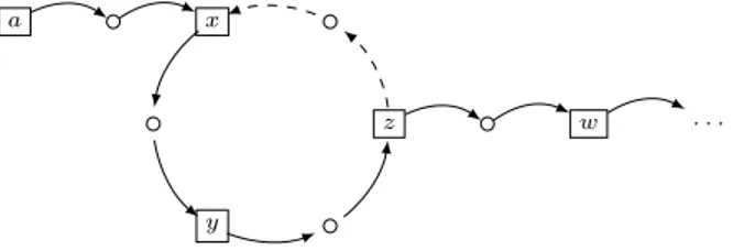
Theorem 1. Given a cycle x → ◦ → · · · → ◦ → x in an LCG, if there is at most one incoming edge to the cycle, the cycle can be removed.

Proof. If there is no incoming edge, the target state y must be in the cycle. The edge y.pred → ◦ → y can be removed, because the reachability of y.pred requires y, but y is the target state, which is never reached before the other local states in the LCG are reached. Thus the transition corresponding to this edge is never fired and the edge can be removed. Similarly, if there is an outside incoming edge a → ◦ → x, a must be the successor of target state y or the target itself, x.pred → ◦ → x can hence be removed.

x

y

z a

w · · ·

Figure 4: LCG l containing cycle x → ◦ → y → ◦ → z → ◦ → x Example 4. In Fig. 4, the pseudo-reachability of a is

reach0(l, a) = reach0(l, x) = reach0(l, y) = reach0(l, z) = reach0(l, x)∨reach0(l, w) To reach x, we need to reach z, but z cannot depend on x as x is already to be reached. Self-dependence appears: x is reachable if x is reachable. Thus edge z → ◦ → x is deleted (dashed line).

Unfortunately, not all cycles are removable via Theorem 1. Example 5 ex-plains the issue.

x

y

z a

Figure 5: x, y, z all have external links, thus none of the links can be discarded

1_{Python3 implementation at https://github.com/alviano/python/blob/master/} rewrite_aggregates/scc.py

Example 5. Cycle x → ◦ → y → ◦ → z → ◦ → x is unbreakable according to Theorem 1, is possesses 3 incoming edges. But with Theorem 2, if OR gates are removed, the cycle can be dealt with. The removal of OR gates is stated in the next section.

Theorem 2. Given a cycle, if it contains no OR gate, all the local states in the cycles are unreachable.

Proof. Suppose an arbitrary cycle C = ai→ · · · bj→ · · · → ai, with → an edge

in the LCG. Note that reach0(α, ai) =⇒ reach0(α, bj) =⇒ reach0(α, bj.next) =⇒

· · · =⇒ reach0_{(α, a}

i). According to the definition of reach0, reach0(α, a) =

True only if ∃ck ∈ C and ck ∈ α. If there exists such ck, C should not

exist as the reasoning stops at ck and does not form a cycle, contradiction.

reach0(α, ai) = reach0(α, bj) = · · · = False.

3

ASPReach Algorithm

In this section, we present the main contribution of this paper, our analyzer ASPReach: an algorithm for checking the reachability of a target local state ω from a global initial state α (which can also be partial) in a given ABAN. How-ever, exhaustive search leads to heavy computation and huge need of memory. The algorithm proposed below tries to overcome those shortcomings by com-bining static analysis and stochastic search into the following hybrid approach.

ASPReach:

• Input: An ABAN AB, an initial state α, a target state ω and a max number of iterations k

• Output: reach(ω) ∈ {False, True, Inconclusive} 1. Construct the LCG l = LCG(AB, α, ω)

2. Try to remove all cycles and prune useless edges from l

3. Try to prove unreachability of ω in l using pseudo-reachability reach0(l, ω) and return False if reach0(l, ω) = False

4. Try at most k times • l0_{← l}

• Simplify each OR gate such that l0_{is a LCG with only AND gates}

• If there remain cycles: – Back to step (iv)

• Generate all trajectory that starts with α in l0 _{using ASP}

5. return Inconclusive

LCG illustrates the causality between necessary transitions to be fired to reach the target state; the tentative of removing cycles simplifies the LCG and keep the reachability unchanged; pseudo-reachability allows one to filter some unreachable cases based on the topology of LCG. The heuristic approach is the core of our algorithm. Stochastic choices avoid combinatorial explosion on different OR Gates. The ASP part searches thoroughly the result but does not traverse the whole state space (ASP solver starts from constraints, finds one consistent order and terminate the search).

Algorithm 2 ASPReach

1: Input: LCG l = (Vstate, Vsolution, E), an integer k

2: Output: reachability r and a trajectory t

3: Compute SCCs, classify them into SCC1(l) with at most 1 incoming edge

and SCC2(l) otherwise

4: // 1) Break all cycles and prune useless branches

5: for each (V_state0 ⊆ Vstate, Vsolution0 ⊆ Vsolution) ∈ SCC1(l) do

6: for each v ∈ V_state0 do

7: if ∃(v, v0) ∈ E, v0 ∈ (Vsolution\ Vsolution0 ) then

8: E ← E\{(v, v00)|v00∈ V0

solution, (v, v00) ∈ E}

9: // 2) remove useless nodes/edges

10: pruned = True

11: while pruned do

12: pruned = False

13: for v ∈ Vstate do

14: if 6 ∃(v, v0) ∈ E then

15: Vstate← Vstate\{v}; E ← E\{(v00, v) ∈ E}

16: E ← E\{(v00, sol) ∈ E|sol ∈ {sol = (A → a) ∈ Vsolution|v ∈ A}}

17: Vsolution← Vsolution\{sol = (A → a) ∈ Vsolution|v ∈ A}

18: pruned = True

19: // 3) Check pseudo-reachability

20: if pseudoReach(l) = False then

21: _{return (False, ∅)} 22: // 4) main search loop

23: for each i in 1 . . . k do

24: l0 = (V_state0 , V_solution0 , E0) ← (Vstate, Vsolution, E)

25: for v ∈ V_state0 do// Treat each OR gates

26: pick a random element (v, v0) ∈ E0

27: E0← E0_{\{(v, v}00_{) ∈ E}0_|v00_{6= v}0_{} with @i ∈ SCC2(l) and i ∈ E}0

28: (r, t) ← ASPsolve(l0)

29: if r = True then return (True, t)

30: _{return (Inconclusive, ∅)}

LCG l as input whose detailed construction is given in Algorithm 1. Lines 4-8 delete all cycles with at most one incoming edge. After removing cycles, the LCG may contain nodes without successor. Such nodes can be pruned since they do not lead to initial state (Line 9-18). This preprocessing reduces the search space of the stochastic search performed in step 4. Now l is pruned and might be cycle-free. Static analysis of l can then be used as heuristics to check pseudo-reachability (Definition 6) in order to detect some unpseudo-reachability cases (Lines 19-21) which may conclude before searching. LCG shows the dependencies between local states and transitions. A pathway in LCG suggests a possible trajectory of reaching the target state. If pseudoReach(l, ω) = False, we can ensure that ω is unreachable, as pseudo-reachability checks a necessary condition of reachability. If reach0(l, ω) = True, static analysis is not sufficient for reachability analysis. When static analysis fails, a stochastic search is performed at most k times (line 22-29) to find a state sequence from the initial state α to target state ω. If there remain cycles with multiple incoming edges, according to Theorem 2, ω is unreachable. The value of k will be discussed later in the evaluation section. Random choices are made to fix a value for each OR gate of the LCG allowing to perform a reachability check by generating all possible variable assignment order using ASP. Keep in mind that every state node is an OR gate, we have to choose one of its successor solution nodes to access the state. A set of OR gate choices is called an assignment.

3.1

Stochastic Search

As every OR gate has multiple choices, to avoid combinatorial explosion, we use a simple heuristic: choose randomly one assignment for each trial. Then we can construct a new LCG without OR gate, every state node has exactly one successor solution node.

After applying heuristics to delete OR gates, we use ASP (Answer Set Programming) [3] to analyze the newly obtained LCG with only AND gates. ASP is a prolog-like declarative programming paradigm. It uses description and constraints of the problem (called rule) instead of imperative orders. ASP solver tackles problems by generating all the possibilities respecting the constraints. We use Clingo[16] which is a combination of grounder Gringo and solver Clasp. Given an input program with first-order variables, grounder computes an equiv-alent ground (variable-free) program for an ASP program, while solver selects admissible solutions (answer sets) in the ground.

A rule is in the following form:

a0← a1, . . . , am, not am+1, . . . , not an.

where the element on the left of the arrow is called head and the ones on the right called body. a0is True if a1, . . . , amare True and am+1, . . . , anare False.

Some special rules are noteworthy. A rule where m = n = 0 is called a fact and is useful to represent data because the left-hand atom a0 is thus always

where n > 0 and a0=⊥ is called a constraint. As ⊥ can never become True, if

the right-hand side of a constraint is True, this invalidates the whole solution. Constraints are thus useful to filter out unwanted solutions. The symbol ⊥ is usually omitted in a constraint.

Programs can yield no answer set, one answer set, or several answer sets. For example, the program b:- not c. c:- not b. produces two answer sets: {b} and {c}. Indeed, the absence of c makes b true, and conversely absence of b makes c true. Cardinality constraints are another way to obtain multiple answer sets. The most usual way of using a cardinality is in place of a0:

l{q1, . . . , qk}u ← a1, . . . , am, not am+1, . . . , not an.

where k ≥ 0, l is an integer and u is an integer or ∞. Such cardinality means that under the condition that the body is satisfied, the answer set X must contain at least l and at most u atoms from the set {q1, . . . , qm}, or, in other

words: l ≤ |{q1, . . . , qm} ∩ X| ≤ u.

ASP Encoding

After deleting OR gates, to encode the reachability problem in ASP, we first describe the facts:

Predicate init(a,i) shows the automaton a is at initial state i. Predicate node(a,i,n) shows the node aiin the LCG is numbered n, while parent(n1,n2)

expresses node No.n1is the predecessor of No.n2. The LCG in Fig. 3 is encoded

as follows:

init(a,0). init(b,0). init(c,0). node(a,1,1). node(b,1,2). node(c,1,3). node(b,0,4). node(c,0,5).

parent(1,2). parent(1,3). parent(2,5). parent(3,4).

After the facts, we want the nodes to appear in an order by which we can fire all the transitions sequentially from initial state to target state.

The rough idea is: If different states of one automaton a appear, e.g. a0and

a1. One of them must be in initial state (suppose a0). The transitions with

head a0 have to be fired before a0 flipping to a1, otherwise there is no solution

node in the LCG which allows a1 return to a0. In other words, the predecessor

of a0must appear before a1. Core ruledescribes this constraint.

Predicate prior(N1,N2) signifies node N1 appears earlier than N2 in the

resulting state sequence. seq(O,a,i) shows that state node ai appears in the

O-th place in a trajectory. reachable/unreachable is the final result of the program.

%Rule 1, a node appears always earlier than its predecessor

%Rule 2, transitivity

prior(N1,N3) :- prior(N1,N2), prior(N2,N3).

%Rule 3, Core rule

prior(N1,N2) :- node(P1,S1,N1), node(P2,S2,N2), node(P2,S3,N3), parent(N1,N3), init(P2,S3), S2!=S3, P1!=P2.

%target is unreachable if there is a conflict in order

unreachable :- prior(N1,N2), prior(N2,N1), N1<N2.

%One node appears once and at least once in a sequence

1seq(1..O,P,S)1 :- O=node(P1,S1,N1):node(P1,S1,N1), node(P,S,N), not unreachable.

%Nodes in the sequence are consistent with the order

:- prior(N1,N2), node(P1,S1,N1), node(P2,S2,N2), seq(O1,P1,S1), seq(O2,P2,S2), O1>O2.

%One place in the sequence cannot be taken by multiple nodes

:- seq(O1,P1,S1), seq(O2,P2,S2), P1!=P2, O1=O2. :- seq(O1,P1,S1), seq(O2,P2,S2), S1!=S2, O1=O2.

%---output formatting, displaying initial states first

:- seq(O1,P1,S1), seq(O2,P2,S2), init(P1,S1), not init(P2,S2), O1>O2.

:- seq(O1,P1,S1), seq(O2,P2,S2), init(P1,S1), init(P2,S2), P1<P2, O1>O2.

reachable :- not unreachable.

Notation: a B b means a appears before b.

When analyzing the LCG in Fig. 3, Rule 1 gives b0B a1, a1B c1, a0B b1,

b1B c1; Rule 2 gives a0B c1and b0B c1; Rule 3 gives a1B b1and b1B a1which

is impossible, therefore there does not exist a state sequence to reach c1 from

initial state. c1is unreachable.

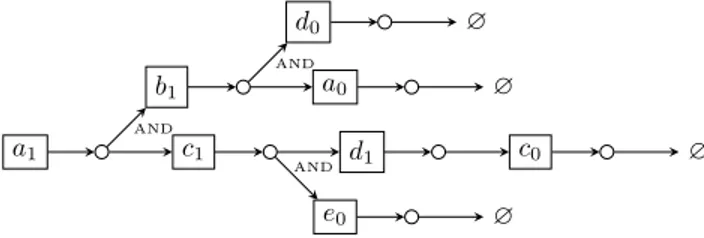
If we find a state sequence consistent with all the order constraints, we can obtain its corresponding trajectory, thus we are sure that the target state is reachable. a1 d1 e1 d0 e0 ∅ ∅ AND AND OR b1 c0 ∅ c1 b0 ∅

Figure 6: If an LCG contains such structure, the result could be inconclu-sive. However the inconclusiveness requires a1 does not possess other reachable

branches.

Still, ASPReach is not complete. A counter-example is shown in Fig. 6, when there are multiple branches of one OR gate leading to unreachability, the result can be inconclusive. There is a tricky way to deal with this issue when |ORgates| is not big: we set a limit n, if |ORgates| < n, we shift the heuristics on the assignment of OR gates to the enumeration of all possible assignments.

This “hacking” can deal with some inconclusiveness. In the benchmarks in the next section, inconclusive instances appear neither in biological examples nor in random generated tests.

We also show some algorithmic properties of ASPReach:

Theorem 3 (ASPReach termination and correctness). Let l = (Vstate, Vsolution, E)

be an LCG with initial state α and target local state ω and k > 0 be an integer. The call ASPReach(l,k) terminates.

ASP Reach(l, k)=(False, ∅) only if @t a trajectory in l from α to ω.

ASP Reach(l, k)=(True, t) only if ∃t a trajectory in l from α to ω. The proof is given in appendix B.

Theorem 4 (ASPReach complexity). Let l = (Vstate, Vsolution, E) be an LCG

with initial state α and k > 0 be an integer. Let s = |Vsolution| be the number of

target state of l. Let v = |Vstate| be the number of vertices of l. Let e = |E| be

the number of edges of l. The complexity of ASPReach(l,k) is O(v + e + v/2 × v × e × s + v2× e + v × e + k × (v × e2_{+ 2}v_{)) which is bound by O(k × 2}v_).

Proof is given in Appendix B.

4

Evaluation

In this section we evaluate our approach through various experiments. All tests were run on a Intel Core i7-3770 CPU, 3.4GHz with 8Gb of RAM computer.

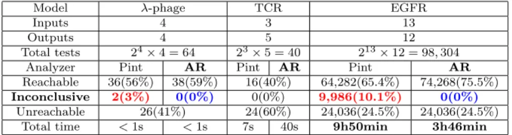
To validate our approach, we first tested a small model, λ-phage model [34] to compare with an alternative reachability analyzer Pint [27] implementing solely analysis using LCG [25, 15, 26]. In this model with 4 automata and 12 transitions (without taking consideration of the self-regulations), our result shows complete conclusiveness while Pint cannot (Fig. 7). PermReach [7] is not able either to handle some of the special cases where multiple states of one automaton appear in different branches (Fig. 8). Theses cases are solvable by ASPReach. The whole approach is implemented in Python32_{. The call of ASP}

is done by package pyasp3_.

To evaluate the scalability in in silico networks, we take T-cell Receptor model (TCR) [31] and epidermal growth factor receptor model (EGFR) [32] as examples, with the former one containing 95 automata and 206 transitions and the latter one containing 104 automata and 389 transitions respectively.

These models are originally Boolean networks. According to the approach in Appendix A, BNs are transformed into ABANs. Here, we ran the same test as in [15]. In the TCR model, we take 3 automata as input (cd4 cd28 tcrlig), varying exhaustively their initial states combinations (23), take the reachability of states of 5 automata (sre ap1 nfkb nfat sigmab) as output. Similarly we carried a bigger test on EGFR model with 13 automata as input and 12 automata as output. We first tested the performance of traditional model

2_{Code and testing data available at https://github.com/XinweiChai/LCG-in-ASP} 3_{https://pypi.python.org/pypi/pyasp}

cro1

cll0 cl1 ∅

cl0 AND

Figure 7: One LCG in λ-phage model, automaton cl appears in both branches of the AND gate. Static analyzer Pint cannot decide whether in this case cro1

is reachable or not, because it does not consider the order in the state sequence even though there exists a solution is of length 3: cll0:: cl0:: cro1corresponding

to the trajectory {cl1} → cll0:: {cll0} → cl0:: {cll0, cl0} → cro1.

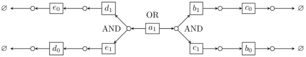
a1 b1 d0 ∅ a0 ∅ c1 d1 c0 _∅ e0 ∅ AND AND AND

Figure 8: This counterexample shows former PermReach is inconclusive if mul-tiple states of one automaton appear in the branches of one AND gate (d0

and d1 in this example). However there exists a consistent state sequence:

d1 :: b1 :: c1 :: a1 corresponding to the trajectory {c0} → d1 :: {d0, a0} → b1 ::

{d1, e0} → c1:: {b1, c1} → a1 which could be found by ASPReach.

checkers, Mole4_{and NuSMV}5_{, in which Mole turns out to be memory-out for 6}

in 12 outputs, and all memory-out for NuSMV in model EGFR. Due to the big state space, traditional model checkers are not applicable. In the TCR tests, our approach gives exactly the same result as Pint did. As for EGFR tests, ASPReach returned no inconclusive output.

As seen in Table 1, our approach can be more conclusive than Pint for ABANs. In the configuration of heuristics, we set a threshold for OR gates. If there are less than 10 OR gates after preprocessing, the computation will be shifted from heuristic to the enumeration of all combinations of OR gates. Here is the case for these three benchmarks. The experiments show the ability of ASPReach is already more conclusive than Pint in “simple” cases.

To test the global applicability of ASPReach, we ran two sets of tests on random models generated as follows: Given the number of transitions, for every transition tr, the head ahis randomly chosen from LS, the first element of the

body A1is chosen from LS1= LS \{ah, a1−h}. For i > 1, if Ai−1= bxexists, we

generate Ai with an 80% probability, choosing from LSi = LSi−1\ {bx, b1−x}.

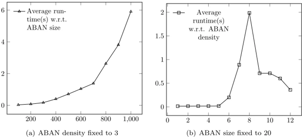
Fig. 9(a) shows the average run time of ASPReach on randomly generated

4

http://www.lsv.fr/~schwoon/tools/mole 5_{http://nusmv.fbk.eu}

Model λ-phage TCR EGFR

Inputs 4 3 13

Outputs 4 5 12

Total tests 24_{× 4 = 64 2}3_{× 5 = 40 2}13_{× 12 = 98, 304}

Analyzer Pint AR Pint AR Pint AR

Reachable 36(56%) 38(59%) 16(40%) 64,282(65.4%) 74,268(75.5%) Inconclusive 2(3%) 0(0%) 0(0%) 9,986(10.1%) 0(0%)

Unreachable 26(41%) 24(60%) 24,036(24.5%) 24,036(24.5%) Total time < 1s < 1s 7s 40s 9h50min 3h46min

Table 1: AR=ASPReach. Results of the tests on small (λ-phage) and large (TCR,EGFR) examples from biology literature. Results of model-checkers us-ing global search are memory-out so are not listed in the table. “Reachable”, “Inconclusive” and “Unreachable” give respectively the number of different re-sults of reachability. It is worth noticing that the inconclusive cases in Pint are caused by time-out [15].

ABAN. In this experiment, we fixed the number of transitions to |Σ| × 3 and each transition has a random number of heads from 1 to |Σ − 1|, with Σ the number of automata of the generated ABAN. For traditional model checkers like NuSMV and Mole, memory-out cases begin to appear when |Σ| > 50, so the runtime results are not displayable in Fig. 9(a). Also, Pint is not able to check all test sets of any |Σ|. Even though the curve of average runtime of our approach shows an exponential-like tendency, ASPReach is very fast for |Σ| < 100 (less than 0.03s) and can also perform on models with 1000 automata. Moreover, the longest runtime among the test sets is less than 20s. Because we stop the computation if one reachability check takes more than 20s and we note it as timeout. This result suggests that the heuristic approach of ASPReach has a good performance in conclusiveness in general as the testing models are generated randomly.

Another test is on the different density with the same number of automata. In Fig. 9(b), we fixed |Σ| = 20 and vary the number of the transitions per automaton (density) from 1 to 12. The runtime peak is at density 8, a possible explanation is that even the topology of the network is more complex with the growth of density, more available transitions lead to more pathways from the initial state to the target state, thus the heuristics may end with less trials.

These experimental evaluations show that ASPReach has a better scalability on reachabilty analysis than traditional exhaustive model checkers and a better performance regarding conclusiveness than existing static analyzer.

5

Conclusion

In this paper, we present the ABAN modeling framework and its model-related reachability analyzer ASPReach. Facing the two critical challenges: complexity and conclusiveness, we combine static analysis and Answer Set Programming for a good performance on both criteria. ASPReach performs normally on models

200 400 600 800 1,000 0 2 4 6 Average run-time(s) w.r.t. ABAN size

(a) ABAN density fixed to 3

0 2 4 6 8 10 12 0 0.5 1 1.5 2 Average runtime(s) w.r.t. ABAN density

(b) ABAN size fixed to 20

Figure 9: Runtime of ASPReach on random ABANs

with 1000 automata while traditional model checkers fail to compute and static analyzer Pint also fails to give conclusive results on certain instances.

We are now considering an incorporation of heuristics in the preprocessing phase, like the work of [19], to improve the performance of our approach regard-ing runtime. The development of dedicated heuristic for the orientation of the random search in ASPReach remains also a future work.

As to biological application, one path of research is the interfacing of our approach with model inference approaches. Biological models can be inferred from experimental data through machine learning techniques (e.g. [17]), but obtained models are not necessarily consistent with the a priori background knowledge about the dynamics of system. Thus it is important to check these obtained models and revise them to make them consistent with such background knowledge. In the case of reachability properties, our approach could be use as a model checker and a mean to enforce such properties in a model under construction.

References

[1] Parosh Aziz Abdulla, Per Bjesse, and Niklas E´en. Symbolic reachability analysis based on sat-solvers. In International Conference on Tools and Algorithms for the Construction and Analysis of Systems, pages 411–425. Springer, 2000.

[2] Tatsuya Akutsu, Morihiro Hayashida, Wai-Ki Ching, and Michael K Ng. Control of boolean networks: Hardness results and algorithms for tree structured networks. Journal of theoretical biology, 244(4):670–679, 2007. [3] Chitta Baral. Knowledge representation, reasoning and declarative problem

[4] Alexander Bockmayr and Arnaud Courtois. Using hybrid concurrent con-straint programming to model dynamic biological systems. In International Conference on Logic Programming, pages 85–99. Springer, 2002.

[5] Luca Bortolussi and Alberto Policriti. Modeling biological systems in stochastic concurrent constraint programming. Constraints, 13(1):66–90, 2008.

[6] Jerry R Burch, Edmund M Clarke, Kenneth L McMillan, David L Dill, and Lain-Jinn Hwang. Symbolic model checking: 1020 _{states and beyond.}

Information and computation, 98(2):142–170, 1992.

[7] Xinwei Chai, Morgan Magnin, and Olivier Roux. A Heuristic for Reachability Problem in Asynchronous Binary Automata Networks, 2018. arXiv:1804.07543v1.

[8] Allan Cheng, Javier Esparza, and Jens Palsberg. Complexity results for 1-safe nets. Theoretical Computer Science, 147(1-2):117–136, 1995. [9] Edmund Clarke, Armin Biere, Richard Raimi, and Yunshan Zhu. Bounded

model checking using satisfiability solving. Formal methods in system de-sign, 19(1):7–34, 2001.

[10] Edmund M Clarke. The birth of model checking. In 25 Years of Model Checking, pages 1–26. Springer, 2008.

[11] Edmund M Clarke and Qinsi Wang. 25 _{years of model checking. In}

In-ternational Andrei Ershov Memorial Conference on Perspectives of System Informatics, pages 26–40. Springer, 2014.

[12] Conrado Daws and Stavros Tripakis. Model checking of real-time reachabil-ity properties using abstractions. Tools and Algorithms for the Construction and Analysis of Systems, pages 313–329, 1998.

[13] Gilles Didier, Elisabeth Remy, and Claudine Chaouiya. Mapping multival-ued onto boolean dynamics. Journal of theoretical biology, 270(1):177–184, 2011.

[14] Javier Esparza. Reachability in live and safe free-choice Petri nets is NP-complete. Theoretical Computer Science, 198(1-2):211–224, 1998.

[15] Maxime Folschette, Lo¨ıc Paulev´e, Morgan Magnin, and Olivier Roux. Suffi-cient conditions for reachability in automata networks with priorities. The-oretical Computer Science, 608:66–83, 2015.

[16] Martin Gebser, Roland Kaminski, Benjamin Kaufmann, Max Ostrowski, Torsten Schaub, and Philipp Wanko. Theory solving made easy with clingo 5. In OASIcs-OpenAccess Series in Informatics, volume 52. Schloss Dagstuhl-Leibniz-Zentrum fuer Informatik, 2016.

[17] Katsumi Inoue, Tony Ribeiro, and Chiaki Sakama. Learning from inter-pretation transition. Machine Learning, 94(1):51–79, 2014.

[18] Stuart Kauffman. Homeostasis and differentiation in random genetic con-trol networks. Nature, 224:177–178, 1969.

[19] Juraj Kolˇc´ak, David ˇSafr´anek, Stefan Haar, and Lo¨ıc Paulev´e. Parameter Space Abstraction and Unfolding Semantics of Discrete Regulatory Net-works. Theoretical Computer Science, 2018. In press.

[20] Haitao Li and Yuzhen Wang. On reachability and controllability of switched boolean control networks. Automatica, 48(11):2917–2922, 2012.

[21] Haitao Li, Yuzhen Wang, and Zhenbin Liu. Stability analysis for switched boolean networks under arbitrary switching signals. IEEE Transactions on Automatic Control, 59(7):1978–1982, 2014.

[22] Vivien Marx. Biology: The big challenges of big data. Nature, 498(7453):255–260, 2013.

[23] Ernst W Mayr. An algorithm for the general Petri net reachability problem. SIAM Journal on computing, 13(3):441–460, 1984.

[24] Peter Bro Miltersen, Jaikumar Radhakrishnan, and Ingo Wegener. On converting CNF to DNF. Theoretical computer science, 347(1-2):325–335, 2005.

[25] Lo¨ıc Paulev´e. Reduction of qualitative models of biological networks for transient dynamics analysis. IEEE/ACM transactions on computational biology and bioinformatics, 2017.

[26] Lo¨ıc Paulev´e, Morgan Magnin, and Olivier Roux. Refining dynamics of gene regulatory networks in a stochastic π-calculus framework. In Transactions on computational systems biology xiii, pages 171–191. Springer, 2011. [27] Lo¨ıc Paulev´e, Morgan Magnin, and Olivier Roux. Static analysis of

bio-logical regulatory networks dynamics using abstract interpretation. Math-ematical Structures in Computer Science, 22(04):651–685, 2012.

[28] James L Peterson. Petri nets. ACM Computing Surveys (CSUR), 9(3):223– 252, 1977.

[29] Brigitte Plateau and Karim Atif. Stochastic automata network of modeling parallel systems. IEEE transactions on software engineering, 17(10):1093– 1108, 1991.

[30] Assieh Saadatpour, Istv´an Albert, and R´eka Albert. Attractor analysis of asynchronous boolean models of signal transduction networks. Journal of theoretical biology, 266(4):641–656, 2010.

[31] Julio Saez-Rodriguez, Luca Simeoni, Jonathan A Lindquist, Rebecca Hemenway, Ursula Bommhardt, Boerge Arndt, Utz-Uwe Haus, Robert Weismantel, Ernst D Gilles, Steffen Klamt, et al. A logical model pro-vides insights into T cell receptor signaling. PLoS computational biology, 3(8):e163, 2007.

[32] Regina Samaga, Julio Saez-Rodriguez, Leonidas G Alexopoulos, Peter K Sorger, and Steffen Klamt. The logic of EGFR/ErbB signaling: theoreti-cal properties and analysis of high-throughput data. PLoS computational biology, 5(8):e1000438, 2009.

[33] Robert Tarjan. Depth-first search and linear graph algorithms. SIAM journal on computing, 1(2):146–160, 1972.

[34] Denis Thieffry and Ren´e Thomas. Dynamical behaviour of biological reg-ulatory networksii. immunity control in bacteriophage lambda. Bulletin of mathematical biology, 57(2):277–297, 1995.

[35] H Steven Wiley, Stanislav Y Shvartsman, and Douglas A Lauffenburger. Computational modeling of the EGF-receptor system: a paradigm for sys-tems biology. Trends in cell biology, 13(1):43–50, 2003.

[36] Bo˙zena Wo´zna, Andrzej Zbrzezny, and Wojciech Penczek. Checking reach-ability properties for timed automata via SAT. Fundamenta Informaticae, 55(2):223–241, 2003.

A

Transformation from BNs to ABANs

Given Boolean functions vi(t + 1) = fi(Vi), with Vi the set of participating

variables among v1(t), · · · , vn(t). Boolean functions could be transformed to

equivalent CNF (conjunctive normal form) and DNF (disjunctive normal form) if the length of Boolean functions is limited to O(1) [24] which is often the case. Proposition 1 (Transformation from BN to ABAN). Given a BN GB = (V, F ),

with its functions in CNF form vi_{(t + 1) = A}

1∧ . . . Aj. . . ∧ An and DNF form

vi(t+1) = A0₁∨. . . Ak. . .∨A0m, an equivalent ABAN AB has transitions Aj→ vi1

and ¬Ak→ vi0where Aj are disjunctions and A0K are conjunctions.

Example 6. Let GB = (V, F ) a BN with V = {a, b, c, d, e}, and has only one

Boolean function, F = {f (a) = (b ∨ c) ∧ (d ∨ e)}, we have f (a) = (b ∧ d) ∨ (b ∧ e) ∨ (c ∧ d) ∨ (c ∧ e), and ¬f (a) = (¬b ∧ ¬c) ∨ (¬d ∧ ¬e). The equivalent ABAN is then constructed: 5 automata Σ = {a, b, c, d, e}, with transitions: T = {{b1, d1} →

a1, {b1, e1} → a1, {c1, d1} → a1, {c1, e1} → a1, {b0, c0} → a0, {d0, e0} → a0}.

B

Proofs

Theorem 5 (ASPReach termination and correctness). Let l = (Vstate, Vsolution, E)

The call ASPReach(l,k) terminates.

ASP Reach(l, k)=(False, ∅) only if @t a trajectory in l from α to ω. ASP Reach(l, k)=(True, t) only if ∃t a trajectory in l from α to ω.

Proof. 1: The algorithm starts by breaking all cycles of the LCG and according to Theorem 1 it terminates and does not affect the reachability of α in l.

2: Then all nodes of Vstate and (resp. solution) with no (resp. missing)

outgoing edges are removed. Such nodes cannot be part of a trajectory leading to initial state α and thus this operation does not affect the reachability of α in l. The internal for loop of this operation iterates over Vstate which is finite. To

continue looping, it requires one state deletion thus this operation will terminate atleast when Vstate becomes ∅.

Conclusion 1: ASP Reach(l, k) = False only if @t a trajectory in l from α to v ∈ Vsolution.

Conclusion 2: the call ASPReach(l,k) terminates.

Conclusion 3: After this pre-processing, pseudo reachability is checked and according to [27], it terminates and is correct. It is the only possibility for ASPReach to output False.

Conclusion 4: Stochastic search follows by randomly reducing each OR gate of l to one of its edges to form l0. This operation is run a finite time k and iterates over Vstatewhich is finite and thus it terminates. This operation does not create

new edges, i.e. E0 ⊆ E. ASP solve(l0) generates all possible trajectories of l0 leading to α. The number of possible trajectory is finite and thus ASP solve(l0) terminates.

Furthermore when ASP solve(l0) = (True, t), t is a trajectory of l proving reachability of α in l and it is the only possibility for ASPReach to output True. Conclusion 3: ASP Reach(l, k) = (True, t) only if ∃t a trajectory in l from α to v ∈ Vsolution.

Theorem 6 (ASPReach complexity). Let l = (Vstate, Vsolution, E) be an LCG

with initial state α and k > 0 be an integer. Let s = |Vsolution| be the number

of target state of l. Let v = |Vstate| be the number of vertices of l. Let e = |E|

be the number of edges of l. The complexity of ASP Reach(l, k) is O(v + s + e + (v + s)/2 × v × e × s + v2× e + v × e + k × (v × e2_{+ 2}v_{)) which is bound by}

O(k × 2v).

Proof. 1: computing SCC(l) has a complexity of O(v + s + e). In worst case |SCC(l)| = (v + s)/2 and breaking one cycle of SCC(l) is O(v × e × s), thus complexity of removing cycle is op1 = O(v + e + s + (v + s)/2 × v × e × s)

2: To remove useless nodes ASPReach iterates over all states and checking if one state has no successor in l requires to iterates over all edges. In worst case all states will be removed one by one and thus the complexity of this operation is op2 = O(v × (v + s) × e).

3: Computing pseudo reachability over l which have no loop correspond to perform a depth first search on all branch of a tree and thus bound to op3 = O((v + s) × e).

4: the stochastic search iterates atmost k times. Treating each OR gate to form l0 have a cost of O(v × e × e) ASP solve(l0) generates trajectories that can prove reachability of α in l0. Each trajectory is a sequence where each element of |Vstate| appears exactly once. It correspond to the number of total order

of |Vstate| which is 2v. Thus ASP solve(l0) is bound by O(2v) and the whole

stochastic search by op4 = O(k × (v × e2_{+ 2}v_)).

Conclusion 1: The complexity of ASP Reach(l, k) is O(op1 + op2 + op3 + op4) = O(v + e + s + (v + s)/2 × v × e × s + v × (v + s) × e + v × e + k × (v × e2_{+ 2}v_)).

Conclusion 2: The complexity of ASP Reach(l, k) is bounded by O(k × 2v₎

C

Pseudo Code of Pseudo-reachability

Algorithm 3 Pseudo-reachability reach0

Input: an LCG l = (Vstate, Vsolution, E), an initial state α, a target state ω

Output: a Boolean reach0 procedure pseudoReach(s)

// If ω is in initial state, it is already reached

if ω ∈ α then return True

// The reachability of s depends on its successor solution nodes

if 6 ∃(s, sol) ∈ E then return False for each (s, sol) ∈ E do

if fireable(sol) then return True return False

procedure fireable(sol) for each (sol, s0) ∈ E do

if pseudoReach(s0) then return False return True