A bootstrap method for comparing correlated kappa coefficients

Vol. 00, No. 00, Month 200x, 1–15

A bootstrap method for comparing correlated kappa

1

coefficients

2

S. Vanbelle† ∗ _{and A. Albert}†

3

†_{Medical Informatics and Biostatistics, School of Public Health, University of Li`ege,}

4

CHU Sart Tilman, 4000 Li`ege, Belgium

5

(Received 00 Month 200x; In final form 00 Month 200x) 6

Cohen’s kappa coefficient is traditionally used to quantify the degree of agreement between two raters 7

on a nominal scale. Correlated kappas occur in many settings (e.g. repeated agreement by raters on 8

the same individuals, concordance between diagnostic tests and a gold standard) and often need to 9

be compared. While different techniques are now available to model correlated κ coefficients, they 10

are generally not easy to implement in practice. The present paper describes a simple alternative 11

method based on the bootstrap for comparing correlated kappa coefficients. The method is illustrated 12

by examples and its type I error studied using simulations. The method is also compared to the 13

generalized estimating equations of second order and the weighted least-squares methods. 14

Keywords: Cohen’s kappa, comparison, bootstrap 15

16

Medical Informatics and Biostatistics, School of Public Health, University of Li`ege, CHU Sart Tilman, 4000 Li`ege, Belgium, sophie.vanbelle@ulg.ac.be

1 Introduction

17

The kappa (κ) coefficient proposed by Cohen [1] in 1960 is widely used to as-18

sess the degree of agreement between two raters on a binary or nominal scale. 19

It corrects the observed percentage of agreements between the raters for the ef-20

fect of chance. Thus, a value of 0 implies no agreement beyond chance, whereas 21

a value of 1 corresponds to a perfect agreement between the two raters. Corre-22

lated kappas can occur in many ways. For example, two raters may assess the 23

same individuals at various occasions or in different experimental conditions 24

and it may be of interest to test for homogeneity of the kappas. Alternatively, 25

each member of a group of raters may be compared to an expert in assessing 26

the same items on a nominal scale. Are there differences between the indi-27

vidual kappas obtained? The same problem arises when comparing several 28

diagnostic tests on a binary scale (negative/positive) with respect to a gold 29

standard. Fleiss [2] developed a method based on the chi-square decomposition 30

for comparing two or more κ coefficients but only applicable to independent 31

samples. McKenzie et al. [3] proposed an approach based on resampling for 32

the comparison of two correlated κ coefficients. With the advent of generalized 33

linear mixed models, it is now possible to model the coefficient κ as a function 34

of covariates. Williamson et al. [4] used the generalized estimating equations 35

of second order (GEE2) to model correlated kappas. Lipsitz et al. [5] proposed 36

an empirical method to model independent κ coefficients. Finally, Barnhart 37

and Williamson [6] used the weighted least-squares approach (WLS) to model 38

correlated κ coefficients with respect to categorical covariates. All modeling 39

techniques represent a considerable progress but they require adequate model 40

specifications and expert programming skills. Currently, no simple method can 41

be found in the literature for comparing several correlated κ coefficients. The 42

present paper describes a practical and feasible alternative to the modeling 43

techniques by expanding the resampling method based on bootstrap proposed 44

by McKenzie et al. [3]. The original method is exposed in Section 2 and the 45

extension detailed in Section 3. Simulations of the type I error are given in 46

Section 4 for different levels of the kappa coefficient and different sample sizes. 47

Results are compared to those obtained by the GEE2 and the WLS methods. 48

The bootstrap, GEE2 and WLS methods were applied to two examples in 49

Section 5. Finally, results are discussed in Section 6. 50

2 Bootstrapping two correlated kappas

51

Suppose that two raters classify n subjects on a binary or nominal scale at 52

two different occasions or in two different experimental settings. Let ˆκ1and ˆκ2 53

be the kappa coefficients obtained. Since the two agreements are assessed on 54

the same subjects, ˆκ1 and ˆκ2 are correlated. Are they statistically different? 55

Let H0 : κ1 = κ2, the null hypothesis to be tested. The bootstrap method 56

consists in drawing q samples (1000 is generally sufficient [3]) of size n with 57

replacement. For each generated sample, the κ coefficient between the 2 raters 58

is estimated in the two settings and their difference bκd= bκ2− bκ1 calculated. 59

McKenzie et al. [3] suggested to determine the bootstrap two-sided (1 − α)-60

confidence interval for the ˆκddifferences, whence rejecting the null hypothesis 61

if the confidence interval did not include 0. This approach is equivalent to 62

using a Student’s t-test and to reject H0 at the α-significance level if 63 |tobs| = ¯ ¯ ¯ ¯ κd SE(κd) ¯ ¯ ¯ ¯ ≥ Qt(1 − α/2; q − 1) (1)

where κd and SE(κd) are respectively the mean and standard deviation of 64

the q bootstrapped kappa differences and Qt(1 − α/2; q − 1) is the upper α/2-65

percentile of the Student’s t distribution on q−1 degrees of freedom. Otherwise, 66

H0 is not rejected. 67

3 Extension to several correlated kappas

68

Suppose we want to compare G ≥ 2 correlated kappa coefficients (κ1, · · · , κG) 69

i.e., to test the null hypothesis H0 : κ1 = · · · = κG against the alternative 70

hypothesis H1 : ∃k 6= l ∈ {1, · · · , G} : κk 6= κl. As before, the bootstrap 71

method will consist in drawing q samples of size n with replacement from 72

the original data. Then, for each bootstrapped sample (j = 1, · · · , q), let 73

b

κ_{j = (bκ1(j), · · · , bκG(j))}′ _{be the vector of the G kappa coefficients obtained. The} 74

null and alternative hypotheses can be rewritten in matrix form as follows: 75

H0 : Cκ = 0 versus H1 : Cκ 6= 0, where κ = (κ1, · · · , κG)′ and C the 76 (G − 1) × G patterned matrix 77             1 −1 0 · · · 0 1 0 −1 · · · 0 · · · · 1 0 0 · · · −1            

Then, the test statistic is 78

T2 = (Cκ)′_(CSC′₎−1_{Cκ (2)}

distributed as Hotelling’s T2, where κ and S are respectively the sample mean 79

vector and covariance matrix of the q bootstrapped vectors ˆκ_{. The null} hy-80

pothesis will be rejected at the α-level if 81

T2 ≥ (q − 1)(G − 1)

(q − G + 1) QF(1 − α; G − 1, q − G + 1) (3) where QF(1−α; G−1, q −G+1) is the upper α-percentile of the F distribution 82

on G − 1 and q − G + 1 degrees of freedom. Otherwise, H0 will not be rejected. 83

Note that, since “q − G + 1” will be large in general, the left-hand side of 84

equation 3 can be approximated by Qχ2(1 − α; G − 1), the (1 − α)th percentile

85

of the chi-square distribution on G − 1 degrees of freedom. If cg denotes the g-86

th row of matrix C, simultaneous confidence intervals for individual contrasts 87 c′ gκ(g = 1, · · · , G − 1) given by 88 c′ gκ± s (q − 1)(G − 1) (q − G + 1) QF(1 − α; G − 1, q − G + 1) q c′ gScg (4)

can be used for multiple comparison purposes. 89

4 Simulations

90

The method described in Section 3 was applied to simulated data sets in order 91

to study the behavior of the type I error (α) of the homogeneity test for G = 3. 92

Each simulation consisted in applying the bootstrap method to 3000 data sets 93

generated under the null hypothesis H0 : κ1 = κ2 = κ3 and to determine 94

the number of times H0 was rejected. The simulated data set was based on 95

4 binary random variables X, Y , Z and V . The agreement between X and 96

Y (κXY), X and Z (κXZ) and X and V (κXV) were compared using the 97

bootstrap method with q = 2000 iterations. Simulations were repeated for 3 98

sample sizes (50, 75 and 100) and 5 levels of agreement (κ=0, 0.2, 0.4, 0.6 99

and 0.8). To obtain a given level of agreement (κ), 2 vectors of size n from 100

binary random variables (U and W ) were generated. Then, a vector of size n 101

with uniform random numbers between 0 and 1 was generated. Each time the 102

random uniform number was less than or equal to the given level of agreement 103

(κ), the value of W was changed into the value of U , otherwise it remained 104

unchanged. The kappa coefficient was derived from the 2 × 2 table obtained 105

by cross-classifying the vectors U and W . The codes for the simulations were 106

written in R language using uniform random number generator with seed 107

equal to 2. The method of generalized estimating equations of second order 108

(GEE2) [4] and the weighted least square approach (WLS) [6] were also applied 109

to the 3000 simulated data sets. Results are summarized in Table 1. It is seen 110

that type I error rates obtained with the bootstrap method are slightly but 111

systematically higher than the expected 5% nominal level. While the GEE2 112

approach appears to be optimal, the bootstrap was better than the WLS, at 113

least for elevated κ values. However, the bootstrap method may be preferred 114

to the GEE2 approach because of the ease of implementation in all settings as 115

compared to the GEE2 method, which requires the writing of a lengthy and 116

specific program for each particular problem. 117

5 Examples

118

5.1 Deep venous thrombosis

119

A study was conducted on 107 patients in the medical imaging department of 120

the university hospital (unpublished data) to compare deep venous thrombosis 121

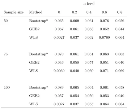
Table 1. Type I error for the comparison of G = 3 correlated kappa coefficients, according to κ level and sample size (figures are based on 3000 simulations each)

κ level

Sample size Method 0 0.2 0.4 0.6 0.8 50 Bootstrapa _{0.065 0.069 0.061 0.076 0.056} GEE2 0.067 0.061 0.063 0.052 0.044 WLS 0.0027 0.037 0.062 0.0769 0.064 75 Bootstrapa _{0.070 0.061 0.061 0.063 0.063} GEE2 0.046 0.058 0.057 0.051 0.040 WLS 0.0030 0.040 0.060 0.071 0.069 100 Bootstrapa _{0.089 0.065 0.064 0.061 0.058} GEE2 0.057 0.054 0.050 0.053 0.040 WLS 0.0027 0.037 0.055 0.064 0.064 a _{q = 2000}

(DVT) detection using a multidetector-row computed tomography (MDCT) 122

and ultrasound (US). The study also looked at the benefit of using spiral 123

(more images and possibility of multiplanar reconstructions) with respect 124

to sequential technique (less slices, less irradiation). Images were acquired 125

in the spiral model (ankle to inferior vena cava) and reconstructed in 5 mm 126

thickness slices every 5 mm, 20 mm and 50 mm. Two radiologists (one junior 127

and one senior) assessed for each patient and each experimental setting (5/5, 128

5/20 and 5/50 slices) the presence of DVT. The aim of the study was to 129

compare agreement of the different MDCT slices with the US method. Only 130

data of the senior radiologist will be presented here (see Table 2). 131

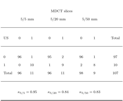
Table 2. Cross-classification of DVT detection (0=absence, 1=presence) using different MDCT slices (5/5, 5/20 and 5/50 mm) and US in 107 patients by a senior radiologist (unpublished data)

MDCT slices 5/5 mm 5/20 mm 5/50 mm US 0 1 0 1 0 1 Total 0 96 1 95 2 96 1 97 1 0 10 1 9 2 8 10 Total 96 11 96 11 98 9 107 κ5/5= 0.95 κ5/20= 0.84 κ5/50= 0.83 132

The observed kappa coefficients (± SE) were 0.95 ± 0.053, 0.84 ± 0.089 and 133

0.83 ± 0.098 for 5/5, 5/20 and 5/50 mm slices, respectively. The bootstrap 134

approach with 2000 iterations led to a Hotelling’s T2 value of 1.46 (p=0.48) 135

indicating no evidence of a difference between the κ coefficients at the 5% sig-136

nificance level. The bootstrap estimates of bias were 0.003, 0.008 and 0.009 for 137

the 5/5, 5/20 and 5/50 mm slices, respectively. According to the rule described 138

in Efron [9], the bias can be ignored. The differences between the κ generated 139

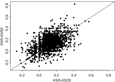
by the 2000 iterations of the bootstrap are represented in Figure 1 with the 140

95% confidence ellipse for the difference vector (κ5/5− κ5/20, κ5/5 − κ5/50). 141

K5/5-K5/20 -0.2 0.0 0.2 0.4 0.6 0.8 -0.2 0.0 0.2 0.4 0.6 0.8 K5/5-K5/50 + +

Figure 1. Kappa differences (κ5/5− κ5/50versus κ5/5− κ5/20) generated by the bootstrap (q=2000) with 95% confidence interval.

It is seen that the origin (0, 0) is well inside the confidence region, as expected. 142

143

5.2 Diagnosis of depression

144

McKenzie et al. [3] compared for illustrative purposes the agreement between 145

two different screening tests (Beck Depression Inventory (BDI) and General 146

Health Questionnaire (GHQ)) and the diagnosis of depression including 147

DSM-III-R Major depression, dysthymia, adjustment disorder with depressed 148

mood and depression not otherwise specified (NOS). The study consisted in 149

determining presence or absence of depression in 50 patients. Data are sum-150

marized in Table 3. McKenzie et al. found that the 95% bootstrap confidence 151

Table 3. Depression (0=absence, 1=presence) assessed in 50 patients ac-cording to two screening tests (BDI and GHQ) and to a medical diagnosis

BDI GHQ

Depression diagnosis 0 1 0 1 Total

0 35 2 34 3 37

1 6 7 2 11 13

Total 41 9 36 14 50

κBDI= 0.54 κGHQ= 0.75

interval based on the percentiles for the difference between the two kappas 152

did include 0. The kappa coefficients were 0.54 ± 0.14 between diagnosis of 153

depression and BDI and 0.75 ± 0.11 between diagnosis of depression and 154

GHQ, respectively. The bootstrap method described in Section 3 resulted 155

in a T2 value of 2.19 (p=0.14) confirming the findings of McKenzie [3]. The 156

bootstrap estimates of bias were 0.008 and 0.009 for BDI and GHQ methods, 157

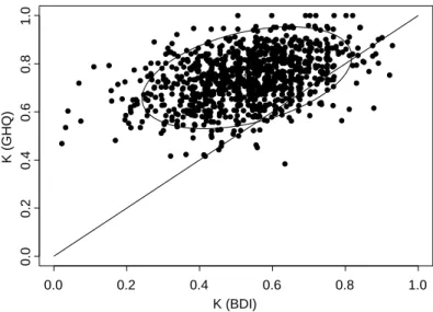
respectively, and could be ignored. Figure 2 displays the kappa values for 158

BDI and GHQ generated by the bootstrap method (q = 1000) with the 159

corresponding 95% confidence interval. 160

K (BDI) 0.0 0.2 0.4 0.6 0.8 1.0 0.0 0.2 0.4 0.6 0.8 1.0 K (GHQ) +

Figure 2. Kappa values of BDI and GHQ for the diagnosis of depression generated by the bootstrap (q = 1000) with 95% confidence interval

5.3 Application of WLS and GEE2 approaches

162

The weighted least squares method developed by Barnhart and Williamson [6] 163

and the GEE2 approach of Williamson et al. [4] were also applied to both 164

datasets. As seen in Table 4, these approaches led to the same conclusions as 165

the bootstrap procedure for both examples. 166

6 Discussion

167

The comparison of two or more correlated kappa coefficients is a frequently 168

encountered problem in real life practice and there is no simple handy test to 169

solve it. The bootstrap method described in this work provides an estimate of 170

Table 4. Comparison of the bootstrap, the GEE2 and the weighted least squares (WLS) ap-proaches applied to the radiology data (unpublished) and the depression data of McKenzie [3]

Bootstrap GEE2 WLS

κ SE p-value κ SE p-value κ SE p-value DVT radiology data 5/5 mm 0.95 0.056 0.48 0.95 0.048 0.56 0.95 0.053 0.46 5/20 mm 0.84 0.096 0.84 0.060 0.84 0.089 5/50 mm 0.83 0.108 0.83 0.063 0.83 0.098 Depression data BDI 0.54 0.144 0.14 0.54 0.115 0.13 0.54 0.141 0.13 GHQ 0.75 0.114 0.75 0.128 0.75 0.107

the mean and the variance-covariance matrix of correlated kappa coefficients 171

and hence a way to test their homogeneity by means of the Hotelling’s T2_. 172

This extension of the resampling method proposed by McKenzie et al. [3] 173

provides an alternative to the existing advanced techniques of modeling κ 174

coefficients. Furthermore, it can be used for the comparison of other correlated 175

agreement or association indexes, like the intraclass kappa coefficient [7] and 176

the weighted kappa coefficient [8] for example. The weighted least squares 177

method developed by Barnhart and Williamson [6] and the GEE2 approach of 178

Williamson et al. [4] led to the same conclusions as the bootstrap procedure 179

for both examples, although estimates of the κ coefficients obtained with the 180

bootstrap method were slightly biased. However, Efron [9] suggested that if the 181

estimate of the bias ( ˆbias) is small compared to the estimate of the standard 182

error ( ˆSE), i.e. bias/ ˆˆ SE ≤ 0.25, the bias can be ignored. Otherwise, it may 183

be an indication that ˆκ is not an appropriate estimate of the parameter κ. 184

The bootstrap approach also yields slightly higher standard errors than the 185

WLS and the GEE2 methods, as it was expected from the results of the 186

simulations. Indeed, the type I errors obtained with the bootstrap method were 187

more liberal than those with the GEE2 method, in particular if the sample 188

size (n) was small with respect to the number (G) of kappas to be compared. 189

This finding confirms the remark made by McKenzie [3] et al. Nevertheless, 190

the type I error obtained by the bootstrap remains acceptable although it is 191

recommended to use more than 1000 bootstrap iterations when the number of 192

κ coefficients to be compared is greater than 2. The method outlined in Section 193

3 can be easily implemented in many statistical packages and programming 194

languages since the method merely requires the generation of random uniform 195

numbers and simple matrix calculations. By contrast, modeling techniques 196

require specific programming for each problem encountered in practice. Their 197

use is nevertheless highly recommended when it comes to account for many 198

covariates. A function for the bootstrap method was developed in R language 199

and is available on request from the first author. 200

The authors are grateful to Dr B. Ghaye, senior radiologist at the university 201

hospital, for providing the medical imaging data. 202

References

203

[1] Cohen J., 1960, A coefficient of agreement for nominal scales., Educational and Psychological 204

Measurement, 20, 37–46. 205

[2] Fleiss J.L. , 1981, Statistical methods for rates and proportions, (2nd edn) (Wiley, New York). 206

[3] McKenzie D.P. et al., 1996, Comparing correlated kappas by resampling: is one level of agreement 207

significantly different from another? Journal of psychiatric research, 30, 483–492. 208

[4] Williamson J.M. et al., 2000, Modeling kappa for measuring dependent categorical agreement 209

data, Biostatistics, 1, 191–202. 210

[5] Lipsitz S.R. et al., 2001, A simple method for estimating a regression model for κ between a pair 211

of raters, Journal of the Royal Statistical Society A, 164, 449–465. 212

[6] Barnhart H.X. and Williamson J.M., 2002, Weighted least-squares approach for comparing cor-213

related kappa, Biometrics, 58, 1012–1019 214

[7] Kraemer H.C., 1979, Ramification of a population model for κ as a coefficient of reliability, 215

Psychometrika, 44, 461–472 216

[8] Cohen J., 1968, Weighted kappa: nominal scale agreement with provision for scaled disagreement 217

or partial credit, Psychological bulletin, 70, 213–220 218

[9] Efron B. and Tibshirani R.J., 1993, An introduction to the bootstrap, (Chapman and Hall, New 219

York). 220