• Aucun résultat trouvé

An educational simulation tool for power system control and stability

N/A
N/A
Protected

Academic year: 2021

Partager "An educational simulation tool for power system control and stability"

Copied!
9
0
0

Texte intégral

(1)

Abstract—This paper presents a Simulink-based educational tool developed for the purpose of illustrating power system con-trol and stability notions as well as introducing students to realis-tic, though tractable in size, design problems. Relevant courses are taught to last-year undergraduate as well as graduate stu-dents at the University of Liège, Belgium and the National Tech-nical University of Athens, Greece. After a brief description of the corresponding curricula, the paper describes the simulation tool and gives examples of problems and assignments given to the stu-dents.

Index Terms—Power System Control, Power System Stability, Computer Simulation, Matlab, Simulink.

I. INTRODUCTION

HIS paper presents an educational tool for teaching power system control and stability. The corresponding software has been developed within the environment of Matlab and Simulink, which are well-known tools in the power engineer-ing area, as they have been used for load flow calculations, small-signal analysis of electromechanical oscillations and transient stability analysis [1-5], as well as the simulation of electromagnetic transients [6]. The paper also describes the application of the developed tool for preparing design projects and exercises given to last-year undergraduate, as well as graduate, students of the National Technical University of Athens, Greece (NTUA) and the University of Liège, Belgium (ULg).

The idea of using Simulink to develop an educational pack-age for the analysis of Power System Dynamics first arose in 1997 at ULg and matured progressively, in particular within the context of a collaboration with the University of Bologna [7]. On the lines of this original idea various modules simulat-ing power system components have been developed at ULg, as well as in the Electrical Energy Systems Lab of NTUA. These include generic models of traditional components (synchro-nous generator, AVR, governor, voltage-dependent loads, in-duction motor, SVC, etc.), as well as specific models for FACTS devices, steam and hydro power plants, wind parks

C. D. Vournas is professor in the School of Electrical  Computer Engi-neering in NTUA, Greece (e-mail: vournas@power.ece.ntua.gr).

E. G. Potamianakis is graduate student at the same school (e-mail: manpot@power.ece.ntua.gr)

C. Moors is research engineer at the Dept. of Electrical Engineering and Computer Science (Institut Montefiore) of the University of Liege, Belgium.

T. Van Cutsem is research director, FNRS (Belgian national fund for sci-entific research) and adjunct professor at the same department (e-mail: t.vancutsem@ulg.ac.be).

with induction generators, etc. More recently, the software has been extended to simulate autonomous (e.g. island) systems, in which the frequency dependence of network and component parameters is explicitly modeled [14].

Section II briefly presents the NTUA and ULg Electrical Engineering curricula. The Simulink Educational Tool is de-scribed in Section III, both in general terms and through an example. Section IV presents a sample of design projects and exercises given to both ULg and NTUA students. The paper ends with conclusions commenting upon student response.

II. CURRICULA STRUCTURE

The undergraduate curricula of NTUA and ULg follow the continental European tradition of 5-year programs leading directly to an Engineering Diploma equivalent to an MSc gree. The corresponding structure for each University is de-scribed below.

A. NTUA Curriculum

The 5-year NTUA curriculum for Electrical and Computer Engineers has a common core lasting for 5 Semesters, fol-lowed by a series of course “strings” that allows a wide but structured selection among a variety of Electrical and Comput-er EngineComput-ering fields. Out of a total of 10 such strings, such as “Electric Energy Systems”, “High Voltage, Machines and Power Electronics”, “Telecommunications”, “Computer Net-works”, “Electronics and Circuits”, “Computer Hardware”, “Computer Software”, “Systems, Control, and Robotics”, etc. the students have to select two full strings and two comple-mentary (or half) strings. A full string consists of 4 required and 3 elective courses, whereas a complementary string is made up of 2 required and 2 elective courses. Thus each stu-dent can realize a particular profile that combines a wide spec-trum within the Electrical and Computer Engineering disci-pline with an in-depth knowledge in the selected fields. The last (10th) Semester is devoted to the preparation of a Diploma

Thesis, which is similar to an MSc dissertation.

One of the 9th Semester elective courses of the “Electric

Energy Systems” string is on “Power System Control and Sta-bility”. The course covers modeling aspects of steam and hy-dro power plants, frequency control, voltage control, small signal stability including stabilizer design, and finally transient stability. The educational tool presented in this paper is used within this course as will be explained in Section IV.

An Educational Simulation Tool for

Power System Control and Stability

C. D. Vournas, E. G. Potamianakis, C. Moors and T. Van Cutsem

(2)

B. ULg Curriculum

The 5-year engineering curriculum at the University of Liege is organized as follows.

The first two years are common to almost all engineering orientations and cover basic disciplines such as Mathematics, Physics, Chemistry, Computer Programming, etc. The choice between Electrical, Mechanical, Civil, Chemical, Computer, etc. engineering has to be made at the beginning of the 3rd year. In the case of Electrical Engineering, a further choice between "electronics" and "power engineering" can be made at the beginning of the 4th year. Attention is paid, however, to keeping the degree multi-disciplinary; in this respect, the two orientations still have many courses in common. Part of the last year is devoted to an important personal project, to be de-fended. This brings the diploma to the Master degree.

Elective courses can be taken during the last two years. The educational tool presented in this paper is used in one of them, named "Electric power systems: dynamic aspects". This course is attended by last-year undergraduate students, as well as by graduate students applying for the D.E.A. ("Diplome d'Etudes Approfondies") in Electric Energy Systems, or the Ph.D. de-gree. It is also attended by students from other European coun-tries, within the context of the ERASMUS exchange program.

Following the adhesion of the Belgian universities to the Bologna treaty (aimed at making curricula more uniform throughout European Union), the engineering curriculum is being re-designed according to the 3-5 scheme. As far as Elec-trical Engineering is concerned, the first three years will lead to the diploma of Bachelor in Engineering and the last two to the Master in Electrical Engineering.

III. SIMULINK EDUCATIONAL TOOL A. Motivation

With the increased power transfers taking place in the new electricity markets, dynamic performance and stability is be-coming a major concern in the design and operation of many power systems. Beside steady-state security aspects (thermal overloads, voltage drops), it is therefore of particular interest to have dynamics and stability aspects [8] covered in a power system engineering curriculum.

Detailed and efficient industry software is available for dy-namic analysis. Professional software, however, is not well suited for classroom purposes, as the embedded models may lack transparency, their modification may be difficult, and it takes time to master complex software. Also, students may not have an easy access to the tool. Matlab, on the other hand, is already widely used in engineering curricula and well known by students.

This section describes how Simulink, the well-known envi-ronment for dynamic system simulation, has been used for the development of a versatile, yet clear, library of power system components. The developed tool is used to illustrate power system dynamic behavior to students, introduce them to basic notions of stability and initiate them into design projects using suitable analysis methods.

This library of Simulink models for time-domain simulation is complemented by Matlab (m-file based) analysis tools, e.g. for small-signal stability analysis.

B. Main modeling assumptions

The model of concern here relies on the well-known quasi-sinusoidal (or phasor) approximation of power system dynam-ics, and takes on the differential-algebraic form:

x' = f ( x, V, zk) (1)

0 = I ( x, V, zk ) – Y V (2)

zk+1 = h (zk, V, zk) (3) where:

 (1) stems from the short-term dynamics of synchronous generators, AVRs, governors, induction machines, SVCs, etc. x is the corresponding state vector;

 (2) are the network equations, where I (resp. V) is the vector of complex currents injected into network (resp. bus voltages) and Y is the network complex admittance matrix. All I and V components refer to a set of axes ro-tating at nominal angular frequency (synchronous frame);  (3) stems from the discrete-type dynamics of switching

devices such as OverExcitation Limiters (OELs) and Load Tap Changers (LTCs). zkis the corresponding vector of discrete variables.

C. Main features of the tool

When developing this educational tool, attention has been paid to the following aspects:

 modularity and expandability: models are structured ac-cording to a clear hierarchy. For instance, a power system is primarily seen as a collection of power plant, load, compensation, etc. blocks, interconnected through the network. In turn, each power plant is a subsystem made up of a synchronous generator, an excitation-AVR and a tur-bine-governor block. Various models for these blocks can be graphically interchanged;

 simplicity of use: each dynamic block has a user-friendly interface for data acquisition and automatically initializes its internal state variables from a data structure describing the initial operating point. This structure, as well as the network Y matrix, are produced automatically by an ex-ternal program;

 transparency: the graphic representation closely matches the theoretical models and the interface variables between blocks are meaningful. Programming tricks and shortcuts have been avoided to the greatest extent, even at the cost of computational efficiency.

Thanks to its modularity the model library can be used to il-lustrate a wide range of phenomena, such as:

 angle stability: small signal (damping of electromechani-cal modes) and transient (response to short-circuits)  frequency control and stability: load frequency control,

hydro-turbine effects, islanded operation after network split

 voltage stability: short-term (induction machines) and long-term (LTC, OEL, load restoration).

(3)

Matlab environment, using m-files include:

 identification of Park inductance matrices from Xd, X’d, X’’d, etc. reactances and T’do, T’’do , etc. time constants  post-processing of outputs

 modal analysis and computation of participation factors to analyze modes of interest

 determination of transfer functions and computation of residues for feedback control design, etc.

D. Example

The following example is aimed at illustrating some salient features of the Simulink implementation. The simple 3-bus system of Fig. 1 (used in ULg lectures on voltage stability) is considered; it is very close to one described in [9].

network (equiv.) 380 kV G 2 1 3 LTC controlled load

Fig. 1. One-line diagram of the example system

The top-level view of the Simulink model is given in Fig. 2, where two tags such as V1 and V1 indicate a connection, hidden to preserve legibility. Note how each component is represented by a separate block and all are connected through the network block.

Fig. 2. Simulink top-level view of the system

Each component, i.e. the Thévenin equivalent, the thermal plant and the load block receives its terminal voltage as input and produces the injected current as output. Conversely, the network block has the currents as inputs and the bus voltages as outputs.

An internal view of the thermal power plant subsystem is given in Fig. 3, showing respectively the synchronous genera-tor, the AVR (equipped with an OEL) and the steam turbine. Expectedly, the interface variables are the mechanical torque (Tm), the rotor speed (omega), the field voltage (vf) and the field current (if).

Fig. 3. Internal view of the thermal power plant subsystem Finally, an internal view of the synchronous generator block is given in Fig. 4. The machine is represented by a Park model with 4 rotor windings, in the reciprocal per unit system. The state variables are the flux linkages (psir) together with the rotor angle (delta) and speed (omega).

Fig. 4. Internal view of the synchronous generator block

The handling of the network equations (2) is a key point of any time simulation method. Two variants are available.

The first, and most “transparent” approach is shown in Fig. 5, giving an internal view of the “network” sub-system of Fig. 2. The algebraic constraints (2) are explicitly enforced by the upper-right block. The output of this block is the vector of bus voltages while its input is the right-hand side of (2). The figure also shows the “switch” that permits the admittance ma-trix to change during the simulation, in order to simulate faults and equipment tripping. In the case of Fig. 5 the system goes through two successive configurations.

The presence of nonlinear algebraic constraints, however, is known to slow down the execution of Simulink. This can be overcome if the currents I linearly depend on the voltages V, i.e.

(4)

Fig. 5. Internal view of the network sub-system

I ( x, V, zk ) = A(x) V +  (x, zk ) (4) where  does not explicitly depend on V. Indeed, in this case, Eq. (2) can be rewritten as

V = [Y

– A(x) ]

-1  (x, zk) (5) which can be substituted in (1) and (3), thereby eliminating the algebraic constraints. The relationship (4) holds true when loads are linear [10], or alternatively, nonlinear load models are replaced by a multiplicative restorative model with short-term impedance behaviour [9] (p. 128). The generality of the model is thus preserved while the efficiency of the solver is greatly enhanced.

This has led to develop a second variant of the tool, in which each power system component passes to the network block the (x, zk) component of its current as well as its con-tribution to the A matrix.

E. Some implementation aspects

Simulink offers the possibility to “mask” a sub-system, which allows to provide it with a user interface for data acqui-sition, as well as Matlab initialization commands.

As an example, Fig. 6 shows the interface relative to the synchronous generator of Fig. 4. Such an interface is used to assign values to the parameters of the corresponding masked sub-system. By so doing, no dynamic data are read from a file; rather, they are defined and readily available for inspection where they are used.

The initialization commands are used to determine the ini-tial values of the sub-system state variables from the output of the initial load flow. To this purpose, the initial operating point is stored in a Matlab “structure array” whose fields are the bus voltage magnitudes, phase angles, active and reactive power injections, respectively. A fragment of such a structure is shown in Fig. 7. The latter is passed to each sub-system through its data acquisition interface. In Fig. 6, for instance, the circled entry of the interface is the name of this structure (opt).

In the variant with explicit handling of the nonlinear alge-braic constraint (see Fig. 5), the admittance matrices and the initial operating point structure are directly taken from the Matlab workspace.

Fig. 6. Data acquisition interface of the synchronous generator block

opt(1).name = 'EQUIV' ; opt(1).magv = 1.10000 ; opt(1).phav = 0.00000 ; opt(1).injp = 1050.00 ; opt(1).injq = 538.683 ; opt(2).name = 'GENER' ; opt(2).magv = 0.977700 ; opt(2).phav = -0.190233 ; opt(2).injp = 450.000 ; opt(2).injq = 115.472 ;

Fig. 7. Example of structure defining the initial operating point (fragment) In the variant with linear constraints eliminated using (4), the block of Fig. 5 is replaced by an “S-function”, i.e. (5) is implemented through Matlab code in an M-file. By way of example, the code relative to the system of Fig. 1 is shown in Fig. 8.

It is noteworthy that all Matlab codes used to initialize the system (see Fig. 7) or define the pre-disturbance admittance matrix (see Fig. 8) are automatically produced by an external program, making it easy to change operating point or network data.

IV. SAMPLE PROJECTS AND EXERCISES

The developed tool is used in both Universities for various educational activities:

 classroom demonstration to illustrate concepts and help in the analysis

 simple exercises for which the students use the tool to answer specific questions and explain dynamic responses

(5)

function [sys,x0,str,ts] = network(t,x,u,flag) switch flag,

case 0,

sizes = simsizes; sizes.NumContStates = 0; sizes.NumDiscStates= 0; sizes.NumOutputs = 6 ; sizes.NumInputs = 10 ; sizes.DirFeedthrough = 1; sizes.NumSampleTimes = 1; sys = simsizes(sizes); x0 = []; str = []; ts = [-1 0]; case 3, Y=zeros( 3) ; % Contributions of branches to Y Y( 1, 3)=Y( 1, 3)+ 0.000 + 18.095238 *j ; Y( 3, 1)=Y( 3, 1)+ 0.000 + 18.095238 *j ; Y( 1, 1)=Y( 1, 1)+ 0.000 + -18.095238 *j ; Y( 3, 3)=Y( 3, 3)+ 0.000 + -18.095238 *j ; Y( 1, 3)=Y( 1, 3)+ 0.000 + 18.095238 *j ; Y( 3, 1)=Y( 3, 1)+ 0.000 + 18.095238 *j ; Y( 1, 1)=Y( 1, 1)+ 0.000 + -18.095238 *j ; Y( 3, 3)=Y( 3, 3)+ 0.000 + -18.095238 *j ; Y( 2, 3)=Y( 2, 3)+ 0.000 + 60.096153 *j ; Y( 3, 2)=Y( 3, 2)+ 0.000 + 60.096153 *j ; Y( 2, 2)=Y( 2, 2)+ 0.000 + -62.499996 *j ; Y( 3, 3)=Y( 3, 3)+ 0.000 + -57.784763 *j ; % Contributions of shunts to Y % Contributions of machines to Y Y( 1, 1)=Y( 1, 1)+ u( 3,1)+ j* u( 4,1) ; Y( 2, 2)=Y( 2, 2)+ u( 7,1)+ j* u( 8,1) ; % Contributions of loads to Y Y( 3, 3)=Y( 3, 3)+u( 9, 1)+ j* u( 10, 1) ; % Contributions of machines to I ucomp=zeros( 3,1) ; ucomp( 1,1)=u( 1,1)+ j* u( 2,1) ; ucomp( 2,1)=u( 5,1)+ j* u( 6,1) ; syscomp = Y\ucomp ; for l=1: 3 sys(2*l-1)=real(syscomp(l,1)) ; sys(2*l )=imag(syscomp(l,1)) ; end otherwize, end

Fig. 8. Example of S-function implementing the network equation (5)  class and final projects where the student is asked to

de-velop new modules and design control devices.

Specific examples of all the above types of educational use are described in the sequel.

A. First example of use

The following example is used in a classroom demonstra-tion of voltage instability phenomena and is provided to stu-dents for in-depth analysis of remedial actions. The system is the one of Fig. 1 with one third of the load fed by the local generator and the remaining by the remote equivalent system. The disturbance of concern is the tripping of one circuit be-tween buses 1 and 2. The code of Fig. 8 (relative to the pre-disturbance configuration) is easily adapted to account for the change of topology.

The system response is shown in Fig. 9. It illustrates a case of long-term voltage instability, in which the main factors are the load LTC (acting with delays in between tap changes) and

the machine OEL. The LTC unsuccessfully attempts to restore the load voltage - and hence to bring the load power back to its pre-disturbance value - while the OEL is activated at t=70 s, because supporting the voltage at bus 2 causes the machine to be overexcited. The long-term instability causes voltages to sag and eventually results in instability of the short-term dy-namics, in the form of a loss of synchronism of the machine at bus 2.

Fig. 9. Test system of Fig. 1 : post-disturbance evolution of voltages (pu) B. Typical assignments at ULg

The following are some typical exercises assigned:

 analyze and explain in detail the synchronous machine model, with reference to the Park theory (available in the lecture notes);

 simulate a 3-phase short-circuit and check the value of the fault currents by a separate computation using traditional fault analysis;

 determine the critical clearing time of a 3-phase short-circuit and compare the result to that provided by the equal-area criterion;

 determine the small-signal stability limit with respect to changes in operating point, for instance the maximum re-active power absorption of a generator;

 design a power system stabilizer relying on rotor speed or active power measurements, using the AVR transfer func-tion or the residue methods [11];

 using the 4-machine system detailed in [8] (p. 812), with a total of 52 state variables, analyze the participation factors to determine which components are most involved in the various system modes;

 design a load-frequency (or secondary frequency) control-ler to correct primary frequency control errors and regu-late tie-line power flows;

 analyze the response of the 4-machine system to a line tripping causing a network split: influence of spinning re-serve and transient droop on hydro turbines;

 analyze voltage stability of the system of Fig.1 in terms of PV curves;

 design a load-shedding scheme to counteract the long-term voltage instability scenario shown in Fig. 9.

(6)

C. Typical assignments at NTUA

Students taking the elective course on Power System Con-trol and Stability are asked (among other assignments): a) to design a pressure controller for a boiler unit (boiler

following turbine mode);

b) to comment on the simulated responses of a hydro unit (investigating the water hammer effect) and determine the maximum allowable speed of gate response, so that a pre-set overshoot is not exceeded;

c) to analyze electromechanical oscillation modes for a small power system and design a power system stabilizer to damp out oscillations;

d) to compare a short circuit critical clearing angle and time obtained by simulation to that calculated using the equal area criterion for a two-machine system.

Three of the above exercises are described in the remaining of this section.

D. Design of a boiler pressure controller

The students are given the second-order nonlinear model of the boiler [8] shown in Fig. 10(a) and are asked to develop a Simulink model such as that of Fig. 10(b), where:

g is the steam throttle valve gate opening (pu) Pd , Pt are the drum and throttle pressures resp. (pu)

B

m is the fuel consumption rate (pu) A

m and ms are the steam generation and mass flow rate (pu) TF is a time constant corresponding to fuel system (s) KSH is a coefficient representing the pressure losses in the

superheater (proportional to flow squared) (pu) CB is the steam drum time constant (s).

The design project is organized as follows:

1. The students are asked to comment on the system response, when only one input is varied. From this exercise it follows that in order to change the steam mass flow rate in the steady state, one has to modify the fuel consumption rate. It is also clear that the system is much more responsive initially when varying the gate input, than when modifying the fuel rate. 2. Based on these observations the students are asked to design a Proportional-Integral (PI) pressure controller, in order to adjust the fuel flow rate so as to keep constant the boiler pres-sure to a desired reference value, while the valve gate input is left for load control (boiler following turbine mode). The PI controller has the general form:

ref r

r I P B P P s K K m           (6)

The design of the controller requires the tuning of its gain val-ues, according to the following criteria:

a) relatively fast response (few tens of seconds)

b) no pressure oscillations or (if this cannot be realized) os-cillations with acceptable damping (more than 0.5 damp-ing ratio)

c) acceptable transient overshoots (or undershoots).

For fast response and stability reasons, a PI controller should have its proportional gain several times larger than its integral gain. It is thus suggested to the students to use a locked ratio of

proportional versus integral gain.

3. The students are asked to analyze small signal stability of the controlled boiler. The linearization of the system is achieved using Matlab and leads to the computation of the eigenvalues and the corresponding participation factors.

X s CB 1 X s TF  1 1 mB SH K d P Pr s m -+ g + -A m (a) (b)

Fig. 10. Boiler model: (a) block diagram (b) Simulink implementation with pressure control

A sample output produced in this phase of the project is the root locus of the closed-loop system shown in Fig. 11.

From this root-locus the gain values KP = 2 and KI = 0.02 were chosen corresponding to the eigenvalues (noted with hexa-grams on the root locus) –0.0074  j0.0099 (damping ratio equal to 0.597) and 0.02268.

(7)

-0.035 -0.03 -0.025 -0.02 -0.015 -0.01 -0.005 0 0.005 -0.04 -0.03 -0.02 -0.01 0 0.01 0.02 0.03 0.04 Re Im

Fig. 11. Root locus for various values of pressure controller gains KP, KI

4. Finally the students are asked to verify their design by time-domain simulation. Typical responses are shown in Fig. 12. Note that the steam flow rate response is quite fast and the boiler pressure is disturbed only slightly, signifying an ac-ceptable design. 0 100 200 300 400 500 600 0.65 0.7 0.75 0.8 0.85 0.9 0.95 1 Time (sec) B o ile r v a ri a b le s ( p u ) Pr g ms

Fig. 12. Boiler response to a step gate closure

E. Hydro plant exercise

The purpose of this exercise is to help students realize the nature of the water hammer effect in a hydro power plant. Ac-cordingly, the hydro turbine is described with a first order lin-ear model. This model results from the basic hydrodynamic equations neglecting head losses, with the assumption of rigid conduit and incompressible fluid [12]. The transfer function connecting mechanical power output (Pm) to the gate open-ing ( g ) is the following:

2 / 1 1 ) ( W W m sT sT s g P      (7)

where, Twis the water starting time representing the water inertia of the conduit.

The students are asked the following:

1. Compute the hydro turbine response to a step gate opening (shown in Fig. 13) and comment upon it.

0 0.5 1 1.5 2 2.5 3 3.5 4 4.5 5 -0.3 -0.2 -0.1 0 0.1 0.2 0.3 Dg DPm

Fig. 13. Hydro turbine water hammer effect

2. Investigate how the water starting time affects the time re-quired for the turbine to reach its post-disturbance steady-state condition.

3. In order to avoid water hammer effects, the rate of change of the gate position is limited, so as not to exceed a maximum permissible value. Thus, for a sudden transient the hydro unit responds with this fixed maximum ramp rate. Considering a constant rate ramp of the gate, compute analytically (using the inverse Laplace transform) the maximum allowable rate in order to limit the transient overshoot (or undershoot) within a specified tolerance.

4. Verify the result with time-domain simulation.

Typical hydro turbine responses for various ramp rates of gate opening are shown in Fig. 14. For an allowable under-shoot of 5%, the ramp rate should be limited to 0.1 pu/s.

0 1 2 3 4 5 6 -0.2 -0.15 -0.1 -0.05 0 0.05 0.1 0.15 Time (sec) D P m ( p u ) reducing ramp rate

Fig. 14. Hydro turbine response to ramp water gate position change F. Transient stability exercise

In this exercise a single machine - infinite bus system is considered. A self-clearing 3-phase fault is applied at the ter-minal bus of the synchronous generator. The students are asked the following:

1. Compute the critical clearing angle and time for the short circuit using the Equal Area Criterion (EAC) assuming the

(8)

constant flux model for the synchronous generator with the same transient reactance in both axes, also known as classical model [8]. With the data given this method results in a critical clearing time tcr = 185 ms.

2. Simulate the short-circuit in Simulink using the fourth order (two-axis) model [13] of the synchronous generator with (i) equal transient reactances in both axes and constant excitation; (ii) equal transient reactances in both axes with AVR; (iii) typ-ical transient reactances in each axis.

3. Compare results and comment on the accuracy of the EAC method.

Without the AVR the excitation voltage remains constant and the short circuit critical clearing time is found by simula-tion to be between 155 and 160 ms, i.e. it is smaller than the one computed with the equal area criterion. This is due to the flux decay effect, which reduces the decelerating electric torque after fault clearing.

Generator rotor angle response and the generator terminal bus voltage evolution for the stable case (solid line, fault cleared after 155 ms) and the unstable one (dashed line, fault cleared after 160 ms) are shown in Fig. 15.

1 1.5 2 2.5 3 0 50 100 150 200 R o to r A n g le ( d e g ) 1 1.5 2 2.5 3 0 0.5 1 1.5 T e rm in a l B u s V o lt a g e ( p u ) Time (s)

Fig. 15. Transient response of generator under constant excitation voltage With the AVR activated the short circuit critical clearing time is computed to be between 170 and 175 ms. In this case, the AVR is increasing the flux in the direct axis, but the flux in the quadrature axis is still decaying. Consequently, in this case the critical clearing time lies between the values computed with respectively constant flux (EAC method) and flux decay without AVR.

V. CONCLUSION

This paper has outlined a Simulink-based tool used in two European universities to teach power system dynamics, stabil-ity and control. This educational tool is used for illustration purposes during lectures, as well as by students preparing per-sonal assignments and design projects. It is also used for re-search purposes, when dealing with small systems.

The student response to the use of the educational tool has been so far very positive. They generally find the courses easi-er to undeasi-erstand with the hands-on expeasi-erience gained through the simulated examples, while in their project reports they are

able to supply reasonable (and sometimes even original) ex-planations of power system behavior. In addition, they have the opportunity to compare theoretical derivations with simula-tion results and comment on the similarities and the differ-ences.

The student interest is partly due to the fact that they are becoming familiar with the widely used numerical simulation environment of Matlab and Simulink, which they will be able to use subsequently for their Diploma Thesis work, and further on in their career.

Finally, the benefit obtained by using the tool developed goes beyond Power System Engineering: it gives students op-portunities to improve their skills in areas such as differential equations, linear and nonlinear systems, control theory, time and frequency domain analysis, etc. Even those who will not necessarily work in the Power Engineering field have an op-portunity to extend their knowledge, working on realistic engi-neering problems.

VI. ACKNOWLEDGMENT

The authors gratefully acknowledge the contributions of Profs. Carlo Alberto Nucci and Alberto Borghetti of the Uni-versity of Bologna during the development of the Simulink tool.

VII. REFERENCES

[1] G. Rogers, Power system toolbox user guide, Cherry Tree Scientific Software, Colborne, 1999.

[2] G. Rogers, J. Chow, “Hands-on teaching of power system dynamics”, IEEE Computer Application in Power, Jan. 1995, pp.12-16.

[3] T. Hiyama, E. Ueno, “Development of real-time power system simulator in Matlab/Simulink environment”, Proc. 2000 IEEE PES Summer Meet-ing

[4] E. Allen, N. LaWhite, Y. T. Yoon, J. W. Chapman and M. D. Ilic, “In-teractive Object-Oriented Simulation of Interconnected Power Systems using SIMULINK”, IEEE Transactions on Education, vol. 44, Feb. 2001, pp. 87-94

[5] K. Schoder, A. Hasanovic, A. Feliachi, A. Hasanovic, “PAT : A power Analysis Toolbox for Matlab/Simulink”, IEEE Trans. on Power Sys-tems, Vol. 18, No 1, Feb. 2003, pp. 42-47.

[6] J. Mahseredjian, F. Alvarado, “Creating an electromagnetic transients program in Matlab: MatEMTP”, IEEE Transactions on Power Delivery, Vol. 12, No. 1, Jan 1997, pp. 380-388.

[7] S. Vassena, “Simulatore Didattico in Ambiente Simulink per lo Studio della Dinamica dei Sistemi Elettrici per l’Energia con Particolare Rifer-imento al Collasso della Tensione”, Thesis of laurea, University of Bo-logna, 2000.

[8] P. Kundur, Power System Stability and Control, EPRI Power System Engineering Series, McGraw-Hill, 1993.

[9] T. Van Cutsem, C. D. Vournas, Voltage Stability of Electric Power

Systems, Kluwer Academic Publishers, 1998.

[10] H. W. Dommel, N. Sato, “Fast Transient Stability Solution”, IEEE Trans. PAS-91, July/Aug. 1972, pp. 1643-1650.

[11] G. Rogers, Power System oscillations, Kluwer Academic Publishers, 2000 .

[12] J. Machowski, J. W. Bialek, J. R. Bumby, Power Systems Dynamics

and Stability, John Wiley  Sons, 1997.

[13] P. W. Sauer, M. A. Pai, Power Systems Dynamics and Stability, Pren-tice-Hall, 1998.

[14] E. G. Potamianakis, C. D. Vournas, “Modeling and Simulation of Small Hybrid Power Systems”, IEEE Bologna Power Tech Conference, June 2003.

VIII. BIOGRAPHIES

Costas D. Vournas (S’77, M’87, SM’95) received the Diploma of Electrical and Mechanical Engineering from National Technical University of Athens,

(9)

Greece in 1975, the MSc in Electrical Engineering from the University of Saskatchewan in 1978 and the Doctor of Engineering again from NTUA in 1986. He is currently Professor in the Electrical Energy Systems Lab of the Department of Electrical and Computer Engineering of NTUA. His research interests include voltage stability and security analysis, as well as power sys-tem dynamics and control.

E. G. Potamianakis was born in 1978. He received the Diploma of Electrical Engineering from the National Technical University of Athens (NTUA), Greece in 2000. He is currently pursuing postgraduate studies in NTUA, leading to the Ph.D. His research mainly deals with the integration of distrib-uted generation to the electric grids from the viewpoint of stability.

Cédric Moors was born in 1975. He received the Electrical Engineering Diploma (power systems orientation) in 1998 and the Ph.D. degree in 2002, both from the University of Liege. His main research area has been the emer-gency control of voltage instability. From October 2002 to April 2003, he has been working as a senior research engineer at ULg, on the design of an un-dervoltage load shedding scheme and the development of a training simulator, both in collaboration with industry.

Thierry Van Cutsem (M’94, SM’03) graduated in Electrical-Mechanical Engineering from the University of Liège in 1979, where he obtained the Ph.D. degree in 1984 and is now adjunct professor. Since 1980 he has been with the Belgian National Fund for Scientific Research (FNRS), where he is now Research Director. His research interests are in power system dynamics, numerical simulation, optimization, security analysis, in particular voltage stability and security.

Figure

Fig. 3. Internal view of the thermal power plant subsystem  Finally, an internal view of the synchronous generator block  is given in Fig
Fig. 5. Internal view of the network sub-system
Fig. 9. Test system of Fig. 1 : post-disturbance evolution of voltages (pu)  B.  Typical assignments at ULg
Fig. 10. Boiler model: (a) block diagram   (b) Simulink implementation with pressure control
+3

Références

Documents relatifs

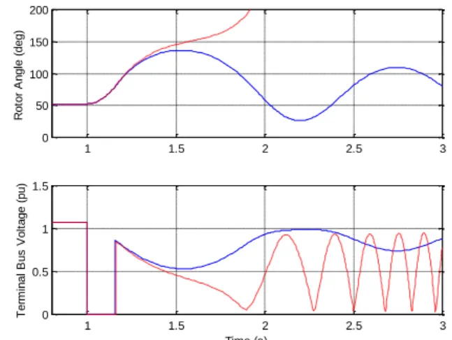
Coordinated Control of HVDC link, SVC (study case 2) In the second test, a simple test model with initial transfer level of 2GW and 500MW power on HVDC link (shown in

A trip of the central grid, trip of the PV system, and a three-phase short circuit isolating a generation and a load are simulated for stability studies of the hybrid power system

Ainsi, si l’exposé oral enregistré permet tout aussi bien aux étudiants d'apprendre ensemble, de diffuser le fruit de leur compréhension des contenus, soutenus par l'enseignant au

Plutôt que de voir des troubles et des symptômes à organiser en syndromes ou à additionner comme le fait pauvrement le DSM, A.Demaret repère des comportements et se pose la

les étudiants à l’AESS/Master à finalité didactique en biologie Marie-Noëlle HINDRYCKX Mélanie LASCHET Corentin POFFE Université de Liège.. A35 - DES IDÉES POUR LA

L’état de contrainte étant non uniforme, la résistance des assemblages a été exprimée par unité de longueur de soudure (N/mm). La rupture est observée dans la

They were compared to classic detectors such as matched pairs t-test, unpaired t-test, spectral method, generalized likelihood ratio test and estimated TWA amplitude within a

• Industrial Engineering students had extensive process knowledge and basic lean exposure. • Terminology sometimes a barrier (IE