Improved robust T-wave alternans detectors

HAL Id: hal-01101984

https://hal.archives-ouvertes.fr/hal-01101984

Submitted on 17 Apr 2016

HAL is a multi-disciplinary open access

archive for the deposit and dissemination of

sci-entific research documents, whether they are

pub-lished or not. The documents may come from

teaching and research institutions in France or

abroad, or from public or private research centers.

L’archive ouverte pluridisciplinaire HAL, est

destinée au dépôt et à la diffusion de documents

scientifiques de niveau recherche, publiés ou non,

émanant des établissements d’enseignement et de

recherche français ou étrangers, des laboratoires

publics ou privés.

Improved robust T-wave alternans detectors

Olivier Meste, Darius Janusek, S Karczmarewicz, A Przybylski, Michal Kania,

A Maciag, Roman Maniewski

To cite this version:

Olivier Meste, Darius Janusek, S Karczmarewicz, A Przybylski, Michal Kania, et al.. Improved robust

T-wave alternans detectors. Medical and Biological Engineering and Computing, Springer Verlag,

2015, 53 (4), pp.361-370. �10.1007/s11517-015-1243-5�. �hal-01101984�

(will be inserted by the editor)

The final publication is available at link

http://link.springer.com/article/10.1007%2Fs11517-015-1243-5

Improved robust T-wave alternans detectors

O. Meste · D. Janusek · S. Karczmarewicz · A. Przybylski · M. Kania · A. Maciag · R. Maniewski

Keywords: T-wave alternans; Detector; Electrocardiography; Ventricular Ar-rhythmia

O. Meste

Lab I3S, Universite de Nice-Sophia Antipolis, France D. Janusek

Nalecz Institute of Biocybernetics and Biomedical Engineering PAS, Warsaw, Poland S. Karczmarewicz

Warsaw Education Center CVG Medtronic Poland, Warsaw, Poland A. Przybylski

National Institute of Cardiology, Cardiac Arrhythmias Department, Warsaw, Poland M. Kania

Nalecz Institute of Biocybernetics and Biomedical Engineering PAS, Warsaw, Poland A. Maciag

National Institute of Cardiology, Cardiac Arrhythmias Department, Warsaw, Poland R. Maniewski

Abstract New statistical and spectral detectors, the modified matched pairs t-test, the extended spectral method and the modified spectral method, was pro-posed for T-wave alternans (TWA) detection gaining robustness according to trend and single frequency interferences. They were compared to classic detectors such as matched pairs t-test, unpaired t-test, spectral method, generalized likelihood ratio test and estimated TWA amplitude within a simulation framework and ap-plied to real data. The optimal detection threshold was selected by using a full Monte-Carlo simulation where signals, with and without alternans episodes, were corrupted by Gaussian noise with different power and single frequency interferences with different tones. All the combinations of noise and frequency were selected and

repeated 500 times in order to compute probability of detection (Pd) and the false

alarm probability (Pf a), providing ROC curves. The study group consisted of 50

patients with implantable cardioverter-defibrillator (age: 55.3±16.4; LVEF: 42.8

±15.5), who were paced (ventricular pacing) at 100 bpm. Two-minute recordings

were analyzed. The XYZ orthogonal lead system was used. The best performance was reached by using the modified matched pairs t-test (in comparison with the spectral method and other reference methods).

1 Introduction

The non-invasive risk stratification of life-threatening ventricular arrhythmias is nowadays of great clinical importance, especially for the prevention of sudden car-diac death (SCD) [1]. Currently, there is no generally accepted non-invasive SCD risk index [2]. The most important method employed to prevent SCD is the use of Implantable Cardioverter Defibrillator (ICD). The different parameters, such as: left ventricular ejection fraction (LVEF), ventricular late potentials, appearance of ventricular arrhythmic episodes in 24-hour Holter electrocardiograms, heart rate variability, T-wave abnormalities, QRS duration, repolarization duration interval, and QT variability, are used as the predictors of SCD, nonetheless their predic-tive value is still far from clinical needs [3]. Ventricular arrhythmia which can cause SCD is connected to the spatiotemporal heterogeneity of the repolarization process in the heart [4] which can be manifested as repolarization alternans. It arises from the beat to beat alternation of the action potential duration at the level of cardiac myocytes. This process can be spatially concordant if during one heart beat all ventricular cells have short action potential duration and during the next beat all ventricular cells have long action potential duration or discor-dant if at least one region is out of phase. Alternans can induce gradients of repolarization across the heart which are known substrates for cardiac arrhyth-mias [5], [6]. Repolarization alternans is seen on the surface electrocardiogram as T-wave alternans (TWA) which is a very promising electrocardiographic index of the increased risk of SCD [7], even though there is not yet definitive evidence that it can guide therapy [8]. The magnitude of TWA is assessed by the analysis of the beat-to-beat alternations in the shape, amplitude and timing of the ST segment,

T wave and U wave that repeats every other heart beat [9]. Clinical evidence link the appearance of TWA with inducible and spontaneous ventricular arrhythmias and mechanisms of arrhythmia generation [6]- [10]. The magnitude of TWA can be gained or attenuated by abrupt changes in heart rate or ectopic beats. The ischemia and extrasystoles may reverse the phase of alternans causing the devel-opment of discordant alternans and re-entrant arrhythmia. The microvolt T-wave alternans testing is considered as a tool which can help to identify candidates for ICD implantation [11]. The measurement of TWA is associated with the assess-ment of several parameters. The most common technique, which is connected to the basic TWA model, is the magnitude assessment [12]. A higher TWA ampli-tude reflects a greater SCD risk. Very important is the phase reversal when TWA changes its pattern from ABABAB to ABABBABA [13]. It could be a better pre-dictor of SCD than the elevated TWA magnitude, sustained arrhythmias induced in the electrophysiological test, or LVEF [14]. The shape of a TWA episode and its change to consecutive heart beats is another very important factor which should be considered during SCD risk assessment but its diagnostic value is still unclear. It was shown that a TWA episode following an abrupt heart rate change is not of diagnostic value and can be explained by the theory of restitution [15]. One other factor is the distribution of TWA within the T-wave, where the T-wave amplitude is of great importance [16]. The final one is the spatial distribution assessed by the number of ECG leads with the presence of TWA [17]. Usually, the standard 12-lead system is used for TWA assessment but also the XYZ orthogonal lead system as well as the optimal lead system selected from the body surface potential mapping (BSPM) are applied [18]. T-wave alternans is a heart rate dependent phenomenon. An increased heart rate leads to an amplified TWA amplitude, so

it can be induced even in normal subjects. To prevent false positive detections in medical diagnostics, a significant heart rate value was limited to 110 bpm. For a lower heart rate, the amplitude of TWA decreases and the detection becomes more complicated. For the TWA measurement at accelerated rates the stress test [19] or pacing is used [20]. TWA could also be measured without heart rate accelera-tion [21] in ambulatory electrocardiograms [22] and Holter recordings [23]. Many methods for TWA detection have been developed [9, 25]- [29]. The reliability of the detection process depends on the properties of the detectors and their suscep-tibility to noise interference and stationarity of the data [24]. Most of the TWA detectors consist of a filter, usually nonlinear, followed by a decision rule based on a threshold crossing. The determination of the optimal value of threshold level for decision making procedures is not trivial because its value is not adapted to any kind of interference types or levels. These interferences are typically the Gaussian or Laplacian noise, periodic components and slow trends [30]. Stress testing pro-duces a high level of single frequency interference as a product of pedaling when using ergometer. Respiration and body movements are also sources of periodic interferences that hinder the TWA detection.

Among the TWA detectors, in the Spectral Method (SM) [28] the T-wave

alternans signal is well separated from most of the interferences present in elec-trocardiographic signals. This method is a typical confidence interval computation

that uses normalized Fourier transform frequencies. In theSM method, all the

T-waves, typically 128 T-waves, are firstly aligned and processed, as depicted in fig. 1. Since the signals are sampled, this dataset corresponds to a matrix whose rows are the samples of the T-waves and the columns the different T-waves. Then, for each row the Fourier Transform is computed over 128 samples, providing an ensemble

of power spectrum which are finally averaged. In this averaged spectrum, the beat to beat fluctuation in the amplitude of the T-waves appears as the spectral peak at the frequency of 0.5 cycles ber beat and is positively detected according to the computation of a confidence interval for normally distributed random variable.

128 T-Waves

. .

.

. .

. .

. .

.

. .

. .

. .

.

. .

. .

Fig. 1 Schematic representation of the Spectral Method (SM) introduced in [28]

The magnitude of this peak is a direct marker of alternans. The suggested length of the data taken for the spectral analysis is 128 sample points corresponding to consecutive heart beats [28]. Shortening of the window is significant if TWA is changing its amplitude during the recording and it allows to track its dynamics. However, short windows increase the risk that random sequences will be falsely assigned as alternans. TWA is likely to be non-stationary under all measurement conditions. The disadvantage of this method is that it treats the T-wave alternans signal as a stationary sine wave with a constant amplitude and a phase, which is not true in general. This has significant implications for the selection and development of optimal measurement techniques. Among the well-known detectors such as

t-test [31], matched pairs t-t-test [31], generalized likelihood ratio t-test (glrt) [32],

or single frequency interference. For example, t-test based methods can reliably detect periodic changes in the T-wave amplitude but they are sensitive to trends in the data. In the same situation, matched pairs t-test is only slightly affected but without a TWA episode it will produce a false detection corresponding to low specificity.

In line of the aforementioned statistical and spectral approaches, we proposed new methods for T-wave alternans detection whose aim is to be robust according to pure tone interferences together with noise. In section 2, methods are introduced as extension of classic solutions. In section 2.1, the results of the sensitivity and specificity calculated in simulated and real data, obtained from 50 patients with ICD, were compared. Corresponding ROC curves and illustrative examples are displayed in section 3 where it was shown that the ventricular fibrillation risk stratification can be addressed by TWA detection. Discussion and conclusion close this paper.

2 Methods

In the following part of the paper, the new methods are described, and each of the T-wave alternans marker is defined. As it will be introduced in the following,

different sets of data will be processed. For the Spectral Method (SM), also called

alternans ratio in [28], a set of 128 consecutive T-waves are required and processed

globally. For the amplitudes comparison method (Amp), the original T-waves set

is split into consecutive subsets successively shifting, by one T-wave, a window of 16 T-waves. Thus, a set of 128 T-waves produced 128-16+1=113 consecutive subsets of 16 T-waves. For all the other methods the subsets of 16 T-waves are

also considered but they are subsequently processed in two different ways in order to supply single 16 values series to the detectors. In the first case, the average over time of every T-wave was calculated and the series was composed of the received results (processing labeled M). In the second case, the singular value decomposition (SVD) was computed and the series was built by using the first eigenvector instead of T- wave itself (processing labeled S). Finally, in the simulated data section the 16 values series are directly synthesized instead of T-waves and subsequent processings.

Unlike these processings, the sequence of values to be processed by SM is the

mean of the magnitude of all the Fourier transforms of the time correlated T- wave

samples, as depicted in fig. 1. ThenSM is defined by:

SM= F {¯ 0.5} − mean( ¯F {[0.35,0.45]})

std( ¯F {[0.35,0.45]}) (1)

According to the previous study [28], a patient is classified as alternans positive if the alternans ratio (AR) exceeds 3. It means that the power at alternans frequency (0.5 cycles per beat) is above noise level more than 3 times standard deviation of

noise estimated outside alternans frequency. In other words, SM defined by (1)

should be greater than a threshold equal to 3. Note that when using SM the

function ¯F {.} stands for the mean of the magnitude of all the Fourier transforms

as previously mentioned in Introduction section while for the following proposed

methods F {.} will be a single Fourier magnitude computed from processings M

or S. Because the range of frequencies suggested in [28] is not suitable for short length data analysis we propose a methodology of calculation which uses extended

frequency band for noise assessment (2) when 16 consecutive T-waves only are analyzed.

The Extended Spectral Method (ESM) proposed in [33] is also defined in the

spectral domain such as:

ESM= F {0.5} − mean(F {[0.25,0.5[})

std(F {[0.25,0.5[}) (2)

As for theSM, this definition corresponds to a confidence interval calculation

under the assumption of gaussianity. However, when data are contaminated by the single frequency interference, the spectrum exhibits spikes which makes the

gaussianity assumption invalid. Then, Modified Spectral Method (SM M) [33] was

proposed which is based on the averaging of data with the use of the median function (3).

SM M= F {0.5}

median(F {]0,0.5[}) (3)

The use of the median is meaningful when data are corrupted by spectral spikes due to periodic components. Then, without introducing a rigid model of the interferences, robustness is increased by using the median operator, known to be robust regards outliers in contrast to the mean. The preliminary study presented

in [33] shows the advantage of using SM M method. If we treat the problem of

TWA detection as a statistical issue, at least two tests appear to be suitable: t-test and matched pairs t-test. As it was shown in the introduction both of them fail in the presence of high elevated trends in signals with and without TWA. Matched pairs t-test is used to compare two population means (paired observations of the

same subject) and reduces inter-subject variability (since it makes comparisons between the same subject). Defined by:

pttest=ttest(seqodd− seqeven,0) (4)

, it is theoretically more powerful than unpaired t-test:

ttest=ttest(seqodd, seqeven) (5)

whereseqoddandseqevenstand respectively for the odd and even samples from

the data sequence . We proposed a novel statistical method which is Modified

Matched Pairs t-Test (M M P T) which is calculated according to the formula (4).

M M P T = 1

K K−1

X k=0

ttest(seqodd− circ(seqeven, k),0) (6)

where, K is the number of samples in the window of analysis. The function

circ(seqeven, k) shifts right values located in variable seqeven by k values in such

a way that the last value is moved to the first position. For instance, ifseqeven=

{a, b, c, d}then circ(seqeven,1) ={d, a, b, c}orcirc(seqeven,2) ={c, d, a, b}. In this method, Matched pairs t-test is calculated for the differences between odd sequence and every circular rotation of even sequence. The outcome of the method is the mean value calculated from the results of all the tests. Classical Matched pairs t-test performs badly when temporal trend is present in the data because of bad

specificity whereas the sensitivity is high. The aim of the circ() operator is to

the alternans feature. Here again without modeling the trend and its subsequent

substraction, robustness of the detection is improved compared topttest.

It is worth noticing that all these methods do not directly account for ampli-tudes of TWA for detection. In contrast, methods based on the TWA amplitude estimation provide a value where detection could be also applied. Along the same line of [12] we propose to use the following TWA energy estimation for comparison:

Ampi= 1 N N X n=1 ( ¯Todd,i(n)−T¯even,i(n))2 (7)

corresponding to the energy of the means (noted ¯T) difference of odd and even T

waves, wherenandistand for the T-wave sample number and T-waves block index,

respectively. Indeed, when the number of T-waves at disposal is large enough, the ensemble is splited in indexed blocks in order to track short duration alternans events. For instance, if the size of each T-wave block is 16 T-waves then the means are computed over 8 T-waves.

The last method tested in this work is theglrt[32]. This detector distinguishes

the two hypotheses (H0 andH1) applied to a model of observation where a

refer-ence T-wave is assumed identical along the observation and the interferrefer-ence is only

noise. The hypothesesH0 andH1 correspond to the lack or presence of alternans,

respectively. In [32] different types of noise are considered. This detector suffers from robustness in term of model departure.

Novel methods proposed in this paper defined in the time (M M P T) and

fre-quency (ESM,SM M) domains will be compared to the references ones (SM,ttest,

2.1 Application to simulated data

In order to gain in robustness, complete simulated data will be generated not only to compare methods but also to fix thresholds for subsequent processing. To this aim, synthetic observations are generated by adding gaussian noises and sinusoids, with different properties, to the alternans sequence. This processing is fully de-scribed and adapted to the analysis of real data. In order to stick to the properties of the observed interferences during experimental studies, the performance of all

the methods was assessed by 500 simulated positive sequencesseq1,idefined as:

seq1,i(n) = (−1)n+bi(n) +cisin(ωn); n= 1· · ·16 (8)

where it appears that the alternans sequence is corrupted by noise in addition to the single frequency interference. The window length was limited to 16 samples (or 16 beats according to T-wave analysis) in order to assess the performances with short duration alternans episodes. Note that for low frequencies, because the length of the window of analysis is 16 samples, the single frequency interference could be equivalent to a trend and it will be not seen as a periodic signal. The

Gaussian noise sequencesbi(n) were generated with 8 different standard deviations

σb = 0, 0.1, 0.3, 0.5, 0.7, 1, 1.5 , 2, the single frequency interference was chosen

from the set of 7 different frequencies ω (rad/s) = 0, 0.1, 0.3, 0.5, 0.7, 1, 1.7

andci is a Gaussian random variable with σc = 4. For all the possible values of

the pairs (σb, ω) a set of 500 TWA positive sequencesseq1,i (i = 1. . . 500) was

generated. Note that the simulations with only noise or only single frequency are

also provided by a proper selection ofσb andci . TWA negative sequencesseq0,i

Since the labels (alternans or no alternans) is known for each sequence from the up to 8x7x500 simulated sequences, the Receiver Operating Curves (ROC) can be computed by varying the threshold for detection. A detection threshold was selected which corresponds to the probability of false alarm equal to 5% (it is the risk of positive detection of 5 TWA sequences out of 100 when TWA is not present there).

2.2 Application to real data

Recordings of patients with ICD were analyzed with the use of all the methods. Electrocardiographic signals were recorded from the patients body surface. Six silver-silver chloride electrodes were positioned in the orthogonal XYZ lead config-uration. ECG signals were amplified (gain, 1000), filtered (bandwidth, 0.05 Hz to 500 Hz) and digitized (2 kHz sampling frequency, 22 bits resolution). Two minute recordings were made during the ventricular pacing at 100 bpm, during periodic control of the pacemaker, after implantation.

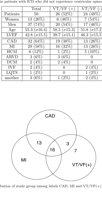
The study group consisted of 50 patients with ICD and with possible occur-rence of Ventricular Tachycardia/Ventricular Fibrillation (VT/VF) during the 10 years follow-up. Patients underwent the ICD implantation due to one of the fol-lowing conditions: Coronary Artery Disease (CAD), Myocardial Infarction (MI), Hypertrophic Cardiomyopathy (HCM), Dilated Cardiomyopathy (DCM), Long QT Syndron (LQTS), Arrhythmogenic Right Ventricular Dysplasia (ARVD), Id-iopathic Ventricular Fibrillation (IVF). The patients basic and detailed clinical data were shown in Table 1. For detailed analysis of clinical data, the repartition of the study group among CAD, MI and VT/VF(+) is given in fig. 2. CAD, MI

and VT/VF conditions play an important role for the risk stratification of life-threatening cardiac diseases and they are considered together with the presence of TWA [8], [35]. The study was conducted according to the Helsinki Declaration (1964). All participants provided informed consent prior to their participation.

Table 1 The study group clinical data (2). VT/VF (+): the patients with ICD who experi-enced ventricular tachycardia or ventricular fibrillation which occurred during their follow-up, VT/VF (-): the patients with ICD who did not experience ventricular episodes.

Total VT/VF (+) VT/VF (-) Patients 50 26 (52%) 24 (48%) Women 13 (26%) 6 (46%) 7 (54%) Men 37 (74%) 20 (54%) 17 (46%) Age 55.3 (σ16.4) 58.5 (σ15.3) 51.8 (σ17.2) LVEF 42.8 (σ15.5) 39.7 (σ15.1) 46.3 (σ15.5) CAD 32 (64%) 19 (38%) 13 (26%) MI 29 (58%) 16 (32%) 13 (26%) HCM 6 (12%) 1 (2%) 5 (10%) ARVD 3 (6%) 3 (6%) 0 DCM 2 (4%) 2 (4%) 0 IVF 2 (4%) 0 2 (4%) LQTS 1 (2%) 0 1 (2%) another 3 (6%) 1 (2%) 2 (4%) CAD MI VT/VF(+) 16 13 3 7

The ICD electrodes were used for pacing of the heart at the rate which was programmed in ICD device. The following procedures were applied, for X, Y, Z signal pre-processing :

– To localize T-waves in each heartbeat, the R peaks of the previously averaged

signal were detected by Pan-Tompkins algorithm [34]

– Baseline wander was eliminated by the use of cubic splines [36]

– T-wave locations were estimated using Bazett formula [37]. ECG signals

con-sisting of 128 T-waves with 310 ms time duration each were used.

– When it applies, in order to transform each segmented T-wave into a single

parameter for subsequent detection, they were averaged over time (labeled M) or projected onto their first singular vector (labeled S).

and for TWA detectorsM M P T,SM M,ESM,ttest,pttest,glrt:

– Parameters series were segmented by using a 16-values sliding window, for

instance consecutive M values.

– Filters (M M P T,SM M,ESM,ttest,pttest,glrt) were computed on each

seg-ment

– The filter outputs were compared to the detection threshold (individually

se-lected for each method based on the simulation study)

– Duration times of detection episodes were scored and the median value was

calculated. This value will be used for subsequent detection performance as-sessments that are ROC curves and ranksum tests.

In case ofSM method, the sequence of 128 values long does not allow a sliding

window processing. SM provides a single detection value for each lead. Finaly,

TWA is detected if the detection is positive in at least one lead.

For the TWA amplitude based detector the mean T wave operator is computed over 8 waves for both even and odd heart beat index, corresponding to the total of

16 waves forming thei’th T-waves block. Each processed T-wave block provides 3

Ampi values corresponding to expression (7) for the three leads. Since the initial

ensemble of T-waves is splited in several blocks (i= 1, . . . , I), the median function

is finally applied to all theAmpi(i= 1, . . . , I) to provide a single value for eachX,

Y,Zleads. To perform the comparison with other detectors not only the individual

lead values are computed but also the squared root, the minimum, the maximum,

the median and the mean of the three X, Y, Z values. These results are labeledAl,

with lcorresponding to how theX,Y, Z values are processed. These values will

be used for subsequent detection performance assessments that are ROC curves and ranksum tests.

3 Results

Sensitivity and specificity (alternatively Pd - probability of detection and Pf a

-probability of false alarm) were calculated with the simulated signals with and without TWA, providing Receiver Operating Curve (ROC) curves and subsequent Area Under the Curve (AUC). The three types of simulations were performed. At first, Gaussian noise was simulated and added to the signal. The obtained results for all the methods are shown in figure 3.

0 0.2 0.4 0.6 0.8 1 0.4 0.5 0.6 0.7 0.8 0.9 1 1−specificity sensitivity pttest ttest SMM ESM glrt MMPT

Fig. 3 Simulated ROC curves for all the analyzed methods. Only Gaussian noise is added in the model (8). The Gaussian noise sequences bi(n) were generated with different standard deviations σb= 0, 0.1, 0.3, 0.5, 0.7, 1, 1.5 , 2.

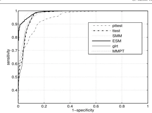
Next, single frequency interference were simulated and added to the signal. Obtained results are shown in figure 4.

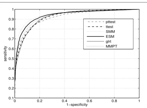
Finally, both Gaussian noise and single frequency interference were simulated and added to the signal. Obtained results for all methods are shown in figure 5.

Since the higher is the curve whatever the 1-specificity value, the higher is the performance of the corresponding detector, it is tedious to rank all the methods. However detection power of the methods can be compared by computing the Area Under the Curve (AUC) of each ROC curves. Comparing fig. 3 and 4, it is clear that the performances of the methods depend on the type of added interferences. For

instance, theESMperforms really better in the presence of sinusoidal interferences

compared to the noise case and the performance ofpttestdegrades strongly with

0 0.2 0.4 0.6 0.8 1 0.4 0.5 0.6 0.7 0.8 0.9 1 1−specificity sensitivity pttest ttest SMM ESM glrt MMPT

Fig. 4 Simulated ROC curves for analyzed methods. Only single frequency interference were added in the model (8). the single frequency interference was chosen from the set of frequencies ω (rad/s) = 0, 0.1, 0.3, 0.5, 0.7, 1, 1.7.

for each method which corresponded to the probability of false alarm equal to 5%. Respective values are shown in Table 2, in addition to the probability of detection

Pd and AUC.

Table 2 T-wave alternans detection AUC, thresholds and Pdfor Pf a=5%

Method AUC Threshold Pd

pttest 0.92 2.28 0.65 ttest 0.93 1.52 0.63 SM M 0.95 2.05 0.78 ESM 0.94 3.60 0.74 glrt 0.93 1.07 0.61 M M P T 0.94 1.63 0.67

Among the study group, 26 VT/VF positive patients exhibited ventricular tachycardia or fibrillation episodes. It is hypothesized that the presence of VF in the follow-up should correlate with the detection of TWA. The correlation of

0 0.2 0.4 0.6 0.8 1 0.1 0.2 0.3 0.4 0.5 0.6 0.7 0.8 0.9 1 1−specificity sensitivity pttest ttest SMM ESM glrt MMPT

Fig. 5 Simulated ROC curves for analyzed methods. Gaussian noise and single frequency interference were added in the model (8). Their statistical characteristics are identical to those used in figures 3 and 4.

TWA episodes with CAD and MI conditions is also analyzed separately but also

combining the three conditions, noted∩. These correlations are assessed by

com-puting first the AUC and secondly the ranksum test for comparison of mean. Note that this test has been selected because the normality test failed. The correspond-ing values are given in Table 3 where boldface means significant ranksum test for

means comparison (p <0.05).

In this table only AX andAmin, corresponding to lead X and the minimum

value (see section 2.1) , are given because otherAl failed to exhibit a significant

rank sum test, whatever the analyzed conditions. The presence of the VT/VF episodes in the follow-up was considered as a gold standard for decision making about increased risk to SCD. Additionally, the results of the analysis applied to

Table 3 AUC values for all the methods considering separately VT/VF, CAD, MI status and their intersection ∩. Left and right values correspond to M and S transformations, respectively. Bold face type is applied when ranksum test for means comparison is < 0.05

Method VT/VF CAD MI T M M P T 0.640.52 0.75 0.69 0.68 0.65 0.73 0.63 SM M 0.62 0.63 0.70 0.73 0.64 0.67 0.71 0.71 ESM 0.54 0.50 0.72 0.72 0.67 0.67 0.64 0.58 ttest 0.60 0.50 0.750.65 0.680.62 0.67 0.58 pttest 0.52 0.57 0.59 0.62 0.52 0.59 0.57 0.62 glrt 0.54 0.50 0.59 0.50 0.56 0.5 0.54 0.5 SM 0.45 0.58 0.60 0.6 AX 0.65 0.61 0.60 0.73 Amin 0.71 0.51 0.53 0.72

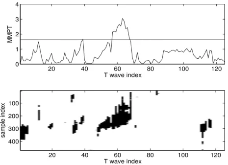
each time sample of the T-wave along the T-wave index axis are computed by the

M M P T methods and provided in figure 6 (lower part).

20 40 60 80 100 120 0 1 2 3 4 T wave index MMPT T wave index sample index 20 40 60 80 100 120 100 200 300 400

Fig. 6 Upper part: M M P T method output for a given patient (Y lead) where the sequence is the average in time of the T-wave (M pre-processing). Detection threshold is 1.63 (horizontal line). Lower part: M M P T method output for each time sample of the Twaves (in black -values > 1.63, in white - otherwise)

This example has been chosen because theSM failed, in contrast toM M P T,

the outcome of the method M M P T compared to the threshold of table 2. The corresponding segments where TWA was detected are plotted in black. In addition,

the upper part of this figure shows the result of the same analysis (M M P T),

applied to each T-wave but averaged in the time of the T-wave. It is clear that the localizations of the detected TWA are slightly different along the T-wave index axis and that detection appear mostly in the first half of the T- wave.

4 Discussion

The new methods (M M P T,SM M, ESM) as well as the well-known ones (ttest,

pttest,glrt,SM,Ampi) have been tested with the use of simulated data and real ECG recordings. All AUC differences in table 2 are significant after applying the test described in [38]. This test provides a p-value for the comparison of AUC cou-ples and a corresponding value below 0.05 is assumed significant in the following.

The results of the simulations showed that the best methods areSM M,ESMand

M M P T, confirmed by the corresponding AUC values equal to 0.95, 0.94 and 0.94.

In addition to thePd provided in table 2, the respective AUC equal to 0.92, 0.93

and 0.93 show that pttest,ttest andglrt failed to outperform other detectors. It

was not surprising because the requirements for the properties of the data that support these detectors were not fulfilled. The two first methods assume that the data are Gaussian and the last one relies on an inadequate model different from the simulated one. This is evidently reflected in figure 4 where only single frequency interference is considered as noise. This simulation stage provided thresholds for the application on real data. It is worth noticing that its aim was to reduce the overfitting of the presented methods with the real data for the detection

char-acterizations. Due to the fact that ESM, SM M and M M P T outperform other methods they were also compared with follow-up data connected with presence or absence of VT/VF episodes and CAD/MI conditions. Concerning VT/VF predic-tion, although their performance was not very high, the detection power assessed

by the AUC is the best forAmin (AUC=0.71), however not significantly, and the

worst is for SM method (AUC=0.45). The test for AUC comparison [38] shows

that significancy is only verified when comparingSMwithAX,Amin,M M P T and

SM M. In terms of AUC and ranksum test, the methods tend to be more accurate

when distinguishing CAD and MI groups. Meaning that TWA is more likely to be present in this category of subjects but not necessarily induces VT/VF episodes.

Notes that for both CAD and MI, the group (M M P T,SM M,ESM,ttest) exhibits

significant AUC differences compared to group (pttest, glrt,SM,AX,Amin) but

not inside the groups. Finally, combining all the conditions (∩) globally results

in good performance that concurs with other outcomes, confirming that in our dataset CAD/MI patients are prone to exhibit TWA.

It was foreseen better performances for SM M because of the simulation

out-comes, in contrast to the real data ones. This difference could be explained by the difficulty to model accurately real interferences in a simulation perspective. It is

worth noting that the performances ofSM M, the best detector from the

simula-tion scheme, are rather good with respect to AUC. In the case ofM M P T method,

the use of averaging of consecutive T-waves in the pre-processing stage (M) even increases the power of the detector. This is globally confirmed whatever the detec-tion method compared to the use of the SVD (S). According to the performance of

SMit could be hypothesized that TWA episodes were rarely long enough to make

is consider as a reference for TWA detection. The short duration of TWA is con-firmed by the threshold selection from fig. 6 equal to 4 a. u. in order to optimize the selectivity and specificity with respect to MMPT performances. Although this value is computed from our data set it could be suggested as a reference threshold for TWA detection. In summary, global results from table 3 seem to be in favor toM M P T method in term of AUC and ranksum test.

It is interesting to note that TWA amplitude based detectorAl(AXandAmin)

performed well for VT/VF and T, however not significantly better than others

exceptSM, but failed for CAD and MI because the ranksum tests are negative. It

probably means that the amplitude only is not enough to make the detector robust to interferences, impeding more complete detections. It is interesting to mention that unlike the other methods presented in this work, based on relative measures,

theAldetectors provide an rather good alternative as an absolute measure.

The overall low AUC for VT/VF prediction could be explained by the lack of real ground truth. In other words, it could be expected that patients suffering from VF should exhibit TWA but the presence of TWA does not necessarily mean that VF will occur, particularly when the transition from concordant to discor-dant TWA is not assessed [8]. This means that for a given level of sensitivity the specificity could be low.

5 Conclusions

It has been shown that alternatives exist while using the spectral domain as well as statistical tests. In contrast to this method, the proposed tools are applicable to short time windows which allow tracking of dynamic TWA episodes.

Robust-ness has been increased not only by using the median computed over the duration time of detections but also by fitting the detectors to the presence of spikes in the data spectrum or trends in the data sequences. Based on a fully simulated dataset, including different noise levels and single frequency interference, the pro-posed methods outperformed the classic ones. In addition, optimal thresholds were provided for a selected sensitivity. The methods were applied to real data where it appears that the detection of TWA episodes correlated with the existence of ven-tricular fibrillation and CAD/MI conditions. Although this detection is not related to a very high specificity, the proposed method is an adequate tool in comparison with the classic spectral method and amplitude based detector. The poor perfor-mance of the classical spectral method could be explained by a dynamic TWA pattern where short durations and changes of phase may hinder accurate detec-tions. The proposed methods proved that they are well designed for short time TWA episode detection and the use of averaging of T-waves in the pre-processing stage has the advantage of being less affected by misalignments of the T-waves. It was shown that this statistical test provides a complementary and computationally efficient solution to the alternans detection problem in surface ECG. Although the TWA amplitude estimation is addressed in this paper, it failed to outperform the proposed methods for extended detection.

Acknowledgements

This work was partially supported by the research project DEC-2011/01/B/ST7/06801 of the Polish National Science Centre.

Address for correspondence: O. MESTE Laboratoire I3S UNSA-CNRS 2000, route des lucioles Les Algorithmes - bt. Euclide B BP.121 06903 Sophia Antipolis - Cedex France meste@i3s.unice.fr

References

1. El-Sherif N, Khan A, Savarese J, Turitto G. Pathophysiology, risk stratification, and management of sudden cardiac death in coronary artery disease. Cardiology journal. 2010;17(1):4.

2. Christiaans I, Van Engelen K, Van Langen IM, Birnie E, Bonsel GJ, Elliott PM, et al. Risk stratification for sudden cardiac death in hypertrophic cardiomyopathy: systematic review of clinical risk markers. Europace. 2010;12(3):313-21.

3. Sastry AP, Narayan SM. Advanced Signal Processing Applications of the ECG: T-Wave Alternans, Heart Rate Variability, and the Signal Averaged ECG. Practical Signal and Image Processing in Clinical Cardiology. 2010:347-78.

4. Toure A, Cabo C. Effect of heterogeneities in the cellular microstructure on propaga-tion of the cardiac acpropaga-tion potential. Medical & Biological Engineering & Computing. 2012;50(8):813-25.

5. Selvaraj RJ, Picton P, Nanthakumar K, Mak S, Chauhan VS. Endocardial and epicardial repolarization alternans in human cardiomyopathy: evidence for spatiotemporal hetero-geneity and correlation with body surface T-wave alternans. Journal of the American College of Cardiology. 2007;49(3):338-46.

6. Pastore JM, Girouard SD, Laurita KR, Akar FG, Rosenbaum DS. Mechanism linking T-wave alternans to the genesis of cardiac fibrillation. Circulation. 1999;99(10):1385-94. 7. Qu Z, Xie Y, Garfinkel A, Weiss JN. T-wave alternans and arrhythmogenesis in cardiac

diseases. Frontiers in physiology. 2010;1.

8. Verrier RL, Klingenheben T, Malik M, El-Sherif N, Exner DV, Hohnloser SH, et al. Micro-volt T-wave alternans: Physiological basis, methods of measurement, and clinical utility-consensus guideline by international society for Holter and noninvasive electrocardiology. Journal of the American College of Cardiology. 2011;58(13):1309-24.

9. Naseri H, Pourkhajeh H, Homaeinezhad M. A unified procedure for detecting, quantifying, and validating electrocardiogram T-wave alternans. Medical & Biological Engineering & Computing. 2013;51(9):1031-42.

10. Arini PD, Baglivo FH, Martinez JP, Laguna P. Evaluation of ventricular repolarization dispersion during acute myocardial ischemia: spatial and temporal ECG indices. Medical & Biological Engineering & Computing. 2014:1-17.

11. Amit G, Rosenbaum DS, Super DM, Costantini O. Microvolt T-wave alternans and elec-trophysiologic testing predict distinct arrhythmia substrates: Implications for identifying patients at risk for sudden cardiac death. Heart Rhythm. 2010;7(6):763-8.

12. Nearing BD, Huang AH, Verrier RL. Modified moving average analysis of T-wave alternans to predict ventricular fibrillation with high accuracy. J Appl Physiol. 2002; 92:541-9. 13. Ghanem RN, Zhou X. Detection of T-Wave alternans phase reversal for arrhythmia

pre-diction and sudden cardiac death risk stratification. Google Patents; 2010.

14. Narayan SM, Smith JM, Schechtman KB, Lindsay BD, Cain ME. T-wave alternans phase following ventricular extrasystoles predicts arrhythmia-free survival. Heart Rhythm. 2005;2(3):234-41.

15. Janusek D, Kania M, Zaczek R, Zavala-Fernandez H, Maniewski R. A simulation of T-wave alternans vectocardiographic representation performed by changing the ventricular heart cells action potential duration. Computer Methods and Programs in Biomedicine, 2014. 114(1): p. 102-108.

16. Takasugi N, Kubota T, Nishigaki K, Verrier RL, Kawasaki M, Takasugi M, et al. Should T-wave alternans magnitude be corrected with T-wave amplitude in the ultra-short-term prediction of life-threatening cardiac arrhythmias? Europace. 2011;13(10):1512-3. 17. Janusek D, Fereniec M, Kania M, Kepski R, Maniewski R. Spatial distribution of T-wave

alternans. Computers in Cardiology, 2007; 2007: IEEE.

18. Nakai K, Takahashi S, Suzuki A, Hagiwara N, Futagawa K, Shoda M, et al. Novel algorithm for identifying T-wave current density alternans using synthesized 187-channel vector-projected body surface mapping. Heart and vessels. 2011;26(2):160-7.

19. Minkkinen M, Kahonen M, Viik J, Nikus K, Lehtimaki T, Lehtinen R, et al. Enhanced predictive power of quantitative TWA during routine exercise testing in the Finnish Car-diovascular Study. Journal of carCar-diovascular electrophysiology. 2009;20(4):408-15.

20. Dorenkamp M, Breitwieser C, Morguet AJ, Seegers J, Behrens S, Zabel M. T-Wave Al-ternans Testing in Pacemaker Patients: Comparison of Pacing Modes and Long-Term Prognostic Relevance. Pacing and Clinical Electrophysiology. 2011;34(9):1054-62. 21. Shusterman V, London B. Surge of T-wave alternans in the absence of heart-rate

accel-eration: A new predictor of sustained ventricular tachyarrhythmias in patients with low ejection fraction? Heart Rhythm. 2012;9(11):1920.

22. Li-na R, Xin-hui F, Li-dong R, Jian G, Yong-quan W, Guo-xian Q. Ambulatory ECG-based T-wave alternans and heart rate turbulence can predict cardiac mortality in patients with myocardial infarction with or without diabetes mellitus. Cardiovascular Diabetology. 2012;11:104.

23. Sakaki K, Ikeda T, Miwa Y, Miyakoshi M, Abe A, Tsukada T, et al. Time-domain T-wave alternans measured from Holter electrocardiograms predicts cardiac mortality in patients with left ventricular dysfunction: a prospective study. Heart Rhythm. 2009;6(3):332-7. 24. Janusek D, Kania M, Zaczek R, Zavala-Fernandez H, Zbiec A, Opolski G, et al. Application

of wavelet based denoising for T-wave alternans analysis in high resolution ECG maps. Meas Sci Rev. 2011;11(6):181-4.

25. Martinez JP, Olmos S. A robust T wave alternans detector based on the GLRT for Lapla-cian noise distribution. Computers in Cardiology, 2002.

26. Meste O, Janusek D, Maniewski R. Analysis of the T wave alternans phenomenon with ECG amplitude modulation and baseline wander. Computers in Cardiology, 2007. 27. Nearing BD, Huang AH, Verrier RL. Dynamic tracking of cardiac vulnerability by complex

demodulation of the T wave. Science (New York, NY). 1991;252(5004):437.

28. Rosenbaum DS, Jackson LE, Smith JM, Garan H, Ruskin JN, Cohen RJ. Electrical al-ternans and vulnerability to ventricular arrhythmias. New England Journal of Medicine. 1994;330(4):235-41.

29. Zareba W, Badilini F, Moss AJ. Automatic detection of non-visible T-wave alternans from three-channel Holter recordings. Journal of the American College of Cardiology. 1995;25(2):409A.

30. Janusek D, Pawlowski Z, Maniewski R. Evaluation of the T-wave alternans detection methods: a simulation study. Anatol J Cardiol 2007;7 Suppl 1:116-9.

31. Srikanth T, Lin D, Kanaan N, Gu H. Presence of T-wave alternans in the statistical con-text. A new approach to low amplitude alternans measurement. Computers in Cardiology, 2002; 2002: IEEE.

32. Martinez JP, Olmos S. Methodological principles of T wave alternans analysis: a unified framework. IEEE Transactions on Biomedical Engineering, 2005;52(4):599-613.

33. Meste O, Janusek D, Kania M. A New Robust T Wave Alternans Detector and its Thresh-old Optimization. A New Robust T Wave Alternans Detector and its ThreshThresh-old Optimiza-tion. Computers In Cardiology, 2012.

34. Pan J, Tompkins WJ. A real-time QRS detection algorithm. IEEE Transactions on Biomedical Engineering, 1985(3):230-6.

35. Burattini L, Zareba W, Rashba EJ, Couderc JP, Konecki J, Moss AJ. ECG features of microvolt T-wave alternans in coronary artery disease and long QT syndrome patients. Journal of Electrocardiology. 1998;31 Suppl:114-20.

36. Meyer C, Keiser H. Electrocardiogram baseline noise estimation and removal using cubic splines and state-space computation techniques. Computers and Biomedical Research. 1977;10(5):459-70.

37. Bazett H. An analysis of the time-relations of electrocradiograms. Annals of Noninvasive Electrocardiology. 2006;2(2):177-94.

38. DeLong E, DeLong D, Clarke-Pearson D. Comparing the areas under 2 or more cor-related receiver operating characteristic curves - a nonparametric approach. Biometrics 1988;44(3):837-45.