POLYTECHNIQUE MONTRÉAL
affiliée à l’Université de MontréalControl Strategies for Standing Column Wells in a Cold Climate
CAMILLE BEURCQ
Département de génie mécanique
Mémoire présenté en vue de l’obtention du diplôme de Maîtrise ès sciences appliquées Génie mécanique
Mai 2019
POLYTECHNIQUE MONTRÉAL
affiliée à l’Université de MontréalCe mémoire intitulé :
Control Strategies for Standing Column Wells in a Cold Climate
présenté par Camille BEURCQ
en vue de l’obtention du diplôme de Maîtrise ès sciences appliquées a été dûment accepté par le jury d’examen constitué de :
Michel BERNIER, président
Michaël KUMMERT, membre et directeur de recherche Philippe PASQUIER, membre et codirecteur de recherche Massimo CIMMINO, membre
DEDICATION
‘Almost every way we make electricity today, except for the emerging renewables and nuclear, puts out CO2. And so, what we’re going to have to do at a global scale, is create a new system. And so, we need energy miracles.’
TED conference, 2010, Bill Gates
‘Chaque génération, sans doute, se croit vouée à refaire le monde. La mienne sait pourtant qu’elle ne le refera pas. Mais sa tâche est peut-être plus grande. Elle consiste à empêcher que le monde se défasse’
ACKNOWLEDGEMENTS
Pour commencer, je voudrais remercier mon directeur de recherche, le professeur Michaël Kummert pour son soutien constant et son regard vif et précis sur mon travail. Il a su m’accompagner et faire évoluer ma réflexion grâce à ses précieux conseils toujours très pertinents en partageant ses connaissances malgré une charge de travail conséquente. Je suis très reconnaissante d’avoir pu bénéficier de son encadrement de qualité, de son expertise, et de ses nombreux encouragements pendant ces deux ans de collaboration.
Mes remerciements s’adressent aussi particulièrement à mon codirecteur, le professeur Philippe Pasquier, dont les conseils, le temps accordé et l’expertise technique ont permis à ce projet de voir le jour. Je le remercie pour son soutien, sa bonne humeur, mais aussi sa patience lors de nos rencontres qui m’ont toujours (re)motivée.
Je remercie aussi Alain Nguyen qui a mis à ma disposition le modèle du puits à colonne permanente élaboré pendant son doctorat et qui est à la base de la recherche présentée dans ce mémoire. Un grand merci à tous mes collègues du bee-lab pour nos diverses discussions, scientifiques ou non, particulièrement le bureau 317 : Sam, Alex, Louis, Gregor, Walid, Kun et Florent.
Enfin j’aimerais remercier mille fois mon équipe de rugby qui m’a permis de retrouver et de garder un bel équilibre, au prix de quelques bleus, et qui m’a ouvert les portes d’une nouvelle passion et d’un bonheur intense et partagé, comme une nouvelle famille.
Merci à mes autres amis de poly, et aux Canadians colors, ceux qui sont encore là et ceux qui sont rentrés, chacun m’a apporté quelque chose d’essentiel : des rires, de belles discussions ou de merveilleux souvenirs.
Enfin, même s’ils sont loin, un grand merci à ma famille, particulièrement mes parents et ma sœur pour leur soutien indéfectible et l’amour qu’ils me portent au quotidien.
Enfin, j’aimerais adresser ma plus sincère gratitude à l’Institut de l’Énergie Trottier (IET) pour le soutien financier octroyé à ce projet. Ce travail de recherche n’aurait pas été possible sans la participation financière de l’IET.
RÉSUMÉ
Les puits à colonne permanente sont des échangeurs géothermiques relativement profonds qui ont pour particularité d’utiliser directement l’eau souterraine comme fluide caloporteur. L’eau est généralement pompée à la base du puits grâce à une pompe submersible jusqu’à un échangeur à plaques. Ce dernier fait le lien entre la boucle d’eau souterraine et la boucle d’eau du bâtiment sur laquelle sont connectées des pompes à chaleurs décentralisées qui assurent le chauffage et la climatisation du bâtiment. L’eau est ensuite réinjectée en haut du puits sous le niveau dynamique à l’aide d’un tuyau de réinjection. Avant d’être réinjectée dans le puits, jusqu’à 30% de l’eau souterraine peut être déviée vers un puits d’injection (ou une autre destination) ce qui a pour effet d’attirer de l’eau, à une température proche de celle du sol non perturbé, à travers les fractures du sol dans le puits à colonne permanente et ainsi d’augmenter sa performance thermique. Ce processus est aussi appelé ‘saignée’. Ce type d’échangeur implique des forages relativement longs, mais leur efficacité thermique permet de réaliser des économies par rapport à des puits en boucles fermée. La boucle d’eau du bâtiment comporte aussi des auxiliaires de chauffage et de refroidissement qui prennent le relai quand l’échangeur souterrain ne peut répondre à la demande du bâtiment, particulièrement lors des pointes de demande.
La consommation énergétique de ces systèmes provient des pompes à chaleur, de l’énergie de pompage, et de l’énergie consommée par les systèmes auxiliaires. Les coûts d’opération peuvent aussi être influencés par la pointe de puissance appelée par le système. D’un autre côté, la saignée implique des impacts environnementaux et peut être reliée à des contraintes d’opération techniques et légales, et il est donc intéressant de limiter le volume d’eau saignée du puits.
Le but de cette recherche est d’explorer et de recommander des stratégies de contrôle des bâtiments équipés de puits à colonne permanente pour le pompage, la saignée, les consignes de température du bâtiment et des systèmes auxiliaires, dans le but d’améliorer l’efficacité énergétique du système et les coûts d’opération, tout en limitant le volume d’eau souterraine saignée.
Ce travail de recherche comporte le développement d’un modèle de bâtiment de bureau détaillé en plusieurs zones chauffées et climatisées par des pompes à chaleur décentralisées. Le modèle a été réalisé avec le logiciel TRNSYS pour la partie bâtiment tandis que l’échangeur géothermique est modélisé dans Matlab. Une étude des pertes de charge dans la boucle d’eau souterraine a été
réalisée pour une meilleure précision de l’évaluation des stratégies de pompage de façon à prendre en compte l’impact de la saignée sur l’énergie de pompage.
La revue de littérature a permis d’identifier un scénario de référence qui regroupe les pratiques et recommandations pour le contrôle de système qui servira pour comparer l’impact des stratégies testées. Les simulations réalisées se séparent en trois grandes catégories : les stratégies de pompage, de saignée et de contrôle du bâtiment.
Les stratégies de pompages implémentées ont montré l’intérêt de l’utilisation des pompes submersibles à vitesse variable afin de contrôler le débit de pompage en fonction de la charge sur la boucle d’eau du bâtiment. La meilleure stratégie identifiée permet des économies de 8 % du coût d’opération par rapport au scénario de référence avec un volume d’eau saignée réduit ou identique. Les stratégies de saignée ont montré qu’à débit de saignée constant, il n’était pas nécessaire d’aller au-dessus de 15% de débit saigné. La combinaison de stratégies simples de saignée avec la meilleure stratégie de pompage permet d’obtenir différents points d’opération selon les contraintes retenues pour le volume d’eau saignée : dans une large plage d’opération, les résultats montrent une diminution quasi linéaire des coûts d’opération en fonction du volume saigné, mais la combinaison des stratégies proposées permet ici encore une amélioration significative du coût d’opération par rapport au scénario de référence, à volume d’eau de saignée égal. Des stratégies de contrôle du débit de saignée évoluant par rapport à la charge ont montré un intérêt lorsqu’elles sont basées sur l’évolution de la charge future afin de préparer les puits à répondre à une demande importante comme lors de la reprise le matin. Cependant, les économies engendrées par ces stratégies ‘prédictives’ sont faibles et semblent difficilement justifier le niveau de complexité introduit. Enfin, on a aussi voulu étudier le bâtiment dans son ensemble au travers des stratégies de contrôle du bâtiment en lui-même. Les simulations ont démontré que les coûts et l’énergie consommée sont très sensibles au choix de la consigne de l’auxiliaire et peuvent être facilement améliorés grâce à l’utilisation d’un profil de consigne évitant les reprises matinales rapides pour les températures du bâtiment. Ces deux paramètres ont un impact significatif sur la performance globale, et doivent donc être optimisés en même temps que les paramètres de pompage et de saignée.
ABSTRACT
Standing column wells (SCWs) are a type of ground heat exchanger which relies on relatively deep wells and uses groundwater directly as the heat transfer fluid. The groundwater is generally pumped at the bottom of the well with a submersible pump to a plate heat exchanger. This heat exchanger is the connection between the ground loop and the building loop which supplies the source side of distributed heat pumps providing heating and cooling to the building. The groundwater is then reinjected at the top of the well below the dynamic level of the aquifer with a rejection pipe. Before being reinjected, up to 30% of the groundwater may be diverted into an injection well (or another destination). This has the effect to attract groundwater at a temperature close to the undisturbed ground temperature from the ground fractures in the aquifer into the standing column well, which will increase its thermal performance. This process is also called ‘bleed’. Although this type of ground heat exchanger relies on relatively deep wells, their high heat exchange capacity can lead to cost savings compared to closed-loop systems. SCW systems also include auxiliary devices for heating and cooling, which are used when ground heat exchanger is not sufficient to meet the building load, especially during peak periods.
The energy use of SCW systems comes from the heat pumps, the submersible pump, and auxiliary heating and cooling devices. Operative costs are also influenced by the peak power demand of the system. On the other hand, bleed can be associated to environmental impacts and subject to technical and legal constraints, so there is an interest to limit the volume of groundwater bled. The goal of this research is to design and assess control strategies of the building for : pumping, bleed, and building and auxiliary setpoint temperatures with the aim of improving the overall energy efficiency and operative costs while minimizing the volume of groundwater bled.
The work performed includes the development of a detailed model of an office building that includes fifteen thermal zone heated and cooled by decentralized heat pumps. The building and HVAC system are modelled in TRNSYS while the ground heat exchanger is modelled in Matlab. A detailed assessment of the head losses in the ground loop with and without bleed was performed in order to accurately represent the impact of bleed on the pumping energy needs, as this is a key aspect of the overall control optimization.
Through the literature review, a ‘good practice’ scenario was identified. This scenario combines typical practice and recommendations regarding SCW systems operation. Simulations are then performed to assess the impact of different control assumptions on the system performance, compared to this reference scenario. The simulations are separated in three main categories : pumping, bleed and building (including auxiliary) control strategies.
The pumping control strategies implemented showed the interest of variable speed submersible pump so that the pumping flow rate evolves as a function of the load on the building loop. The best strategy delivers up to 8 % savings in operating costs compared to the good practice scenario, with an equivalent or reduced volume of groundwater bled. The bleed control strategies showed that when implementing a constant bleed flow rate, going over a 15% bleed ratio is not beneficial. The combination of simple bleed ratio control strategies with the best pumping strategy allows to obtain different operating points depending on the selected constraints regarding the volume of groundwater bled: over a large operating range, operating costs decrease quasi-linearly with an increase of the volume bled. Here again, the combination of proposed strategies delivers significant operating cost savings with an equivalent volume of groundwater bled. The implementation of linear control for bleed flow rate shows an interest when it is based on the future load predicted on the building loop. These control strategies help the well prepare for large load demand especially before the morning start. However, the cost savings with those ‘predictive’ strategies are modest, especially when compared to the added complexity of implementation, and they may not be justified in the studied case. Finally, this work aimed at studying the building as a global system specifically regarding the zone setpoint temperatures and the auxiliary heating setpoint. The simulations showed that the costs savings and energy consumption are very sensitive to the choice of the auxiliary temperature setpoint. The performance is also significantly better if a “smoother” setpoint profile is used for the building zones, with long ramps to recover from the night setback/startup. These two parameters have a large impact on the overall system performance and must be optimized together with the control parameters for pumping and bleed ratio.
TABLE OF CONTENTS
DEDICATION ... III ACKNOWLEDGEMENTS ... IV RÉSUMÉ ... V ABSTRACT ...VII TABLE OF CONTENTS ... IX LIST OF TABLES ... XIV LIST OF FIGURES ... XVI LIST OF SYMBOLS AND ABBREVIATIONS... XX LIST OF APPENDICES ... XXVINTRODUCTION ... 1
1.1 Objectives ... 4
1.2 Master Thesis Outline ... 4
LITERATURE REVIEW ... 6
2.1 Standing Column Wells ... 6
2.2 Simulation Models of Standing Column Wells... 8
2.2.1 Analytical Models ... 8
2.2.2 Numerical Models ... 9
2.2.3 Thermal Resistance and Capacity Models ... 10
2.3 Installations and Operational Data ... 10
2.3.1 Capacity and Sizing ... 11
2.3.2 Pumping flow rate ... 11
2.3.3 Case Studies Presenting Operating Data ... 12
2.4.1 Bleed Impacts and Issues ... 15
2.4.2 Control Strategies for Bleed ... 15
2.5 Summary ... 18
SYSTEM MODELLING: BUILDING, HVAC AND GROUND LOOP ... 20
3.1 The Building ... 21 3.1.1 Geometry ... 21 3.1.2 Building Envelope ... 22 3.1.3 Internal Gains ... 23 3.1.4 Infiltration ... 25 3.1.5 Ventilation ... 26
3.1.6 Heating and Cooling Setpoint Temperature ... 27
3.1.7 Internal Mass ... 28
3.1.8 Other Energy Uses ... 29
3.1.9 Ground Coupling ... 30
3.1.10 Annual Building Energy Loads ... 31
3.2 Building Loop ... 32
3.2.1 Heat Pumps ... 33
3.2.2 Outdoor Air ... 35
3.2.3 Building Loop Variable-Speed Pump ... 36
3.2.4 Auxiliary Heating and Cooling Devices ... 37
3.2.5 Pipes ... 37
3.3 Ground Loop ... 37
3.3.1 SCW Model ... 37
3.3.3 Drawdown in SCW and Impression in Injection well... 41
3.3.4 Pumping ... 42
3.3.5 Heat Exchanger ... 42
3.4 Operating Cost Assessment ... 42
3.4.1 Hydro-Québec – Rate M ... 42
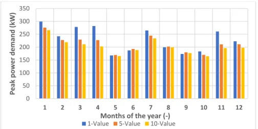
3.4.2 Peak Power Demand Calculation ... 43
3.4.3 Peak Power Demand and On/Off Control Effect ... 43
3.5 Reference Scenarios ... 44
HEAD LOSS AND IMPAC ON PUMPING POWER ... 47
4.1 System Configuration ... 47
4.2 Head loss Calculation and Assumptions ... 50
4.2.1 Fluid properties ... 51
4.2.2 Pipe head loss ... 51
4.2.3 Singular Head Loss in Elbows and Valves ... 53
4.2.4 Heat Exchanger Head Loss ... 53
4.2.5 Drawdown and Impression ... 55
4.3 Pump Hypothesis ... 55
4.4 Pumping Power Assessment ... 56
PUMPING FLOW RATE CONTROL STRATEGY ... 59
5.1 Constant Pumping Strategies ... 59
5.1.1 Simulations and Scenarios ... 59
5.1.2 Behavior During Peak Heating Day ... 59
5.1.3 Annual Simulation Results ... 62
5.2.1 Simulation and Scenarios ... 65
5.2.2 Constant versus Linear Pumping Strategy during Peak Heating Day ... 66
5.2.3 Annual Simulation Results ... 69
5.3 Linear Control Thresholds Sensitivities ... 71
5.3.1 Simulations and Scenarios ... 71
5.3.2 Annual Simulation Results ... 72
5.4 Conclusion ... 73
BLEED FLOW RATE CONTROL STRATEGY ... 75
6.1 Control Strategies ... 75
6.1.1 Building Load for Predictive Strategies ... 77
6.2 System Behavior on the Peak Heating Day ... 78
6.2.1 Control Strategies with Constant Bleed Ratios (1.a to 1.e) ... 78
6.2.2 Linear Control for Bleed Flow Rate ... 81
6.2.3 Predictive Control ... 84
6.3 Annual Results ... 87
6.4 Conclusion ... 89
BUILDING CONTROL STRATEGIES AND OVERALL RESULTS DISCUSSION………… ... 91
7.1 Building Heating and Cooling Setpoints ... 91
7.2 Auxiliary Setpoint Temperature ... 93
7.3 Overall Discussion of Control Strategies ... 96
CONCLUSION ... 98
8.1 Recommendations ... 100
LIST OF TABLES
Table 2.1: Summary of the data collected on SCWs systems. (The parentheses contain the range
reported in the questionnaire.) ... 11
Table 3.1: Summary of the different walls, their layers and overall resistance ... 22
Table 3.2: Characteristics of massive layers ... 23
Table 3.3: Characteristics of massless layers ... 23
Table 3.4: Internal gains ... 24
Table 3.5: Values for factor C in infiltration regime types ... 25
Table 3.6: Coefficient for wind approximation at building height ... 26
Table 3.7: Yearly energy load for the building ... 32
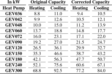
Table 3.8: Table of heat pumps capacities in cooling and heating before and after fan correction ... 33
Table 3.9: Overview of the heat pump sizing ... 34
Table 3.10 :Operative Flow rate of the Heat Pumps ... 36
Table 3.11: Parameters of the SCW. ... 39
Table 3.12: Inputs and outputs of type 155. ... 40
Table 3.13: Characteristics included in drawdown and impression modelization ... 42
Table 4.1 : Summary of the parts considered in head loss calculation ... 50
Table 4.2: Coefficient K for head loss calculation ... 53
Table 4.3: Size of the plate heat exchanger used ... 54
Table 4.4: Operation data of the heat exchanger ... 55
Table 4.5: Values for s, I and D considered for head loss observation when operating at 214 L/min ... 55
Table 5.1 : Summary of energy, power and total costs for constant control ... 65
Table 5.2: Energy, power and total costs for linear control ... 71
Table 5.3 : Tested thresholds ... 72
Table 5.4: Energy, power and total costs for different thresholds ... 72
Table 6.1: Summary of the control strategies implemented for bleed ratio ... 76
Table 6.2: Summary of pumping energy and groundwater bled for no bleed, 10% and 25% bleed ratio during the heating peak day ... 81
Table 6.3 : Summary of the cases tested in this sensitivity study ... 83
Table 6.4: Summary of HVAC costs, energy and peak power demand of the building and groundwater volume for a yearly simulation ... 84
Table 7.1: Peak power demand, annual energy use and costs for different setpoint profiles ... 92
LIST OF FIGURES
Figure 1.1: Layout of a closed-loop (a) and open-loop (b) ground heat exchanger ... 2
Figure 2.1: Illustration of a standing column well installation ... 7
Figure 2.2: Three level bleed control and ON-OFF sequence ... 18
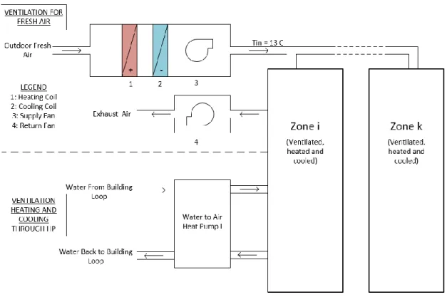
Figure 3.1: System simulated ... 20
Figure 3.2: Building dimensions ... 21
Figure 3.3 : 3D view of the building ... 21
Figure 3.4: Schedule for light gains ... 24
Figure 3.5: Schedule for equipment gains ... 24
Figure 3.6: Schedule for occupancy from NECB 2011 ... 24
Figure 3.7: Schedule for fan operation ... 26
Figure 3.8: Ventilation for a zone i in the detailed simulation ... 27
Figure 3.9: Constant setpoint profile for cooling and heating ... 28
Figure 3.10: NECB setpoint profile for cooling and heating ... 28
Figure 3.11: Ramping setpoint profile for cooling and heating ... 28
Figure 3.12: Schedule for Service Water Heating ... 29
Figure 3.13: Schedule for Elevators Use ... 30
Figure 3.14: Floor slab boundary temperatures for setpoint in configuration 4 ... 31
Figure 3.15: Daily mean and maximum power for heating and cooling ... 31
Figure 3.16: Heat pump in heating mode (left) and cooling mode (right) ... 35
Figure 3.17: Illustration of the resistance and capacity distribution for one node from Nguyen et al. (2015a) ... 38
Figure 3.18: SCW coaxial geometry and the radial thermal resistances associated from Nguyen et al. (2015a) ... 39
Figure 3.19: Graph of the monthly peak power demand calculated for 15-min, and by averaging 5
and 10 timestep values. ... 44
Figure 3.20: Annual operating cost vs. annual volume of groundwater bled ... 45
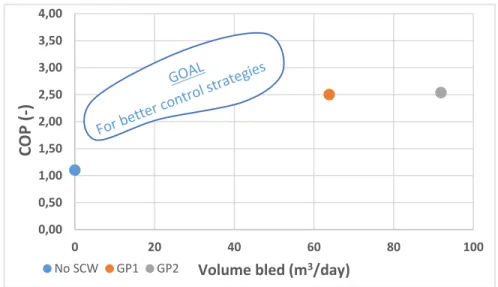
Figure 3.21: Annual COP vs. annual volume of groundwater bled ... 46
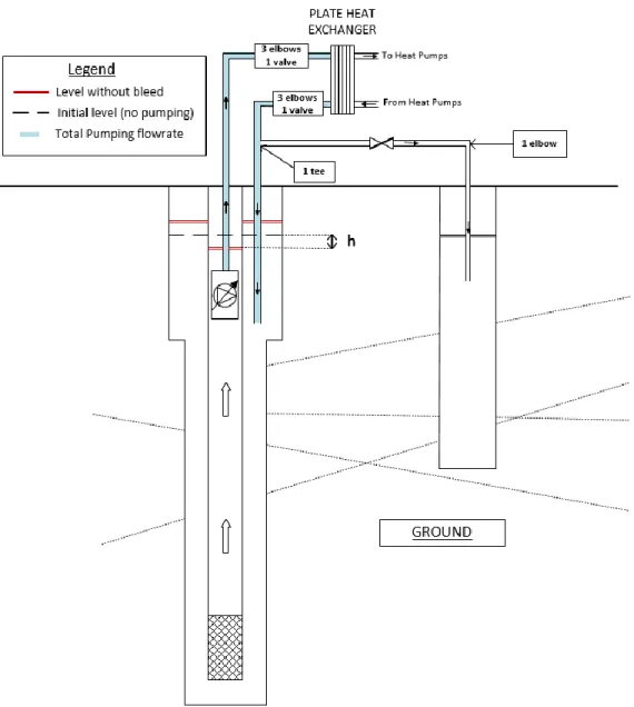
Figure 4.1: Installation configuration working without bleed for a groundwater withdrawal at the bottom of the SCW ... 48
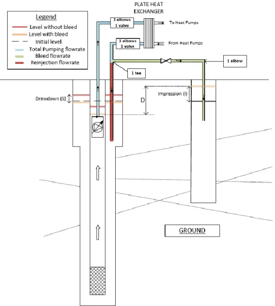
Figure 4.2 :Installation configuration working with bleed for a ground water withdrawal at the bottom of the SCW ... 49
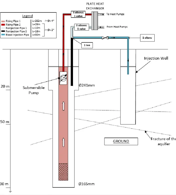
Figure 4.3: Pattern of each pipes and their dimension considered in head loss calculation ... 52
Figure 4.4: Head loss as a function of the flow rate with a 10% bleed rate and a ... 57
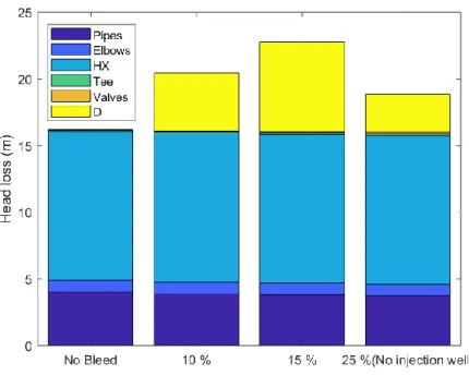
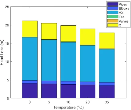
Figure 4.5: Head loss for various bleed scenarios for a total flow rate of 214 L/s and 5 °C ... 57
Figure 4.6: Head loss as a function of temperature for 214 L/s and a bleed rate 10 % ... 58
Figure 5.1: Inlet and outlet temperature of a SCW for 1.5 and 3.5 GPM/ton ... 60
Figure 5.2: Energy exchanged on the source side of the heat exchanger for 1.5 and 3.5 GPM/ton ... 61
Figure 5.3: Heating energy of the auxiliary system for 1.5 and 3.5 GPM/ton ... 61
Figure 5.4: COP of the heat pumps for the four models implemented at two flow rates ... 62
Figure 5.5: Annual energy used for heating and cooling ... 64
Figure 5.6: Annual maximum peak power ... 64
Figure 5.7: Annual operation costs for the medium office building ... 64
Figure 5.8: Groundwater volume bled ... 64
Figure 5.9: Linear flow rate control strategy ... 66
Figure 5.10: Pumping flow rate on the source side of the heat exchanger for constant and linear controls ... 67
Figure 5.12: Heating energy transferred for constant and linear control ... 68
Figure 5.13: Heating auxiliary energy for constant and linear controls ... 68
Figure 5.14: Annual energy consumed ... 70
Figure 5.15: Annual peak power demand ... 70
Figure 5.16: Annual costs for the medium office building ... 70
Figure 5.17: Groundwater volume bled ... 70
Figure 5.18 : Compared linear control variables ... 72
Figure 5.19: Annual operating cost vs. annual volume of groundwater bled ... 73
Figure 5.20: Annual COP vs. annual volume of groundwater bled ... 74
Figure 6.1: Bleed ratio linear control with minimum (orange) without minimum (blue) ... 77
Figure 6.2: Inlet and outlet temperature of SCW for No bleed (1.a), 10% (1.c) and 25% (1.e) bleed ratio ... 79
Figure 6.3: Heating auxiliary power for No bleed (1.a), 10% (1c) and 25% (1.e) bleed ratio ... 79
Figure 6.4: Heat transferred on source side of HX for No bleed (1.a), 10% (1.c) and 25% (1.e) bleed ratio ... 79
Figure 6.5: COP of heat pumps for the four models implemented in a no bleed and 25% bleed ratio scenario ... 80
Figure 6.6 : Illustration of the bleed flow rate implemented in configurations 1.c, 2.a and 2.b during peak heating day. ... 82
Figure 6.7: Inlet and outlet temperature of SCW for 1.c, 2.a and 2.b configuration ... 82
Figure 6.8 : Heating auxiliary power for configurations 1.c, 2.a and 2.b ... 83
Figure 6.9 : Heat transferred on source side of HX energy for configurations 1.c, 2.a and 2.b .... 83
Figure 6.10: Illustration of the parameters tested in the sensitivity study for linear control of bleed flow rate ... 83
Figure 6.12 : Inlet and outlet temperature of the SCW for 2.b, 3.a and 4.a configuration ... 86
Figure 6.13 : Heating auxiliary energy for 2.b, 3.a and 4.a configurations ... 87
Figure 6.14 : Annual results for HVAC costs (a) and groundwater bled (b) for all configurations ... 88
Figure 6.15 : Annual operating cost vs. annual volume of groundwater bled ... 90
Figure 6.16 : Annual COP vs. annual volume of groundwater bled ... 90
Figure 7.1: NECB setpoint profile ... 92
Figure 7.2: Constant setpoint profile ... 92
Figure 7.3: Ramping setpoint profile ... 92
Figure 7.4: Impact of auxiliary heating setpoint temperature on peak power demand and SCW temperatures ... 94
Figure 7.5: Annual operating cost vs. annual volume of groundwater bled ... 97
LIST OF SYMBOLS AND ABBREVIATIONS
List of Abreviations ASHRAE COP EWT GHE GPM GSHP HDPE HP HVAC HX LWT NCBE PVC SCW SHGC SWH TESS TRCM TRNSYS USA USDOEAmerican Society of Heating, Refrigerating and Air-Conditioning Engineers Coefficient of performance
Entering water temperature (to the heat pumps) Ground Heat Exchanger
Gallons per minutes Ground Source Heat Pump High Density Polyethylene Heat Pump
Heating, Ventilation and Air Conditionning Heat Exchanger
Leaving water temperature (from the heat pumps) National Energy Code for Buildings
Polyvinyl chloride Standing Column Well Solar Heat Gain Coefficient Service Water Heating
Thermal Energy System Specialists Thermal resistance and capacitance model Transient System Simulation Tool
United State of America
List of variables A ACH b C D 𝐷𝑒 𝐷𝑖 F G g I K L l LR 𝑚̇ n P Δp Q V V Area (m2) Infiltration rate (h-1)
Aquifer thickness (m), or mean plate gap - for the heat exchanger (m) Thermal capacity in the SCW model (J/K)
Height difference (m) Equivalent diameter (m) Inside diameter (m) Friction factor (-)
Mass velocity for the heat exchanger head loss model (kg.h-1) Gravitational acceleration (m.s-2)
Impression (m) – refers to the level elevation in the injection well Hydraulic conductivity (m/s)
Length (m) Head loss (m)
Leakage Rate (L.s-1.m-2) Flow rate (kg/hr)
Number of nodes in the SCW model (-) Power (kW)
Head loss (kPa) Heat transfer (kW) Volume (m3)
r R Re RR S 𝑆𝑠 T t W 𝑊𝑐 z Borehole radius (m)
Thermal Resistance in the SCW model (K/W) Reynolds number (-)
Relative roughness (-)
Drawdown (m) – refers to the decrease of level in the SCW Specific storage (m-1)
Temperature (˚C) Time (s)
Effective plate width – for the heat exchanger (m) Compressor Power (kW)
Height (m)
Greek Letter
α Coefficient referring to the kind of land around the building in infiltration modelling (-) δ ε η μ ρ υ
Layer thickness in infiltration modelling (m) Roughness (mm)
Efficiency (-)
Dynamic viscosity (Pa.s) Density (kg.m-3)
List of indexes air bldg bleedinjectionpipe cool drawdown env fan freshair heat HX in inj j k loop motor out pipe pump risingpipe reinjectionpipe sing
Refers to the airflow in ventilation or heating system Refers to the building
Refers to the bleed injection pipe Refers to cooling mode
Refers to the drawdown or diminution of the water level in the SCW Refers to the envelope of the building
Refers to the fan used in the HVAC system
Refers to the outdoor fresh air needed in the building Refers to heating mode
Refers to the plate heat exchanger Inlet ( temperature, flow rate, etc.) Refers to the injection well
Refers to the node index in SCW model
Refers to the neighbouring node index in SCW model Refers to the building loop
Refers to the motor of the submersible pump Outlet (temperature, flow rate, etc. )
Refers to the pipes in the ground loop head loss calculation Refers to the submersible pump
Refers to the pipes that pump the groundwater out of the SCW Refers to the pipes that returns the groundwater back to the SCW Refers to the singular head losses
tot weather zone
Refers to the total head losses
Refers to the weather file data in infiltration modelling Refers to the building zones
LIST OF APPENDICES
Appendix A Performance Map for Type 919 ... 105 Appendix B Fan Choice for Heat Pumps ... 107 Appendix C Type 919 Parameters ... 108 Appendix D Iterative Versus Timestep Calling of Type 155 ... 109 Appendix E Building Loop Load Estimation ... 110 Appendix F Article 1 : Optimized Control for Standing Column Wells in Cold Climate………111
INTRODUCTION
Global warming, energy transition and environmental crisis are expressions invading more and more our everyday life through news and social media. A sustainable development of our society will necessarily pass through an increased awareness of the world population, with political and governmental decisions, but also by research works that support the technical and innovative needs of our society, in a way that is respectful of our planet.
One of the main challenges of our society is to achieve a smooth energy transition by reducing fossil fuels consumption and greenhouse gas emissions. In Canada, the residential and commercial sectors consume respectively 34% and 24% of the electricity produced nationwide (RNCan., 2018). In the residential sector, energy is primarily used for space heating (61%), followed by water heating (19%) and cooling (3%), among others (RNCan., 2016a). This means that heating and cooling represent 83% of the energy used in the residential sector. By comparison, heating and cooling represent 69% of the energy needs in the commercial sector (RNCan., 2016b). The European commission reported in 2016 that 50% of the annual energy used in Europe was used for heating and cooling (Commission Européenne, 2016).
When implementing a long-term energy efficiency project, the use of geothermal energy may be a solution to reduce the energy consumption of buildings. For space heating and cooling, low temperature geoexchange is an efficient and environmentally friendly solution. Indeed, ground-source heat pumps (GSHPs) can efficiently provide heating and cooling since they benefit, beyond a certain depth, from a relatively constant ground temperature all year long. Their interest stands in their efficiency that is approximately three times higher than conventional electrical boilers. For example, when an electrical boiler provides one unit of heat, it uses one unit of electricity. By comparison, a GSHP system can provide around three units of heat for one unit of electricity. This high energy efficiency explains why the energy provided by geothermal heat pumps worldwide has increased by 63% and by 41% for space heating alone between 2010 and 2015 (Lund et al., 2016). Low temperature geoexchange relies on several types of ground heat exchangers (GHEs). The most frequent GHE is the so-called closed-loop borehole as illustrated in Figure 1.1 a). This type of GHE relies on a ground loop installed in a borehole usually filled with a bentonite-based grout. A heat carrier fluid then exchanges energy with the surrounding soil and transmits it to heat pumps used for space heating or cooling. Closed-loop systems are the most widely used GHEs in practice and
benefit from a relatively strong expertise. Although the thermal efficiency of closed-loop GHEs is interesting, their construction cost, especially for well drilling, is an impediment to their democratization and wide use in the society. Indeed, the higher construction cost of closed-loop GHEs by comparison to more conventional heating and cooling systems leads to long investment payback periods that discourage their use in practice.
By comparison, open-loop systems use groundwater extracted from a nearby aquifer through a series of pumping and injection wells. The groundwater movement in the aquifer between the injection and abstraction wells allows a significant heat exchange with the soils or rocks located between the wells. To operate, open-loop systems require a large lot and specific hydrogeological conditions, such as a productive aquifer. Unfortunately, such conditions are not frequent in dense urban areas, which limits the areas where open-loop systems can be installed.
Figure 1.1: Layout of a closed-loop (a) and open-loop (b) ground heat exchanger
There is an alternative between closed- and open-loop systems called standing column wells (SCWs). In a SCW, groundwater is pumped from the base of a deep well and directed to a heat exchanger. Most of the water is then returned at the top of the SCW, while a smaller fraction is diverted, or “bled” to a nearby injection well. By comparison to conventional closed-loop systems, SCWs can lead to significant capital cost savings. According to Deng O’Neill et al. (2006), for a similar installed thermal power, SCWs can reach construction costs reductions between 49% and 78%. A 9-year monitoring study in the United States showed that a SCW system was able to generate energy savings of more than 685,000 kWh per year for a 200-ton installation with six 455m deep SCW in a relatively cold climate (Orio et al., 2006). The potential of SCWs lies in their capacity of being installed in dense urban areas or in historic districts where a lack of land area is an obstacle to the installation of a wide closed-loop system (Pasquier et al., 2016). This has been revealed lately with the retrofit of the St Patrick’s cathedral in New York city for which a ground-coupled heat pump system using SCWs has been installed. Another advantage of SCWs is their ability to operate efficiently in rocky geological formations having a low permeability, where an open-loop system would not be a viable option. Despite a significant potential, SCWs are not widely used outside the north-east of the United States. This is mainly due to a lack of demonstration projects and technical expertise outside the geographical areas where SCWs initially appeared.
When integrating a SCW to a building heating and cooling system, a building loop links the decentralized heat pumps, auxiliary systems, circulating pumps and heat exchangers together. In such a configuration, the heat exchanger links the building and the groundwater loop together. The auxiliary systems ensure that the GSHPs operate at the correct temperature and is a key feature for systems using groundwater and operating in cold climates since they prevent freezing of the groundwater in the heat exchanger. In addition, reducing the groundwater volume discharged to the injection is desirable as it prevents clogging of the injection well. Although a few different control strategies are used in practice, there is no clear guidelines for the control of a SCW connected to an injection well and operating in cold climates.
1.1 Objectives
The aim of this research work is to identify control strategies adapted to SCW operating in a cold climate and to provide guidelines to reduce overall energy consumption, electrical peak power demand and total groundwater volume discharged (“bled”) to the injection well. More specifically, this work seeks the following four specific objectives:
1. Objective 1 is to develop a detailed model of a typical office building in a cold climate, including a Heating, Ventilating and Air-Conditioning (HVAC) system based on distributed heat pumps supplied by a building loop, and to couple that model to an existing detailed model of the SCW.
2. Objective 2 is to identify the parameters involved in pumping energy consumption and to implement a code that computes head loss in the ground loop for different temperatures, flow rates, and pumping configurations.
3. Objective 3 is to develop and assess pumping control strategies, investigating the system temperatures and annual performance. The performance should be assessed in terms of energy, peak demand, and operating costs, and the annual volume of groundwater bled should be included in the overall assessment.
4. Objective 4 is to develop and assess control strategies for the bleed flow rate in order to use this feature more efficiently. Again, performance should be assessed by energy, peak demand, operating costs, and volume of groundwater bled.
5. Objective 5 is to assess the impact of building-related controls (zone heating and cooling setpoint profiles, and auxiliary heating setpoint) on the overall SCW system performance and to make recommendations for the efficient operation of the entire system.
1.2 Master Thesis Outline
This research work is organized as follows. After the present introduction, a literature review focusing on the research work accomplished so far on SCWs will be presented in Chapter 2. Then, Chapter 3 will present the methodology used to build an integrated simulation model in the TRNSYS and Matlab environments. Chapter 4 will present an analysis on the head loss in the
ground loop for three pumping configurations and its impact on pumping power for different temperatures, flow rates and bleed scenarios. The following three chapters will present and discuss the results obtained on the control strategies for the pumping flow rates (Chapter 5), the bleed flow rates (Chapter 6), and for the building setpoint temperatures (Chapter 7). This last chapter also includes an assessment of the overall system operation under all investigated control strategies. Finally, the last chapter will conclude this research work and propose some recommendations to simplify the design of SCW systems.
LITERATURE REVIEW
This chapter presents some research works accomplished on SCWs that are currently available in the literature. To allow the reader to understand the operation of a SCW system, the first section will describe the features and parameters affecting the efficiency and operation of a SCW. The chapter will continue with a section on the different models developed over the years for simulating the thermal and hydraulic behaviour of SCWs. Then, some data on existing installations will be presented to illustrate the potential of SCWs for covering building cooling and heating demand. In the fourth section, the chapter will focus on describing how the bleed of a SCW impacts its thermal efficiency. Finally, the chapter ends with a summary of the key learning points from this literature review.
2.1 Standing Column Wells
A SCW consists of a long borehole mostly drilled in the bedrock and filled with groundwater as shown in Figure 2.1. Typical installations use a PVC pipe almost as long as the well within which a submersible pump is installed. In a conventional SCW, groundwater is pumped at the bottom of the well through a PVC pipe and returned below the dynamic level in the annular space of the borehole via a rejection pipe. As some soils might be unstable near the surface, a steel casing is installed to prevent the unconsolidated material to fall into the SCW.
Before reinjecting the groundwater into the SCW, part of the flow rate can be diverted into a separate injection well. This process is called “bleed” and improves the system performance by attracting water from the undisturbed neighbouring ground through aquifer fractures. The bleed induces heat transfer by advection within the borehole, which improves significantly the thermal efficiency of the SCW. The bleed fraction is dictated by local practices or by the ground hydraulic conductivity and is usually in the order of 5% to 25% of the total pumping flow rate (Pasquier et al., 2016). This means that 95% to 75% of the well flow rate is reinjected directly in the SCW, while the remaining flow rate is diverted to a nearby sewer, river or injection well. The injection well shown in Figure 2.1 is not always present, but is mandatory in some jurisdictions which require to reinject the bleed water to its original aquifer. An example of such a jurisdiction is the Province
of Québec, and a recent experimental installation close to Montréal is for example equipped with an injection well representing half the length of the SCW (Beaudry et al., 2018).
Figure 2.1: Illustration of a standing column well installation
SCWs are halfway between closed-loop and open-loop systems. When operating without bleed, SCWs are similar to closed loop boreholes, but with the advantage of a direct heat exchange with the rock surrounding the borehole and a relatively small borehole resistance. On the other hand, when a SCW bleeds a fraction of the total pumping flow rate, it is more similar to an open-loop
system since part of the pumped water comes from the surrounding aquifer, which allows heat transfer in advection mode in the surrounding ground.
In some locations where groundwater can cause fouling and scaling of the heat exchangers, a plate heat exchanger is added between the groundwater loop and the building loop to prevent groundwater from flowing through the heat pumps (Beaudry et al., 2018). Besides, the operation of the SCW will modify the ground temperature, which may lead to scaling or to bacteria growth in the SCW or system components (Pasquier et al., 2016). In some situations, the SCW can also supply domestic water to the building (Spitler et al., 2002) and this may be authorized only if the minimum water quality requirements are met for a year-round operation. To insure water quality, some installations integrate a water treatment unit such as the experimental installation described in Beaudry et al. (2018).
Several parameters can modify the response of a SCW. Spitler et al. (2002) led a parametric study on SCWs that reports the main parameters that influences SCW system performance. It appears that within all the parameters tested, the most sensitive were the bleed rate, borehole length, ground thermal conductivity and hydraulic conductivity. Some other parameters such as borehole diameter, casing depth and wall roughness were identified to have a less significant effect on the convective heat transfer and the SCW overall performance.
2.2 Simulation Models of Standing Column Wells
A model is a mathematical representation of the real situation usually used to plan, study and design systems. SCWs are a modelling challenge because of the coupled thermal and hydraulic response of the well. For SCWs modelling, the literature shows different levels of sophistication from analytical to numerical approaches. The following section describes some of these models.
2.2.1 Analytical Models
The first analytical model of SCWs was proposed by Oliver et al. (1981). The model was limited to steady-state radial heat flow and only considered conduction heat transfer. The model solved the conservation of energy equation for a control volume including the water in the SCW and surrounding ground. The model was limited to steady-state and underestimated the heat transferred
from or to the ground, and was not able to integrate the benefits brought by the activation of the bleed and the corresponding advective heat transfer.
Orio (1994) developed another model to simulate the transient temperature response in a SCW based on the Kelvin line theory. The research included a comparison with the results provided by the model of Oliver et al. (1981) and showed a difference of less than one degree Celsius between the two models.
Analytical models are easy to implement and use, but these models do not account for the effect of bleed and groundwater flow, which limits their use since bleed is an important feature for the efficiency of SCWs. In fact, the advective heat transfer induced by the bleed leads to a coupled problem, which makes difficult the use of analytical solutions for transient simulations. In addition, analytical models do not consider the residence time of the groundwater in the SCW and its thermal capacity, two features helping the operation of SCWs in cold climates.
2.2.2 Numerical Models
Numerical approaches can be used to model SCWs and get around the analytical model drawbacks. Indeed, numerical models combine and solve equations describing heat transfer and groundwater flow within the well and surrounding aquifer. Yuill et al. (1995) developed a quasi-two-dimensional (radial-axial) model converting the governing equations into finite difference equations. The model introduced an equivalent thermal conductivity term to consider the higher heat transfer induced by vertical groundwater flow in the well but neglected the advective heat transfer in the aquifer caused by the bleed. Their model assumes a steady-state solution for the hydraulic head in the well. The model was able to compute radial heat transfer at specific depths but is not a full two-dimensional model.
More recent SCW numerical models solve the advection-diffusion equation for heat transfer and the continuity equation for groundwater flow. The solution of the resulting system of partial differential equations is usually solved by the finite element method (Abu-Nada et al., 2008; Croteau, 2011; Nguyen et al., 2012) or finite volume method (Ng et al, 2011; Rees et al., 2004). It is worth noting that finite element models coupling thermal, hydraulic and chemical processes have been used to locate and mitigate scaling problems in SCWs by Eppner et al. (2017a, 2017b).
Numerical models can integrate complex boundary conditions and geometries and can provide efficient and accurate results. However, this is usually achieved at the cost of a significant computation time that limit their use in practice.
2.2.3 Thermal Resistance and Capacity Models
Thermal Resistance and Capacity Models (TRCM) are a good compromise between analytical and numerical models in terms of accuracy and computational time. In this category, Deng (2004) first proposed a 2D axisymmetric model of SCWs integrating a bleed flow rate. Due to the intensive computational time of this model, a simplified 1D axisymmetric model was also developed and integrated to the TRNSYS environment.
More recently, Nguyen et al. (2013, 2015a) developed a 2D axisymmetric TRCM integrating the groundwater movement in the SCW and surrounding ground and fracture flow (Nguyen et al., 2015b). A Haar wavelet solver was also proposed by Nguyen et al. (2015c) to reduce the computation time. The TRCM proposed by Nguyen was evaluated by comparing a finite element model and the TRCM. The comparison showed mean absolute error for the entering water temperature (EWT) and leaving water temperature (LWT) of 0.05 ˚C, which is deemed more than acceptable for HVAC applications. Since the TRCM developed by Nguyen et al. will be used in this work, a more complete description of the simulation model will be presented in Chapter 3.
2.3 Installations and Operational Data
Throughout this literature review, information about different facilities installed with SCWs were collected and compared to figure out what are the common practices for this kind of ground-source heat pump system. Gathering this information will help setting the industry practices and habits for the operation of SCWs and identify some design parameters, such as flow rates, borehole length, control sequences, etc.
The main source of information comes from Spitler et al. (2002) who performed a study on SCWs sponsored by ASHRAE. Their report summarizes the results of a questionnaire sent to contractors and drillers in the US North-East. The information covers 21 locations (eleven residences and ten commercial/school buildings) representing a total of 34 wells. All the installations have the common point of being heating dominated.
2.3.1 Capacity and Sizing
In this first section, we gathered information about SCWs system capacity and length from different sources and summed them up in Table 2.1. The typical capacity to length ratio for SCWs system is from 175 W/m to 250 W/m. By comparison, closed-loop systems usually show values of 75 W/m to 120 W/m. The strength of SCWs systems stands in that difference, their thermal performance is 2 to 3 times higher compared to closed-loop systems and leads to a smaller borehole length that lowers the construction costs (which is usually a drawback for geothermal installations).
We also observe that the length of the boreholes increases with the capacity of the system. Common closed-loop systems are implemented with 150 m deep boreholes. In the case of SCW system the average length is 158 m for residential buildings and 377 m for commercial ones. McGowan (2018) and Orio et al. (2006) report boreholes up to 500 m deep. SCW systems often have fewer deeper boreholes than closed-loop systems, the maximum depth being limited by drilling capacity and drilling costs.
Table 2.1: Summary of the data collected on SCWs systems. (The parentheses contain the range reported in the questionnaire.)
Installed Capacity (kW) Well Depth (m) Capacity/Depth (W/m) Static Water Level (m) Residential* 27.1 (17.6-52.8 ) 158 (73–274) 196 (136–359) 14.6 (0.9-36.6) Commercial* 200.6 (35.2-352) 377(183-457) 236 (176–385) 6.1 (4.9-12.2) Cathedral NYC** 880 502.9 175 \ Public School *** 704 455 258 \
* Source : (Spitler et al., 2002); ** Source : (McGowan, 2018); *** Source : (Orio et al., 2006)
2.3.2 Pumping flow rate
The work of Spitler et al. (2002) indicates that conventional submersible pumps can provide circulation flow rate corresponding to 3 GPM per ton of heating or cooling capacity
(0.054 L s-1 kW-1). This flow rate value is also recommended and used in Orio et al. (2006) and is deemed as a conservative design criterion (Orio et al., 2014). Some installations have provided additional operating data, such as the Maine Audubon visitor’s centre which used a pumping flow rate of 2.7 GPM/ton, while the residence Raymond uses a 2.97 GPM/ton flow rate (Spitler et al., 2002). The pumping power in all facilities is between 0.1 to 0.3 HP per ton, which corresponds to 73.6 W/ton to 220.8 W/ton (21 to 65 W/kW, i.e. W of pumping power per kW of heating or cooling capacity).
Cho et al. (2016) conducted two experiments on their deep geothermal SCW with two pumping flow rates of 70 L/min and 50 L/min, which corresponds in their case to 3.7 GPM/ton and 2.6 GPM/ton. Those pumping flow rates induce respectively a pumping power of 2.5 kW and 1.75 kW for the submersible pump (corresponding to 140 and 100 W/kW respectively). In their exploratory paper for the development and validation of a SCW model, Nguyen et al. (2013) used flow rates of 2.9 GPM/ton and 1.75 GPM/ton.
The information found on pumping flow rates indicates a recommended good practice around 3 GPM/ton for SCW operation, which will be the value used by the reference scenario in this work. While the flow rate is usually reported for case studies and research investigations found in the literature, no systematic study of the impact of the flow rate on the SCW performance was found.
2.3.3 Case Studies Presenting Operating Data
Massachusetts school
The operation of a SCW system over a ten-year period in a public middle school in Massachusetts was reported by Orio et al. (2006). The building, of 6 700 m2 floor area, is fully heated and cooled via the geothermal system connected to twenty water to water heat pumps, each having a nominal capacity of 10 tons (35 kW). The system started to operate in 1996. At that time the technology of submersible pumps was limited, and the submersible pump was operated continuously. To ensure no thermal interference, the wells were separated by 23 m. Thanks to this installation, the energy needed for heating was decreased by a factor of five while maintaining an outlet temperature of the wells above 4.4 °C in winter and below 26 °C in summer.
New Hampshire nursing home
Orio et al. (2014) described the operation of a nursing home in New Hampshire over a ten-year period. The building covers an area of 23,600 m2 and its energy needs are mostly dominated by heating. The system has a capacity of 615 tons (2160 kW) through 236 heat pumps. It was decided to have small units for each zone to prevent viruses/bacterias transfer between patient rooms. The facility has 18 boreholes of a depth of 115 m and separated by distance of 15 m to 23 m. The operation of the system was able to maintain temperatures at the outlet of the SCW between 10 °C and 22 °C. Unlike most systems found in the literature, this design does not include a heat exchanger, and the groundwater flows directly on the source side of the heat pumps.
Residence Raymond
A summary of the information gathered by Spitler et al. (2002) is shown in Table 2.1. Some facilities gave additional information, for instance the residence Raymond specified that their system is designed with a 25% safety margin. They drilled one Standing Column Well of 213 m depth and their annual bleed volume is 340 m3 when operating under a 4.8% bleed rate.
Deep Geothermal Well in Korea
Cho et al. (2016) describe an experimental SCW installation using a deep geothermal well (2383 m) with a diameter of 40 cm for the first kilometre and then a diameter of 20 cm for the lower part of the SCW. For this experimental installation, the submersible pump was designed to provide a maximum flow rate of 400 L/min with a power of almost 30 kW. The ground loop is connected to a 5-ton (17.6 kW) heat pump through a plate heat exchanger. The water-to-water heat pump provides heating to a thermal storage tank of 200 L, which is itself connected to a fan coil unit of 14.5 kW. The aim of this project was to heat a greenhouse with a ground source heat pump and compare the construction cost, operation cost and return on investment with an alternative diesel installation for three types of greenhouses. The payback time was found to be between 6 and 9 years.
In the scope of their research project, Cho et al. (2016) also conducted two experiments with different pumping flow rates and setpoint temperatures for the fan coil unit. Their results indicated a heat pump coefficient of performance (COP) of 5.5 and 5.8, which is possible because the outlet
temperature of their deep SCW is close to 40 °C. Computing the overall COP of the system, considering the energy needed for pumping groundwater, the COPs dropped to 3.1 and 3.6. The authors mentioned that if the submersible pump operation was optimized, higher COPs would be possible.
2.4 Bleed Application
As explained in section 2.1, bleed is a special characteristic of SCW and allows attracting groundwater into the well through ground fractures. This groundwater flow induced by bleed comes from the surrounding ground with a temperature closer to the undisturbed temperature of the aquifer. This feature helps increasing the borehole temperature during the peak heating period (or decrease it in peak cooling period) which leads to a higher system efficiency.
The operational parameters of SCWs vary with the geological and hydrogeological conditions. The bleed rate (or bleed ratio), expressing the ratio between the bleed flow rate and the (total) pumping flow rate, is usually between 5 and 25% (Spitler et al., 2002). All examples found in the literature use a constant pumping flow rate, but recent advances in variable-speed submersible pumps make it an interesting option, which will be considered in this work. This will require a redefinition of the bleed rate, which will be expressed as the ratio between the bleed flow rate and the maximum pumping flow rate (as opposed to the ratio between the bleed flow rate and the current flow rate). Bleed is a key feature for SCW as shown by Spitler et al. (2002) in a parametric study. The results showed that the main parameters that influences SCW installations design and performance are: bleed rate, borehole length, rock thermal conductivity and hydraulic conductivity, in this specific order. Furthermore, the study also illustrated that the influence of bleed rate decreases the sensitivity of the borehole length. It is important to note that the bleed capacity of a borehole is directly related to the hydraulic conductivity of the aquifer in the vicinity of the SCW.
Spitler et al. (2002) also observe that the performance of SCWs improves when using bleed in the well operation, with diminishing returns over a 10% bleed rate. However, it is also mentioned that higher bleed rates may be interesting to implement during peak heating or cooling period. Bleed is always beneficial for the thermal performance of SCW systems (Pasquier et al, 2016), but also comes with drawbacks, as discussed in the next section.
2.4.1 Bleed Impacts and Issues
Using bleed during well operation shows great advantages but there are also some drawbacks that need to be understood. To begin, when a part of the pumping flow rate is diverted from the SCW, it induces a drawdown in the SCW and a water level rise in the injection well. The submersible pump has to overcome the level difference and its energy consumption has to be studied as bleed modifies the head loss in the ground loop. Rees et al. (2004) showed that increasing bleed rate with low water table level could lead to a smaller system overall efficiency due to the pumping energy needed. Rees et al. (2004) studied two cases of water table level: 5 m and 30 m. After computing energy costs, it appears that the difference observed is three times higher at a bleed rate of 20% than a bleed rate of 2.5%.
The system also has to be carefully controlled to maintain the submersible pump under the water level – the SCW cannot be operated at all if that condition is not met. If the system includes an injection well, the drawdown in the SCW also means an elevation of the injection well level. It is important to prevent overflowing the injection well, especially in a cold climate since the water flowing on the ground surface could rapidly freeze.
Furthermore, depending on the geological conditions, bleed may lead to fracture clogging on the long-term use. Those fractures are essential to dissipate in the injection well the bleed flow rate. It is interesting to limit bleed to preserve the SCW system efficiency as high as possible during its lifetime. the necessary permits may also be easier to obtain from the responsible authorities when a smaller amount of groundwater is bled. For example, in Québec, if the volume of water bled is more than 75 m3 per day, the project needs specific environmental authorization.
To conclude, studying bleed control strategies for SCW systems seems required.
2.4.2 Control Strategies for Bleed
The previous section revealed an interest in studying control strategies for SCW in order to use bleed wisely. This section aims at gathering the bleed control strategies known and found in the literature.
Dead-Band Control
Most of the control strategies implement a constant 10% bleed rate (Spitler et al., 2002) with an ON-OFF control (i.e. the bleed rate is either 10% or there is no bleed). The first strategy identified is a dead-band control with different temperature thresholds on the heat pump entering water temperature for winter and summer. When the heat pump entering water temperature (EWT) is lower than 5.83 °C, bleed starts until the temperature increases again over 8.6 °C for the winter design. For the summer period, bleed starts when the temperature entering the heat pump is over 29.2 °C and stops when it falls below 26.4 °C. The dead-band control is also used by Deng O’Neill et al. (2006), but it is applied to the SCW outlet temperature, with different thresholds: in winter, bleed starts when the temperature coming back from the well is under 8 °C and stops when it is over 10.8 °C.
In Spitler et al. (2002), the system considered does not implement a plate heat exchanger between the ground heat exchanger and the building heat pumps. In that case, the entering water temperature to the heat pump is equal to the outlet temperature of the SCW.
Temperature Difference
Spitler et al. (2002) shows the implementation of another kind of control based on the temperature difference between the inlet and outlet temperature of the well, which also corresponds to the inlet and outlet temperature of the heat pump if the system uses groundwater directly on the source side of the heat pump. In that case, bleed starts when the temperature difference is under 5.6 °C. This threshold value was set to lead to the same amount of groundwater bled volume while operating under temperature difference control compared to the dead-band control. It appears that the temperature difference strategy led to a slightly higher minimum temperature when simulating the system for January and February.
Spitler et al. (2002) implements four simulations: no bleed, the dead-band and temperature difference control strategies, and a 10% continuous bleed. For the first case, the heat pump entering water temperature reaches a minimum value of 2 °C, which means that the SCW will experience temperature under the freezing point. When bleed is implemented, the well is always operating above the freezing point. The constant bleed rate shows the best thermal performance, without taking into account any technical or legal constraints restricting the volume of water bled.
Other Control Strategies
Most other articles refer to a continuous 10% bleed (Ng et al., 2011) or to simple controls with a threshold but no dead-band. For example, the bleed implementation is specified in Deng et al. (2005) where bleed starts when the outlet temperature of the SCW goes under 4.4 °C for a 30-minute cycle before reconsidering if bleed has to stop or remain regarding the new outlet temperature value. In that article, there is no bleed control during the summer operation. The bleed control specification is provided for the model validation with bleed. Orio et al. (2006) use an emergency bleed when the outlet temperature goes under 5.6 °C, and no bleed control is implemented during the summer period.
An eight-year operation study in the north of New Hampshire (Orio et al., 2014) on a nursing home installed with a geothermal system reports that the bleed rate was adapted from 10% to 5% because analyses showed that the bleed of 16 SCWs would produce a groundwater volume too important for the capacity of the selected absorption pond. The automated bleed rate starts when the inlet temperature to the heat pump goes outside of its operative temperature limits (10 °C to 24 °C). It is interesting to note that the control implemented has never been used since the system start up, although the bleed was used manually for periodic maintenance. The state of New Hampshire asks commercial buildings to keep track of the water volume bled, which illustrates the interest of modelling tools which assess the volume of water bled as well as the thermal performance of SCW systems.
Three-Level Bleed Controls
A 3-level bleed control strategy with an ON-OFF sequence for the heat pumps is proposed, in Nguyen et al. (2012, 2013), with different thresholds and maximum bleed rates. The strategy simulated by Nguyen et al. (2012) is illustrated in Figure 2.2. Bleed rates of 10, 20 and 30% starts with three different temperatures thresholds respectively at 7, 6, and 5 °C are reached. When the SCW cannot cover the building needs and the temperature still drop while a maximum bleed rate is operated then, at a setpoint of 4 °C, the ON-OFF sequence starts, and auxiliary heating is used. The ON-OFF sequence consists of the shut down of heat pumps every 10 minutes until the temperature in the well returns above the 4 °C limit.
In the second article (Nguyen et al., 2013), the authors simulated four cases without bleed control and without ON-OFF sequences and a case that combines bleed control and ON-OFF sequences. This combination is shown to be an interesting option to maintain the heat pump operating temperatures in their optimal range.
Figure 2.2: Three level bleed control and ON-OFF sequence
To conclude, most of the control strategies found in the literature implement a constant bleed rate of 10%. More advanced strategies are all temperature-dependent, and rarely include bleed rates above 10%, although several authors mention that higher bleed rates can be useful during peak heating or cooling periods (Pasquier et al., 2016 ; Spitler et al., 2002,). Pasquier et al. (2016) mention the absence of studies investigating predictive control for SCW bleed rate, and our literature survey did not find such studies.
2.5 Summary
In conclusion, SCW systems are an interesting alternative to closed-loop systems as they show higher thermal performance and lower construction costs. Moreover, their implementation in dense
AUXILIARY HEATING
+
urban areas is possible, where the installation of a wide field of closed-loop boreholes would be challenging or impossible.
On one hand, the lack of expertise outside of the US explains why their wide adoption is still not common in other parts of the world. The lack of design tools and models is also an obstacle to their widespread use.
A SCW system comes with different and multiple parameters that influence the system overall efficiency. The most important parameter found through this literature review is the bleed flow rate as it helps the well by inducing a groundwater flow that has a more suitable temperature.
The published literature shows a consensus to recommend a pumping flow rate of 3 GPM/ton (0.054 L s-1 kW-1), but no detailed investigation of the optimal flow rate was found. The market availability of variable-speed submersible pumps also opens the door to more sophisticated control strategies which need to be investigated. The literature shows more studies on bleed flow rate control, but is restricted to relatively simple strategies which do not focus on cold climate operation and/or pay no attention to the amount of groundwater bled during SCW operation. This confirms the interest of addressing the objectives presented in Chapter 1.
SYSTEM MODELLING: BUILDING, HVAC AND
GROUND LOOP
This chapter describes the methodology used to construct a building model and the heating and cooling system connected to a SCW. The system studied in this chapter is illustrated in Figure 3.1 and will be used throughout this work and represents a medium office of three floors and composed of fifteen thermal zones. Each thermal zone is served by a decentralized water-to-air heat pump (which could represent several heat pumps operating in parallel). The source side of each heat pump is connected to a building loop filled with a water/glycol solution. Each heat pump is controlled by a thermostat located in the zone, with a setpoint profile that is presented in this chapter and discussed in chapter 7.
The building loop is connected to the ground loop through a plate heat exchanger. It includes a circulating pump and auxiliary heating and cooling devices located at the inlet of the load side of the plate heat exchanger. This configuration aims at maintaining the SCWs inlet temperature within the operative limits.
The building and HVAC system up to the plate heat exchanger are modelled in TRNSYS (Klein, 2018), while the SCW is modelled in Matlab (The MathWorks, 2017a), which is linked to TRNSYS through a dedicated component known as Type 155.
3.1 The Building
3.1.1 Geometry
A medium three-storey office is modelled in TRNSYS using the 3D Sketchup plugin and the TRNBuild interface. The building is based on the “Medium Office” archetype included in the U.S. Department of EnergyPrototype Buildings (USDOE-BTO, 2017), with performance data adapted according to the Canadian National Energy Code for Buildings, NECB (CNRC, 2011). The simulation uses a typical weather file for Montreal, QC (Environnement Canada, 2016).
Figure 3.2 and Figure 3.3 give an idea of the global geometry of the building office we modelled here. The building has three floors and each one is divided in 4 perimeter zones and one core. The
Figure 3.2: Building dimensions