HAL Id: tel-01646810
https://tel.archives-ouvertes.fr/tel-01646810
Submitted on 23 Nov 2017HAL is a multi-disciplinary open access archive for the deposit and dissemination of sci-entific research documents, whether they are pub-lished or not. The documents may come from teaching and research institutions in France or abroad, or from public or private research centers.
L’archive ouverte pluridisciplinaire HAL, est destinée au dépôt et à la diffusion de documents scientifiques de niveau recherche, publiés ou non, émanant des établissements d’enseignement et de recherche français ou étrangers, des laboratoires publics ou privés.
The assessment of district heating potential in a context
of climate change and building renovation
Ivan Andric
To cite this version:
Ivan Andric. The assessment of district heating potential in a context of climate change and building renovation. Chemical and Process Engineering. Ecole nationale supérieure Mines-Télécom Atlantique, 2017. English. �NNT : 2017IMTA0033�. �tel-01646810�
Ivan ANDRI
Ć
Mémoire présenté en vue de l’obtention du
grade de Docteur de L'Ecole nationale supérieure Mines-Télécom Atlantique Bretagne-Pays de la Loire - IMT Atlantique
sous le sceau de l’Université Bretagne Loire,
et du grade de Docteur de Instituto Superior Técnico de Lisbonne, Portugal
École doctorale : SCIENCES POUR L’INGENIEUR
Discipline : Energétique, Thermique et Combustion Spécialité : Energétique
Unité de recherche : GEPEA UMR CNRS 6144
Soutenue le 22 Septembre 2017
Thèse N° : 2017 IMTA 0033
The assessment of district heating potential in
a context of climate change and building
renovation
JURY
Rapporteurs : José TEIXEIRA, Professeur, Universidade do Minho
Paula ANTUNES, Professeur, Faculdade de Ciências e Tecnologia, Universidade Nova de Lisboa
Examinateurs : Benoit BECKERS, Professeur, Université de Pau et des Pays de l’Adour
Christian INARD, Professeur, Faculté des Sciences et Technologies, Université de la Rochelle Carlos SILVA, Professeur Associé, Instituto Superior Técnico
Olivier LE CORRE, Maître-assistant, IMT Atlantique Bruno LACARRIERE, Professeur, IMT Atlantique Paulo FERRÃO, Professeur, Instituto Superior Técnico
Invité(s) : David MOUQUET, Docteur, Veolia Recherche et Innovation
Directeurs de Thèse : Olivier LE CORRE, Maître-assistant, IMT Atlantique/ Paulo FERRÃO, Professeur, Instituto Superior Técnico
i
iii
ACKNOWLEDGMENTS
I would like to acknowledge Erasmus Mundus Joint Doctorate SELECT+ program Environomical Pathways for Sustainable Energy Services, funded with the support from the Education, Audiovisual, and Culture Executive Agency (EACEA) (Nr 2012-0034) of the European Commission for funding this thesis.
I would like to express my gratitude to my principal supervisor Olivier Le Corre for his guidance, scientific contribution and everlasting support in pursuing various research projects during the thesis. Moreover, I would like to thank my co-supervisors Paulo Ferrão and Bruno Lacarrière for their support, insights and countless creative discussions over the course of the thesis that ultimately resulted in an additional thesis contributions.
I would also like to thank Dr. André Pina and Prof. Carlos Silva for their scientific contributions and support during my tenure at Instituto Superior Técnico. Moreover, I would like to thank all my colleagues from the IN+ Center for Innovation, Technology and Policy Research (Instituto Superior Técnico) and Département Systèmes Énergétiques et Environnement (IMT Atlantique) for all creative discussions and their effort to make me feel comfortable during my stay. Additionally, I truly appreciate the support of my office colleagues Nadia Jamali-Zghal, Charlotte Marguerite and José Fiakro Castro Flores at the very beginning of my research path.
I would also like to thank the research and management team from the thesis industrial partner, Veolia Research and Innovation - Jérémy Fournier, David Mouquet, Franck Gelix and François Nicol for providing additional inputs and industrial insights that fuelled the discussions during the thesis progress meetings, and their hospitality during my tenure at Veolia premises.
Moreover, I would like to thank Prof. José Teixeira and Prof. Paula Antunes for accepting to review and provide a report on the manuscript, as well as Prof. Christian Inard, Prof. Benoit Beckers and Prof. Carlos Silva for accepting the thesis jury invitations and participating in thesis defence.
Furthermore, I would like to acknowledge Inno Energy PhD School for providing funding and support for an additional international education within the area of business management and innovation, and additional financing during my industrial mobility. The knowledge gained by attending these courses broadened my insights on energy related issues,
iv
which helped me to develop additional ideas within my research scope. I sincerely appreciate the efforts of Isabelle Schuster, Fabien Gauthier, Marion Dequick and Christine Dominjon for managing all the processes during my involvement with the PhD school.
Finally, I would like to express my deepest appreciation to my parents, family and friends who provided endless support, encouragement and love during my studies.
Ivan ANDRIĆ Nantes, June 2017
v
TABLE OF CONTENTS
Acknowledgments………...……(iii)
Table of contents………..……(v)
List of abbreviations used………..…………...(ix)
List of figures………...(xi)
List of tables………..………...(xv)
Nomenclature………..…….(xvii)
Personal references……….…(xxvi)
Résumé étendu (in French/en français)………...(xxix)
CHAPTER 1: INTRODUCTION..……….………..……….…...(1)
1.1 Research motivation……...………...…...(3)
1.2. Thesis scope and outline……...………..………...………(7)
PART I: THE IMPACT OF CLIMATE CHANGE ON DISTRICT HEATING NETWORKS………..(9)
CHAPTER 2: LITERATURE SURVEY, PART I...…...…………..………(11)
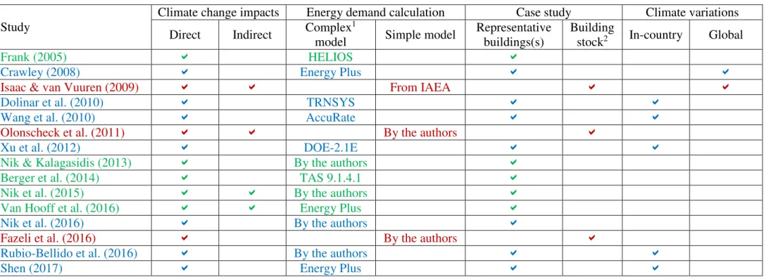
2.1 The direct and indirect impacts of climate change on building heat demand……...…...(11)
2.1.1 Representative building(s) simulation studies……….……….………...(12)
2.1.2 Representative building simulation studies with climate type variation…………...(14)
2.1.3 Large scale building stock simulation studies……….……..…..(17)
2.1.4 Comparison of the approaches previously used………...….……..(18)
2.2 Building energy demand models based on thermo-electrical analogy………...(21)
2.3 Representation of climate change impacts on building heat demand………..(25)
2.4 Preliminary conclusions from the literature survey……….……….……….……..(26)
CHAPTER 3: METHODOLOGY, PART I….……..………...(29)
3.1. Reference weather data………...……….…………...(29)
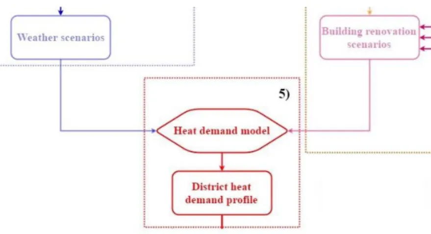
3.2 Weather scenarios……….………...(31)
3.3 Reference building data………...………..………...(32)
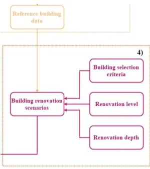
3.4 Building renovation scenarios……….………..………..(34)
vi
3.5.1 Model description………..……….………...(35)
3.5.2 Model validation………....…….………...(43)
3.5.2.1 Model results comparison with another energy demand software...…...(43)
3.5.2.2 Model results comparison with statistical building energy consumption data………...(45)
3.5.2.3 Model results comparison with on-site measured data.……....………..(46)
3.5.2.4 Elementary effect analysis of the developed model.…….…...………...(46)
3.6 Climate change impacts evaluation………...………...(49)
3.6.1 Heat demand related key performance indicators.…….………….……...…...(50)
3.6.2 District heating networks techno-economic indicators.…….………...(50)
CHAPTER 4: APPLICATION OF THE MODEL DEVELOPED WITHIN THE THESIS SCOPE………...(53)
4.1. Modelling the long-term impacts of climate change on district heat demand related parameters.…….………..………..(53)
4.1.1 Reference district state and weather data.…….………(54)
4.1.2 Weather and renovation scenarios.…….………..……..……...(58)
4.1.3 Results and discussion.…….………..………...(60)
4.1.4 Conclusions.…….………..………...(67)
4.2. Modelling the long-term impacts of climate change on district heating networks techno-economic parameters………..………(68)
4.2.1. Reference district state and weather data.………...…...(69)
4.2.2 Weather and renovation scenarios.………...….…………...…...(72)
4.2.3 Results and discussion.………..……….……...….………...(74)
4.2.4 Conclusions………...……….………...…...……….(78)
CHAPTER 5:THE EFFECT OF CLIMATE TYPE DIFFERENCES…………..…….(83)
5.1 Characteristic climate types definition……….…….………...(83)
5.2 Characteristic building case study selection………..………...(86)
5.3 Weather and building renovation scenarios………..………...(86)
5.4 Heat demand calculation and the results representation………...………...(88)
vii
5.6 Conclusions…………...………...(94)
CHAPTER 6: CONCLUSIONS, PART I ………..……...(97)
PART II: THE ENVIRONMENTAL PERFORMANCE OF DISTRICT HEATING NETWORKS………..(103)
CHAPTER 7: LITERATURE SURVEY, PART II………...……….(105)
7.1 Environmental performance assessment methods.……….………...…..(105)
7.2 The environmental performance district heating systems.…………...………….…….(107)
7.3 The environmental performance of building during its life-cycle.……...……….(112)
7.4. Preliminary conclusions from the literature survey.……….…...……….(117)
CHAPTER 8: METHODOLOGY (PART II)……...………....….……….(121)
8.1 The environmental performance of urban heating systems.………..……….(121)
8.1.1 Urban heating system outline and life-cycle phases definition.………….….(121)
8.1.2 Emergy flow of urban heating system construction phase.…………..……...(123)
8.1.2.1 Emergy flow of heat production unit construction.….……….……….(124)
8.1.2.2 Emergy flow of the network infrastructure placement.….……….…...(125)
8.1.2.3 Emergy flow of the building subsystem construction..………….……(129)
8.1.2.4 Emergy flow of human labour for system construction...…………...(130)
8.1.3 Emergy flow of urban heating system operation phase.………….…….(131)
8.2 The environmental performance of building during its life-cycle.……..…….……….(132)
8.2.1. Building system outline and life-cycle phases definition.………….…...….(133)
8.2.2 Resource allocation and building emergy flow calculation.….……….…….(135)
CHAPTER 9: APPLICATION OF THE METHODOLOGY DEVELOPED WITHIN THE THESIS PART II.……..……….………….….(141)
9.1 The environmental performance of urban heating systems.…………..………....(142)
9.1.1 District and system data.………..………..…….(142)
9.1.2 Results and discussion.………….……….……….………(149)
9.1.2.1 Urban heating systems construction phase.………..………(149)
9.1.2.2 Urban heating systems operation phase.……….…….……….(155)
viii
9.1.3 Conclusions.………..…….……….(160)
9.2 The environmental performance of urban heating systems within the urban environment………..(162)
9.2.1 Building data.……….………..…..….(163)
9.2.2 Results and discussion.……….…..……(165)
9.2.2.1 Building life-cycle without renovation phase.……….…...(165)
9.2.2.2 Building life-cycle with renovation phase.…………...………....(171)
9.2.3 Conclusions.…………..……….……….(177)
CHAPTER 10: CONCLUSIONS, PART II…...………..……...……….(181)
CHAPTER 11: CONCLUSION.…….………..………....(189)
11.1 Research motivation.………..……….……….(189)
11.2 Methodologies developed.………..……….……….(191)
11.3 Assessment of district heating potential in a context of climate change and building renovation………...……….….(192)
11.4 Concluding remarks and future work.……….…….(195)
APPENDIX A.………..……….……….(197)
A1: The list and the sources of the UEVs used.………..………….(199)
ix
LIST OF ABBREVIATIONS USED
ADP - Abiotic Depletion Potential; AP – Acidification Potential;
ASHRAE - American Society of Heating, Refrigerating and Air-Conditioning Engineers; BPIE - Building Performance Institute Europe;
CAPEX - Capital expenses; EP - Eutrophication Potential;
EPBD - Energy Performance of Buildings Directive; EPS – Expanded polystyrene
GIS – Geographical Information System; GPP – European Green Public Procurement; GWP – Global Warming Potential;
HTP – Human Toxicity Potential;
IAEA - International Atomic Energy Agency; IEA – International Energy Agency;
IGD - L’ Institut de la Gestion Déléguée;
INETI - Instituto Nacional de Engenharia, Technologia e Inovação; IOM - International Organization for Migration;
IPCC - Intergovernmental Panel on Climate Change; ISO – International Organization for Standardization; IWEC - International Weather for Energy Calculations; LCA - Life-cycle Assessment;
x
NZEB – Near Zero Energy Buildings; ODP - Ozone Layer Depletion; OPEX – Operating expenses;
POCP - Photo Oxidant Creation Potential; RD – Resource depletion;
xi
LIST OF FIGURES (numbered by chapter)
Figure 2.1 Building energy demand – outdoor air temperature function (temperature dependent
pattern);
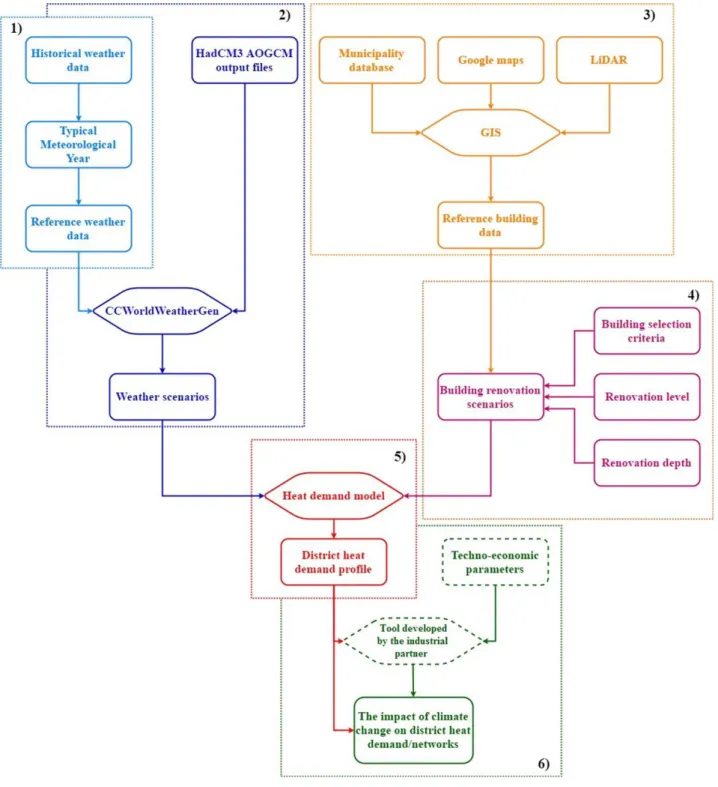
Figure 3.1 Outline of the methodology used in Part I of the thesis;
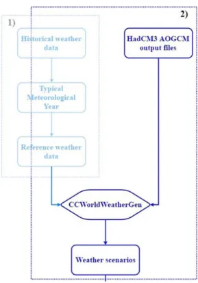
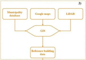
Figure 3.2 The methodology used for the reference weather data collection; Figure 3.3 The methodology used for the creation of future weather scenarios; Figure 3.4 The methodology used for reference building data collection;
Figure 3.5 The methodology used for the development of building renovation scenarios; Figure 3.6 Main heat demand model inputs and outputs;
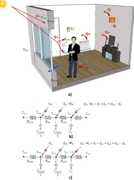
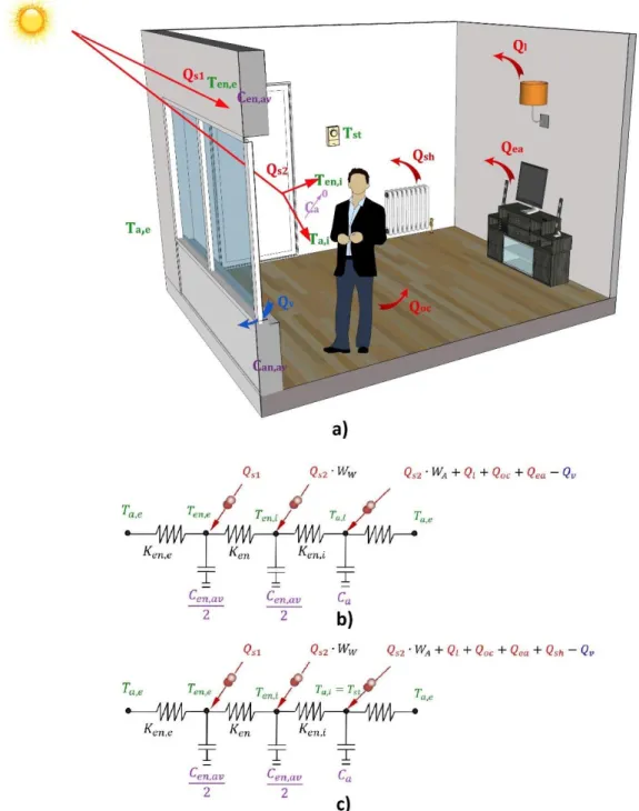
Figure 3.7 Physical representation of the model and the corresponding RC analogies ((a)
physical representation of the model, (b) RC model when the ambient temperature is higher or equal to the set point temperature, (c) RC model when ambient temperature is lower than the set point temperature);
Figure 3.8 Considered thermal bridges within the model; Figure 3.9 Selected buildings for model verification;
Figure 3.10 Climate change impacts evaluation methodology; Figure 4.1 Alvalade district overview;
Figure 4.2 Proposed sectioning of the Alvalade district;
Figure 4.3 The overview of heat demand slope coefficients for each building within the
Alvalade district;
Figure 4.4 The impact of climate change on district heat demand – outdoor air temperature
function slope and the number of heating hours;
Figure 4.5 The impact of climate change on district heat demand – outdoor air temperature
xii
Figure 4.6 The effects of direct and indirect impacts of climate change on district heat demand
density (for the district heating surface � =0.6 km2);
Figure 4.7 The specific annual heat demand distribution over the Alvalade district: reference
year and district state (a); low temperature scenario and shallow renovation path, year 2050 (b); High temperature scenario and deep renovation path (c);
Figure 4.8 Position of the St. Felix district in within the city of Nantes and the outline of the
residential building stock (data source: INSEE (2003) and Monteil (2010));
Figure 4.9 Overview of the building envelope renovation scenarios used in St. Felix case study
(renovation measures);
Figure 4.10 The impact of climate change on annual district heat demand and linear density; Figure 4.11 The impact of climate change on the heat production, sales and losses;
Figure 4.12 The impact of climate change on network production units and related CO2
emissions;
Figure 5.1 Locations selected for the case study;
Figure 5.2 The direct and indirect impact of climate change on heat demand-outdoor
temperature function parameters for selected locations ((a), (b), (c) – low, medium, high weather scenario (respectively));
Figure 5.3 The direct and indirect impact of climate change on heat demand for selected
locations, medium weather scenario and building renovation;
Figure 5.4 Load duration curves for Resolute (a) and Madrid (b), medium weather scenario and
building renovation;
Figure 5.5 The impact of climate type differences on heat demand decrease caused by the climate
change (medium weather scenario and building renovation): (a) Resolute, (b) Madrid;
Figure 8.1 Outline of the urban heating system; Figure 8.2 Urban heating system emergy diagram;
xiii
Figure 8.4 Building emergy diagram;
Figure 8.5 The impact of renovation measure on total building emergy flow over lifetime; Figure 9.1 Overview of the systems considered (figures are not in scale for clearer
representation);
Figure 9.2 Heat production units and energy sources considered for the studied systems; Figure 9.3 Emergy flow of the heat production unit construction (without human labor); Figure 9.4 Emergy flow of the network infrastructure construction (without human labor); Figure 9.5 Total construction phase emergy flow of the systems considered, with human labor
accounted;
Figure 9.6 The impact of network length on total emergy flow (construction and operation); Figure 9.7 The impact of total district heat demand on the UEV of heat delivered (construction
and operation);
Figure 9.8 Building used for the case study;
Figure 9.9 The impact of renovation measure on total building emergy flow over lifetime
(Scenario C);
Figure 9.10 The impact of building renovation timing on building UEV (reference value
� =3.30E+16sej/m2);
Figure 9.11 The impact of building renovation timing on EYR (reference value EYR=1.12); Figure 9.12 The impact of building renovation timing on EIR (reference value EIR=7.95); Figure 9.13 The impact of building renovation timing on ELR (reference value ELR= 8.13);
xv
LIST OF TABLES (numbered by chapter)
Table 2.1 Overview of the studies addressing the impact of climate change on building heat
demand;
Table 3.1 Outcomes of the model comparison
Table 3.2 Comparison of the RC model results and statistical building energy consumption data Table 3.3 Elementary effect analysis of the developed RC model;
Table 4.1 Glazing ratios obtained for the Alvalade district; Table 4.2 General parameters of the case study;
Table 4.3 Renovation depths;
Table 4.4 Assumed U-values for the renovation levels; Table 4.5 Glazing ratios for the district of St. Felix;
Table 4.6 Overview of the renovation scenarios used in St Felix case study (thermal properties
after renovation measures);
Table 4.7 Heat production costs for the regarded scenarios; Table 4.8 Results of a scenario with solar thermal collectors; Table 5.1 Climate types considered and characteristic locations; Table 5.2 Case study building parameters;
Table 5.3 Overview of the thermal properties within the building envelope renovation
scenarios;
Table 7.1 Overview of the studies on the environmental impacts of district heating systems; Table 7.2 Overview of the studies on the building environmental performance addressed within
the literature survey;
Table 9.1 Generic parameters required for the developed emergy evaluation; Table 9.2 Parameters of the boilers considered;
xvi
Table 9.3 Properties of the fuels combusted; Table 9.4 Overview of the scenarios considered;
Table 9.5 An overview of the calculated emergy flows for the regarded systems; Table 9.6 Emergy flows of infrastructure materials for the regarded network types; Table 9.7 Emergy flows of the building subsystem infrastructure materials;
Table 9.8 Calculated UEVs of heat delivered to the consumer for the studied systems
(construction and operation accounted);
Table 9.9 Emergy flow of substation materials;
Table 9.10 The impact of delivery distances on the total annual emergy flow of the systems; Table 9.11 Emergy flows of building construction phase;
Table 9.12 Emergy flows of building operation phase; Table 9.13 Emergy flows of building end-of-life phase; Table 9.14 Key performance indicators overview;
Table 9.15 The impact of different systems on building environmental performance;
Table 9.16 The impact of different heating systems on the shares of life—cycle phases in total
building emergy flow
Table 9.17 Building renovation phase emergy flows;
Table 9.18 Overview of major emergy flows for the regarded scenarios; Table 9.19 Sensitivity analysis (Scenario C);
xvii
NOMENCLATURE
Part I (in alphabetical order)
Item Unit Description
A [km2] Overall district surface;
A , [m2] Clear floor surface;
A , [m2] Surface of the clear roof;
A , [m2] Opaque walls surface (without glazing);
A , [m2] Total surface of the windows (glazing area);
A [m2] Total area of the element (including thermal bridges);
C [J/K] Average thermal capacity of the zone;
C [J/m2K] Specific heat capacity of the floors;
C [J/m2K] Specific heat capacity of the roof;
C [J/m2K] Specific heat capacity of the walls;
c [J/kgK] Specific air heat capacity;
c [J/kgK] Specific water heat capacity;
d [-] The elementary effect
f , [-] Fraction of the consumption profile for the regarded hour;
f , , [-] Working profile fraction of the h-th appliance;
f , [-] Occupancy profile fraction;
� [%] Building glazing ratio;
� [m] Zone height;
� , [W/m2] Global solar radiation for the regarded j-th hour;
� , [W/m2] Global solar radiation threshold value for lighting;
� � [W/K] Thermal conductance between the external envelope surface and
internal envelope surface; � , [W/K] Thermal conductance between the outdoor air and external surface of
the envelope; � , [W/K] Thermal conductance between the internal surface of the envelope and
internal ambient air;
� [W/K] Thermal conductance through the windows;
� [W/K] Thermal conductance through the window;
� [W/K] Thermal conductance through the floor;
� [W/K] Thermal conductance through the roof;
� [W/K] Thermal conductance through the walls;
� [m] Length of the regarded thermal bridge;
� [m] Length of the building corners;
� [m] Length of the floor thermal bridge;
� [m] Length of the parapet;
� [m] Length of the interfloor slabs;
� [m] Length of the windows thermal bridges;
� [m] Average length of one windows side;
n [corners] Number of corners per building;
n [oc.] Total number of occupants;
n [slabs] Number of interfloor slabs;
n [windows] Number of windows;
P [W/m2] Specific installed power of lighting equipment;
P [m] Zone perimeter;
P [m] Attached zone perimeter;
� [-] El. effect analysis selected levels in the space of the model input factors
xviii
Q [Wh/yr] Total district heat demand for the regarded period (year/heating season);
Q [W] District heat demand (in [W]);
Q [Wh/km2/yr] District heat demand density;
Q , , [Wh] Domestic hot water heating demand of i-th building for the j-th hour;
Q , [W] Hourly heat demand for the domestic hot water preparation;
Q , [W] Heat released from the h-th appliance;
Q , [W] Hourly heat release from the electric appliances;
Q [�] Heat gain from electrical appliances;
Q [�] Internal heat gains;
Q, [W] Hourly heat release from the lighting equipment;
Q [�] Heat gain from the lightning equipment;
Q , [W] Hourly heat release from the occupants;
Q [%] Heat gain from the occupants;
Q , , [Wh] Hourly heat space heating demand of i-th building for the j-th hour;
Q [�] Heat gains from the heating system;
Q [�] Solar heat gain on the external surface of the building envelope; Q [�] Solar heat gain on the internal surface of the building envelope; Q [�] Heat exchange due to the natural/mechanical ventilation; � [kg/oc./h] Domestic hot water demand per occupant for the regarded hour;
� , [W/oc.] Specific heat release from one occupant;
� , [vol./s] Level of air exchange in the zone;
� [m2] Floor surface area
� [m2] Roof surface area
� [m2] Wall surface area
� [m2] Window surface area
�, [K] Internal ambient air temperature;
� , [K] Temperature of water for domestic hot water preparation;
� [K] Temperature of the prepared domestic hot water;
� , [K] Temperature of the external envelope surface;
� , [K] Temperature of the internal envelope surface;
� [K] Internal set point (comfort) temperature;
� [°C] Outdoor air temperature (in [°C]);
� [W/m2K] Thermal transmittance of the clear element;
� [W/m2K] The mean U-value of the envelope
� [W/m2K] Clear floor thermal transmittance;
� [W/m2K] Thermal transmittance of the clear roof;
�, [W/m2K] Total thermal transmittance of the floor;
�, [W/m2K] Total thermal transmittance for the roofs;
�, [W/m2K] Total thermal transmittance of walls;
�, [W/m2K] Total thermal transmittance for windows;
� [W/m2K] Total thermal transmittance of the regarded envelope element;
� [W/m2K] Thermal transmittance of the clear wall (without glazing and thermal
bridges);
� [W/m2K] Thermal transmittance of clear windows;
� [m3] Zone volume;
�A [%] The fraction of solar radiation that penetrates through windows and
affects the internal ambient temperature; � [%] The fraction of total solar radiation that penetrates through windows and affects the internal wall temperature; α [W/°C] Heat demand –outdoor air temperature function slope coefficient; α [W/m2K] Heat convection coefficients on the external side of the floor;
xix
α [W/m2K] Heat convection coefficients on the external side of the walls;
α [W/m2K] Heat convection coefficients on the external side of the windows;
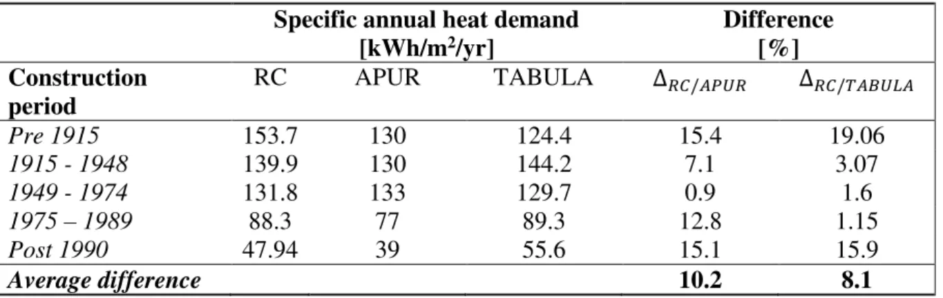
∆ [%] Percentage error for the annual heat demand;
∆ / [%] The difference between the RC model calculated results and
APUR/Tabula reports;
∆ [-] El. effect analysis step of parameter change
[%] The efficiency of the installed lighting equipment; [W] Heat demand –outdoor air temperature function intercept;
[-] Correction coefficient for incident beam;
[-] Correction coefficient to account for shading from the surrounding buildings; [-] Correction coefficient to account for the shading from the surrounding greenery; [-] Correction coefficient to account for building orientation; [-] Correction coefficient due to the windows blinds/shades;
μ [-] El. effect analysis mean value
μ , , [-] El. effect analysis modified mean value
ρ [kg/m3] Average air density;
σ [SD] Standard deviation between the heat demand hours;
σ [-] El. effect analysis deviation value
[W/K] The point thermal transmittance;
[W/mK] Linear thermal transmittance of the regarded heat bridge;
[W/mK] Linear thermal transmittance of the corner;
[W/mK] Linear thermal transmittance of the floor-to-ground transition; [W/mK] Linear thermal transmittance of the parapet heat bridge; [W/mK] Linear thermal transmittance of the interfloor slab; [W/mK] Linear thermal transmittance of the window-to-wall thermal bridge; Ω [-] El. effect analysis Region of experimentation of the model inputs
Part II (in alphabetical order)
Item Unit Description
a [-] Ground albedo;
A [m2] Total useful building floor surface;
A [m2] Construction site surface (footprint);
C , [kg] Additional elements delivery vehicle transportation
maximum capacity; C , [kg] Maximum capacity of the vehicle used for the delivery
of an additional material for network infrastructure placement; C , [kg] Building subsystem elements transportation vehicle
maximum capacity;
C , [kg] Excess ground transportation vehicle maximum
capacity;
C , [kg] Fuel delivery vehicle maximum capacity;
C , [kg] Heat production unit material transportation vehicle
maximum capacity; C , [rolls] Pipe transportation vehicle maximum rolls capacity;
C , [pipes] Maximum segment capacity of pipe transportation
vehicle; D , [km] Building subsystem elements transportation distance
xx
D [km] Daily distance crossed by one employee;
D [km] Daily distance crossed by one employee;
D , [km] Transportation distance during one delivery of
materials for heat production unit construction; D , [km] Transportation distance per one delivery of additional
elements; D , [km] Transportation distance for delivering an additional
material used for network infrastructure placement;
D , [km] Excess ground transportation distance per one
delivery; D , [km] Transportation distance per one delivery of pipes;
D , [km] The delivery distance crossed by the fuel delivery
vehicle per each fuel delivery;
d , [m] Diameter of the g-th pipe type placed;
d [m] Network trench depth;
E , [sej] Emergy flow of materials and resources used for the
building subsystem elements;
E , [sej] Emergy flow of building subsystem materials and
resources used for the building subsystem elements installation;
E , [sej] Emergy flow of building subsystem elements
transportation;
E , [sej] Building subsystem construction emergy flow;
E , [sej] Building subsystem emergy flow;
E , [sej] Emergy flow of human labor required for the
construction of each system component and final assembly;
E , [sej] Heat production unit construction emergy flow;
E, [sej] Network infrastructure placement emergy flow;
E, [sej] System construction emergy flow;
E , [sej/emp/yr] Individual emergy flows of employees with college
education;
E [sej] Emergy flow of heavy construction machines;
E [sej] Emergy flow of construction workers daily
commuting; E [sej] Emergy flow of fuel used for on-site electricity generators; E , [sej] Emergy flow of electricity consumed from the grid;
E , [sej] Emergy flow of end-of-life phase without building
renovation;
E , [sej] Emergy flow of end-of-life phase after building
renovation; E, [sej/yr] Emergy flow of the e-th fuel type combusted;
E [sej/yr] Emergy flow of heat used for heating the premises during the building lifetime;
E , [sej] Emergy flow of heat production unit material
transportation; E [sej] Heat production unit materials and assembly emergy flow; E , [sej/emp/yr] Individual emergy flows of employees with high
school education; E , [sej] Emergy flow of transportation for each j-th material;
E , [sej] Additional elements emergy flow;
E , [sej] Emergy flow of network infrastructure additional
xxi
E , [sej] Emergy flow of network infrastructure additional
elements transportation; E , [sej] Emergy flow of additional material used for network
infrastructure placement;
E , [sej] Additional material transportation emergy flow;
E , [sej] Excess ground transportation emergy flow;
E , [sej] Emergy flow of the pipes used;
E , [sej] Pipe laying process emergy flow;
E , [sej] Emergy flow of pipe laying process with heavy
machines;
E , [sej] Pipe materials emergy flow;
E , [sej] Pipe transportation emergy flow;
E , [sej] Trench excavation emergy flow;
E , [sej/yr] Emergy flow of employees home-to-work daily
commuting; E , [sej/yr] Emergy flow of resources used for heat generation;
E , [sej/yr] Emergy flow of heat generation resources
transportation; E , [sej/yr] Emergy flow of human labor required to operate the
system;
E , [sej] Emergy flow of human labor used during the
construction/renovation phase;
E , [sej/yr] Annual emergy flow of system operation;
E , [sej/J] Emergy flow of the operation phase over the total
system lifetime;
E , [sej] Building operation emergy flow for a reference
building state; E , [sej] Emergy flow of building operation within its reference
state;
E [sej] Emergy flow of building renovation;
E , [sej] Soil erosion emergy flow;
E [sej] Emergy flow of solar radiation on a building
construction site; E [sej/yr] Emergy flow of annual solar gains on the building envelope;
E , [sej] Emergy flow of i-th subsystem construction;
E, [sej] Total building emergy flow without renovation phase;
E, [sej] Total building emergy flow with renovation phase;
E , [sej] Emergy flow of water consumed during the building
construction phase; E , [sej] Emergy flow of water consumed during the building
lifetime;
EIR [sej] Emergy investment ratio;
ELR [sej] Emergy loading ratio;
EYR [sej] Emergy yield ratio;
e [J/kg] Soil energy content;
F [sej] Purchased resources consumed by the system;
�C , [l/km] Additional elements delivery vehicle fuel consumption
with full load; �C , [l/km] Additional elements delivery vehicle fuel consumption
without a load; �C , [l/km] Fuel consumption with full load of the vehicle used
for transporting an additional material for network infrastructure placement;
xxii
�C , [l/km] Fuel consumption without a load of the vehicle used
for transporting an additional material for network infrastructure placement; �C , [l/km], Building subsystem elements transportation vehicle
fuel consumptions with full load; �C , [l/km], Building subsystem elements transportation vehicle
fuel consumption without a load; �C , [l/km] Average fuel consumption of the passenger cars used
by the employees for home-to-work commuting;
�C , [l/km] Passenger car average fuel consumption;
�C , [l/h] Hourly fuel consumption of the machine considered
with a full load; �C , [l/h] Hourly fuel consumption of the machine without a
load; �C , [l/km] Excess ground transportation vehicle fuel consumption
with full load; �C , [l/km] Excess ground transportation vehicle fuel consumption
without a load; �C , [l/h] Trench excavation machine hourly fuel consumption
with full load; �C , [l/h] Trench excavation machine hourly fuel consumption
without a load; �C , [l/km] Fuel delivery vehicle fuel consumption with full load;
�C , [l/km] Fuel delivery vehicle fuel consumption without a load;
�C , [l/km] Heat production unit material transportation vehicle
fuel consumption with full load; �C , [l/km] Heat production unit material transportation vehicle
fuel consumption without a load; �C , [l/km] Pipe transportation vehicle fuel consumption with full
load; �C , [l/km] Pipe transportation vehicle fuel consumption without a
load;
f [%] The amount of organic substance in soil;
H [MJ/yr] Annual heat demand;
H [J] Total heat demand (with losses accounted) ;
� , [h] Number of operating hours for the machine
considered;
� [h] Number of hours for excavation required by an
adequate machine;
� [m] Pipe infrastructure height;
� [h] Time required for excavating machine to make one
complete excavating move; � , [J/m2/yr] Annual amount of solar radiation for the studied
location;
�H� [J/l] Diesel fuel low heating value;
�H� [MJ/kg] [MJ/m3] Regarded fuel low heating value;
� [m] Pipe infrastructure length;
� [m] Network length;
� [m] Length of a pipe in one roll;
� [m] Length of one pipe segment;
� [m] Network trench length;
� , [kg] Mass of the materials used for s-th additional element;
� , [kg] The amount of sand and gravel mixture used to cover
xxiii
� , [kg] The amount of x-th material used during network
infrastructure placement; � , [kg] The amount of the v-th material used for building
subsystem elements installation; � , [kg] The amount of i-th type of material used for heat
production unit construction; �, [kg] The amount of j-th material used during the subsystem
construction (of total n materials);
� , [kg] The amount of excess ground material to be
transported to the landfill;
� , [kg/m] The specific mass of concrete used for network
covering;
� , [kg/m] The specific mass of pavement used for trench
covering; N [sej] Indigenous non-renewable resources consumed by the system; �D , [del.] Number of deliveries for building subsystem elements
transportation; �D , [del.] The number of material deliveries for heat production
units construction; �D , [del.] Number of deliveries for the additional elements
transportation; �D , [del.] Number of deliveries for an additional material used
for network infrastructure placement; �D , [del.] Number of excess ground transportation deliveries;
�D , [del.] Number of pipe deliveries;
�D , [del.] Number of deliveries for fuel transportation;
n [days] Number of days required for the system construction and assembly;
n [days] Number of days required to complete building
construction;
n , [h] Number of hours worked daily by one employee;
n , [emp.] The number of employees with college education
engaged in the j-th process; n [emp.] Number of employees used for system construction;
n [c.w.] Number of engaged construction workers;
n , [mov.] Number of excavating moves made by machine;
n [h/day/emp.] Number of hours per day worked by one construction worker; n , [emp.] The number of employees with high school education
engaged in the j-th process;
n [yr] Expected system lifetime;
n [oc.] Number of occupants;
n [days] Number of working days;
n , [h/day/emp.] Hours per day worked by one employee;
n [emp.] Number of employees required for system operation;
n [rolls] Number of required pipe rolls;
n [segments] Number of pipe segments;
Q [J/yr] The amount of heat consumed annually during the heating season; Q [J/yr] Annual solar gains on the building envelope during the heating season; � , [J] The amount of an additional w-th energy resource used
xxiv
� , [J] The amount of an additional w-th energy resource used
for building subsystem elements installation;
�, [kg][m3] The amount of each fuel type combusted;
� , [J] The amount of j-th additional energy resource used for
the heat production unit assembly;
R [sej] Indigenous renewable resources consumed by the
system;
� [K] Heat sink temp. for Carnot efficiency calc.
� [K] Heat source temp. for Carnot efficiency calc.
� [yr] Time required for building construction;
� , [yr] Time of building operation within the reference state;
� , [yr] Period of building operation within its reference state;
� [yr] Total time of building operation;
� , [sej/kg] UEV of the s-th material used for s-th additional
element; � , [sej/J] UEV of an additional w-th energy resource used for an
additional element assembly;
� , [sej/kg] UEV of the x-th material used;
� [sej/m2] Building UEV;
� , [sej/kg] UEV of the v-th material used for building subsystem
element installation; � , [sej/J] UEV of the w-th energy resource used for building
subsystem elements installation; � , [sej/h] UEV of human labor used for system construction;
� , [sej/h] UEV of human labor of construction workers;
� [sej/J] Diesel fuel UEV;
� , [sej/J] The UEV value of i-th electricity production source;
� [sej/J] UEV of the electricity produced for the case study location;
�, [sej/kg] [sej/m3] UEV of each fuel type combusted;
� [sej/J] UEV of heat delivered;
� [sej/J] UEV of the heat delivered to the consumer;
� , [sej/h] The UEV of human labor for each j-th process;
� , [sej/kg] UEV of the i-th heat production unit material;
� , [sej/J] UEV of j-th additional energy resource used for the
assembly;
�, [sej/kg] UEV of the regarded material;
� [sej/J] Land use UEV;
� , [sej/h] UEV of human labor for network operation;
� [sej/J] Solar energy UEV;
� [sej/kg] Water UEV;
� [m3] Excavating machine the bucket volume;
� [m3] Volume of the soil excavated;
� [m3] The amount of excavated soil used for trench refilling;
� [m3] Volume of the pipe infrastructure placed in the
excavated trench;
� [m3] Volume of the trench to be excavated;
� [m3] Volume of the water used during the building
construction phase;
� [J/yr] Annual electricity consumption;
� [m] Pipe infrastructure width;
� [m] Network trench width;
α [%] The share of soil in the mixture for network trench filling;
xxv
[%] Fuel share in annual heat production;
Additional elements delivery vehicle fuel consumption ratio; [-] Fuel consumption ratio of the vehicle used for transporting an additional material for network infrastructure placement; [-] Building subsystem elements transportation vehicle fuel consumption ratio; [-] Fuel consumption ratio of the machine considered; [-] Excess ground transportation vehicle fuel consumption
fuel consumption ratio; [-] Trench excavation machine fuel consumption ratio; [-] Fuel delivery vehicle fuel consumption ratio; [-] Heat production unit material transportation vehicle fuel consumption ratio; [-] Pipe transportation vehicle fuel consumption ratio; ∆ [sej] Emergy saving achieved by renovation measures;
, [%] The regarded i-th electricity production source share
in total electricity production;
[%] Carnot efficiency of the system;
[%] Heat production unit energy transformation efficiency;
[%] Network efficiency;
[l/m2] Generator fuel consumed to produce the required
amount of electricity on construction site during the construction phase;
ρ [kg/m3] Excavated soil average density;
ρ [kg/m3] Average soil density;
ρ [kg/m3] Average density of sand and gravel mixture;
ρ [kg/m3] Water density;
xxvii
PERSONAL REFERENCES Journal publications
Andrić, I., Jamali-Zghal, N., Santarelli, M., Lacarrière, B., Le Corre, O., 2015. Environmental performance assessment of retrofitting existing coal fired power plants to co-firing with biomass: carbon footprint and emergy approach. Journal of Cleaner Production, 103, pp13-27. DOI: https://doi.org/10.1016/j.jclepro.2014.08.019;
Andrić, I., Gomes, N., Pina, A., Ferrão, P., Fournier, J., Lacarrière, B., Le Corre, O., 2016. Modelling the long-term effect of climate change on building heat demand: case study on a district level. Energy and Buildings, 126, pp77-93. DOI:
https://doi.org/10.1016/j.enbuild.2016.04.082;
Andrić, I., Pina, A., Ferrão, P., Lacarrière, B., Le Corre, O., 2017. Environmental performance of district heating systems in urban environment: an emergy approach. Journal of Cleaner
Production, 142 (1), pp. 109-120. DOI: https://doi.org/10.1016/j.jclepro.2016.05.124;
Andrić, I., Pina, A., Ferrão, P., Lacarrière, B., Le Corre, O., 2016. Assessing the feasibility of using the heat demand-outdoor temperature function for a long-term district heat demand forecast. Elsevier Energy Procedia, 116©, p462/471. ISSN: 1876-6102;
Andrić, I., Pina, A., Ferrão, P., Lacarrière, B., Le Corre, O., 2017. The impact of climate change on building heat demand in different climate types, Energy and Buildings, 149, p225-234. DOI:
https://doi.org/10.1016/j.enbuild.2017.05.047;
Andrić, I., Pina, A., Ferrão, P., Lacarrière, B., Le Corre, O., 2017. The impact of renovation measures on building lifecycle: an emergy approach. Journal of Cleaner Production, 162, p776-790. DOI: https://doi.org/10.1016/j.jclepro.2017.06.053;
Conferences
Andrić, I., Darakdjian, Q., Ferrão, P., Fournier, J., Lacarrière, B., Le Corre, O., 2014. The impact of global warming on district heating demand: The case of St Félix. 14th International
Symposium on District Heating and Cooling, Stockholm, Sweden, 7-10th September 2014;
Andrić, I., Pina, A., Silva, C., Ferrão, P., Fournier, J., Lacarrière, B., Le Corre, O. The impact of climate change and building renovation on heating related CO2 emissions on a neighborhood
xxviii
Andrić, I., Pina, A., Ferrão, P., Lacarrière, B., Le Corre, O., 2016. Assessing the feasibility of using the heat demand-outdoor temperature function for a long-term district heat demand forecast. 15th International Symposium on District Heating and Cooling, Seoul, South Korea,
4th -7th September 2016;
Andrić, I., 2016. Time management for entrepreneurs, 5th Annual Inno Energy Scientist
Conference, Barcelona, 16-18th of November 2016;
Andrić, I., Pina, A., Ferrão, P., Fournier, J., Lacarrière, B., Le Corre, O., 2017. The impact of climate change on the techno-economical parameters of district heating networks. 3rd
International Conference on Smart Energy Systems and 4th Generation District Heating,
Copenhagen, Denmark, 11-12th September 2017;
AWARDS AND ACHIEVEMENTS
1st Pitching prize, 4th Annual Inno Energy Scientist Conference, Berlin, Germany, 20th – 20nd October 2015;
1st Pitching prize, 4th International DHC+ Summer School, Warsaw, Poland, 21st – 27th August 2016;
3rd prize, Iberdrola Energy Challenge 2017, Madrid, Spain, 31st January – 10th July 2017;
Best Pitch Prize, Energy Solutions Design for Eco-Districts, Grenoble, 3rd-7th July 2017; End User’s Prize, Energy Solutions Design for Eco-Districts, Grenoble, 3rd-7th July 2017;
xxix
EXTENDED ABSTRACT/ RÉSUMÉ ÉTENDU (in French/en français)
Le changement climatique est un phénomène sans équivoque, établi sur la base des températures observées dans les couches de l’atmosphère et dans les océans, la superficie des surfaces enneigées et sur la fonte des glaces induisant une augmentation du niveau moyen des océans. Différents rapports d’institutions internationales recherchant les causes, les potentiels impacts et les conséquences de ce changement climatique suggèrent qu’il est extrêmement
probable que l’augmentation de gaz à effet de serre dans l’atmosphère, dégagés par l’activité
anthropique, est l’un des principaux facteurs de ce changement climatique. Comme le chauffage de l’immobilier est l’un des secteurs émettant le plus de gaz à effet de serre, et que ce secteur est, de surcroît, en constante progression (en lien avec l’augmentation de la population), la réduction de cette consommation d’énergie et de ces émissions afférentes de gaz à effet de serre pourrait contribuer significativement à limiter le changement climatique.
Les réseaux de chaleur sont communément proposés dans la littérature comme une solution technique pertinente d’un point de vue environnementale pour fournir les besoins de chauffage dans les logements, les magasins et les entreprises. Ces réseaux ont de multiples intérêts, tels que : une production centralisée pouvant être hors du cœur des centres villes, une large gamme d’utilisation d’énergie renouvelable et/ou de déchets, et une amélioration du confort et de la sécurité de la chaleur fournie. Par conséquent, le développement des réseaux existants ainsi que la construction de nouveaux réseaux sont bien documentés, y compris dans les rapports stratégiques officiels de l’Union Européenne (EU) traitant de la « décarbonisation » des systèmes énergétiques dans l’UE. Cependant, la construction de tels réseaux nécessite des investissements financiers conséquents, amortis par la vente de chaleur sur des longs temps de retour. Toute réduction de consommation d’énergie d’un tel réseau impacterait sa rentabilité (ou même sa faisabilité).
Ces réductions de consommation peuvent être qualifiées de directes ou indirectes, par rapport au phénomène du changement climatique. D’une part, la différence entre la température interne d’un bâtiment (celle de confort pour les occupants) et son environnement (augmentation future de la température extérieure) devrait se réduire, limitant la quantité de chaleur à fournir, notamment celle des clients connectés à un réseau de chaleur. Cet aspect peut être classé comme un impact direct du changement climatique sur la demande de chaleur des bâtiments. D’autre part, les politiques incitant à la sobriété énergétique dans le secteur du bâtiment (comme la directive de performance énergétique des bâtiments ou la directive 2010/31/EU) ont été (ou sont en cours d’être) transcrites dans les textes officiels nationaux afin d’encourager la
xxx
rénovation dans ce secteur partout en Europe. L’amélioration des performances de l’enveloppe d’un bâtiment rénové induit une diminution de la consommation d’énergie pour son chauffage. Cet aspect peut être classé comme un impact indirect du changement climatique.
Cependant, l’évaluation de la performance énergétique d’un système, quel qu’il soit, considérée sur la seule base de ces émissions pendant sa phase opérationnelle pourrait amener à des résultats erronés : les impacts environnementaux associés pendant la phase de construction sont fréquemment pris en compte. Plus précisément, cette évaluation est d’autant plus importante pour les réseaux de chaleur urbains que ces réseaux sont composés d’éléments (unité centralisée de production de grande capacité, réseau de distribution avec des tuyaux de grands diamètres et connections aux bâtiments au niveau des sous-stations ou de systèmes assimilés) à fort impact environnemental (tel que l’acier etc…). Par conséquent, l’impact de toutes les ressources consommées, directement ou indirectement, pendant toute la durée de vie d’un système (comme un réseau de chaleur) doit être pris en considération afin d’avoir une évaluation adéquate de la performance de ces-dits systèmes. En outre, afin de caractériser la performance environnementale d’un réseau urbain de chaleur dans son environnement, cette performance doit être comparée à celle d’une solution de référence fournissant le même besoin de chaleur. De plus, cette caractérisation doit être effectuée en tenant compte de la manière dont la chaleur consommée par les bâtiments connectés au réseau de chaleur affecte la performance environnementale du bâtiment lui-même (i.e. changement de perspective de l’analyse environnementale, du propriétaire du réseau de chaleur à celui du bâtiment).
Le champ de recherche de cette thèse peut être scindé suivant deux approches principales: L’évaluation de l’impact du changement climatique sur les réseaux urbains de chaleur,
en tenant compte des aspects direct et indirect, décrits précédemment.
L’évaluation de la performance environnementale des réseaux urbains de chaleur dans son environnement, en tenant compte de toutes les ressources consommées sur la durée de vie du système (et de ses équipements), de la phase amont de la construction à sa phase de fonctionnement.
xxxi
Figure : Modèle thermoélectrique pour l’estimation du besoin de chaleur d’une enveloppe
à température intérieure contrôlée;
Pour évaluer les impacts (direct et indirect) du changement climatique sur les réseaux urbains de chauffage, un modèle basé sur une analogie thermoélectrique de l’enveloppe d’un bâtiment (voir figure ci-dessus) a été créé et comparé à d’autres logiciels ou méthodes (CCWorldWetaherGen, ArcGIS, LiDAR). La méthodologie ainsi proposée permet d’évaluer les impacts directs du changement climatique. Le modèle thermoélectrique de demande de chaleur d’un bâtiment a été comparé d’une part avec le logiciel Design Builder v4.6 (Energy Plus v.8.3), logiciel de référence dans la simulation de la demande énergétique d’un bâtiment, et d’autre part avec des données statistiques de demande de chauffage provenant de rapports nationaux d’institutions gouvernementales des pays étudiés. Les résultats des validations de la
xxxii
demande annuelle de chauffage sont satisfaisants : d’une part, la différence entre le modèle thermoélectrique et le logiciel Energy Plus est en moyenne de 4.5 %, d’autre part, la différence entre le modèle thermoélectrique et les données statistiques (comportant le type de bâtiment et sa période de construction) issues de rapports d’agence nationale est entre 8 % à 10 %. Dans ces validations, la marge d’erreurs est faible et est inférieure à la limite maximale communément reportée dans la littérature (20 %), pour les modèles simplifiés de demande de chauffage. Après cette validation, la méthodologie a été appliquée à deux cas : à un quartier de Lisbon (Portugal), nommé Alvalade se composant de 655 bâtiments, et à un quartier de Nantes (France) nommé St. Félix se composant de 622 bâtiments. Pour ces 2 cas, de multiples scénarii ont été considérés, i.e. des données météorologiques venant de modèles du GIEC (Groupe International d’Expert du Climat) et de rénovation (programmation et « intensité » de rénovation). Pour compléter ces résultats, une étude spécifique consistant à imaginer un même bâtiment construit à 5 endroits du globe a été menée. La finalité de cette étude est de voir si les conclusions des 2 cas précédents sont généralisables.
Pour évaluer la performance environnementale d’un réseau urbain de chauffage dans son environnement, l’approche méthodologique de l’empreinte énergétique (appelée eMergie dans la littérature) a été considérée dans cette thèse. Dans cette partie, les premiers travaux de cette thèse s’intéressent plus particulièrement à la performance environnementale de la production-distribution des réseaux de chauffage urbains, en tenant compte des ressources amont et aval consommées pendant la durée de vie d’un réseau : construction, fonctionnement (la phase de démolition n’a pas été considérée car il n’existe pas de cas de démolition d’un réseau, même après plusieurs décades de fonctionnement – selon la bibliographie consultée et la connaissance approfondie de l’auteur). La méthodologie développée peut être appliqué à un réseau urbain de chauffage quelconque : les applications dans cette thèse considèrent différents modes de production de chaleur. Dans cette partie, les secondes analyses environnementales de cette thèse s’intéressent plus particulièrement au consommateur final dans le bâtiment. L’analyse tient compte, comme précédemment, de la phase de construction, de fonctionnement du bâtiment mais aussi la phase de démolition ainsi que la phase de rénovation éventuelle. La méthodologie développée peut être appliquée à un bâtiment quelconque, indépendamment de sa période de construction, à condition que les données d’entrée soient disponibles. Cette méthodologie a été d’abord appliquée pour comparer 2 types de réseaux de chaleur : un réseau moderne à 4 tuyaux ESPEX et un réseau traditionnel à 2 tuyaux. Les moyens centralisés associés à la production ont été comparés à une production décentralisée et individuelle utilisant du gaz naturel de ville. Ces différentes configurations ont été appliquées sur un quartier de Värnamo (Suède), nommé Vråen. Afin d’évaluer dans quelle mesure la chaleur consommée par
xxxiii
ce quartier peut impacter la performance environnementale, la méthodologie a aussi été mise en œuvre sur un immeuble d’habitation situé dans la ville de Šabac (Serbie).
A partir des résultats obtenus de ces études de cas, il est possible de conclure que les réseaux urbains de chaleur pourraient avoir un grand potentiel pour atteindre les objectifs « soutenables » des politiques de l’UE, si et seulement si les aspects suivants sont pris en considération dès la phase de conception :
Production de chaleur à partir de ressources renouvelables ;
Utilisation de réseaux urbains modernes, avec une infrastructure compacte, utilisant des matériaux ayant un impact environnemental faible;
Capacités de production conçues pour une potentielle baisse de la demande de chaleur due à l’impact direct ou indirect du changement climatique (par exemple, installation de 2 chaudières en base, d’une capacité cumulée égale à celle d’une grande chaudière);
Utilisation de combustibles les moins nuisibles à l’environnement pendant les périodes de pointe;
Prise en compte de l’effet du changement climatique selon les régions sur la demande de chaleur;
Développement de plans de financement alternatif afin d’éviter l’augmentation des prix du kilowatt-heure chaleur ayant pour conséquence éventuelle la déconnection de clients.
Des pistes de travaux supplémentaires peuvent être suggérées:
validation du modèle thermoélectrique sur des mesures sur site ; développement d’une partie climatisation dans le modèle ;
développement d’une communication avec d’autres logiciels commerciaux, afin d’intégrer les impacts du changement climatique sur la « soutenabilité » de l’environnement urbain, et plus particulièrement de ses réseaux de chaleur et de froid.
1
3
CHAPTER 1: INTRODUCTION
1.1 Research motivation
C0limate change is unequivocal, as proved by the observed global air and ocean temperature 00es, widespread snow and ice melting and the rise in average sea level (IPCC, 2014). Human influence on the climate system is clear – anthropogenic greenhouse gas emissions have significantly increased since the dawn of the industrial era due to the rapid economic and population growth. Consequently, these emission patterns have led to currently all-time high atmospheric concentrations of greenhouse gases. The effects have been detected throughout the whole climate system. The summary of recent scientific reports suggests that it is extremely likely that increased concentration of greenhouse gases and previously mentioned anthropogenic drivers have been the dominant cause of observed warming (IPCC, 2014). Additionally, there is a high probability that heat waves will occur more often and have a longer duration in the future. Climate change already has a widespread impact on human and natural systems, and the continuous emission of greenhouse gasses would cause further warming and long-term changes in all components of Earth’s climate system. In the summary report by the IPCC (Intergovernmental Panel on Climate Change), it was concluded that cumulative emissions of CO2 in all scenarioswould significantly determine global mean surface warming
by the late 21st century and beyond (IPCC, 2014). These long term changes would increase the
possibility of severe and irreversible impacts for global society and ecosystems. Thus, substantial emissions reductions in the decades to come could limit climate change risks, foster the effective adaptation measures, reduce the climate change mitigation costs and contribute to environmental pathways for sustainable future.
According to the Climate Analysis Indicators Tool (World Resources Institute, 2016), 64.5% of global anthropogenic greenhouse gas emissions comes from the energy sector. Worldwide, about 18% of total energy end-use is consumed in the building residential sector (U.S. Energy Information Administration, 2013). However, in developed countries, this sector is the main source of CO2 emissions. For example, in the U.S.A., about 44.5% of total CO2
emissions originate from this sector, which is significantly more than the industrial and transportation sectors (21.1 % and 30.7 %, respectively (Architecture 2030, 2015)). Considering the constant increase in built environment due to population increase (predicted to reach 10 billion in 2056 (United Nations, 2015)), migrations from rural to urban areas (current
4
urban population of 3.9 billion is estimated to grow to 6.4 billion by 2050 (IOM, 2015)) and increase in global gross domestic product per capita, the reduction of energy consumption and related greenhouse gas emissions from the building sector in the future presents a challenging task.
Theoretically, buildings consume different forms of energy in order to provide specific services, and maintain their performance constant in time with respect to various variable conditions, such as climate (Pulselli et al. 2007). Considering that the activity most responsible for energy consumed in buildings is typically maintaining comfort conditions (especially heating in the countries with continental climate – for example 32 % in U.S.A, (U.S. Department for Energy, 2008)), enabling sustainable heating systems for the increasing urban environment could significantly contribute to proposed global climate change mitigation measures.
District heating systems are commonly proposed in the literature as an environmentally friendly solution for providing heating services for the built environment due to their benefits, such as centralized heat production located outside city centers, large scale utilization of renewable heat sources (solar, geothermal etc.) and waste heat, overall environmental and economic efficiency, comfort and the security of supply for the consumers. In 2014, there was about 6000 district heating systems operating in Europe with an overall distribution network length of 200,000 km (Connolly et al., 2014). Considering the scarcity of these systems in Europe (for example, in Scandinavian countries district heating systems cover up to 40-60 % of total heat demand (Swedish Energy Agency, 2012) while in France this share is only 5 % (IGD, 2009)), the expansion of such systems is already suggested in the literature. The subject has been widely researched in several scientific reports, such as “Heat Roadmap Europe 2050” (Connolly et al., 2012), “Decarbonizing heat in buildings 2030-2050” (IAEA, 2012), and “Towards decarbonizing heat: maximizing the opportunities for Scotland” (The Scottish Government, 2012). Additionally, in the report on an EU Strategy on Heating and Cooling (European Parliament, 2016), it was stated that “more must be done in order to switch
remaining (heat) demands away from burning imported fossil fuels in individual boilers towards sustainable heating and cooling options”. Connolly et al. (2014) explored the benefits
of combining district heating with heat savings to decarbonize the EU energy system. The conclusions were that district heating should be considered an essential cost-effective technology for the EU energy system decarbonization. As a successful example, energy transition in Sweden by using low-carbon district heating within the 1950 – 2014 period was thoroughly described in the paper of Di Lucia & Ericsson, (2014). Moreover, Lake et al. (2017)