Titre:
Title:
Linear model predictive control for the reduction of auxiliary electric
heating in residential self-assisted ground-source heat pump
systems
Auteurs:
Authors
: Massimo Cimmino et Alex Laferrière
Date: 2019
Type:
Article de revue / Journal articleRéférence:
Citation
:
Cimmino, M. & Laferrière, A. (2019). Linear model predictive control for the reduction of auxiliary electric heating in residential self-assisted ground-source heat pump systems. Science and Technology for the Built Environment, 25(8), p. 1095-1110. doi:10.1080/23744731.2019.1620564
Document en libre accès dans PolyPublie
Open Access document in PolyPublieURL de PolyPublie:
PolyPublie URL: https://publications.polymtl.ca/5504/
Version: Version finale avant publication / Accepted versionRévisé par les pairs / Refereed Conditions d’utilisation:
Terms of Use: Tous droits réservés / All rights reserved
Document publié chez l’éditeur officiel
Document issued by the official publisher Titre de la revue:
Journal Title: Science and Technology for the Built Environment (vol. 25, no 8)
Maison d’édition:
Publisher: Taylor & Francis
URL officiel:
Official URL: https://doi.org/10.1080/23744731.2019.1620564
Mention légale:
Legal notice:
This is an Accepted Manuscript of an article published by Taylor & Francis in Science and Technology for the Built Environment on 25 June 2019, available online: http://www.tandfonline.com/10.1080/23744731.2019.1620564.
Ce fichier a été téléchargé à partir de PolyPublie, le dépôt institutionnel de Polytechnique Montréal
This file has been downloaded from PolyPublie, the institutional repository of Polytechnique Montréal
Alex Laferrière is a Master’s student. Massimo Cimmino is an assistant professor.
*Corresponding author e-mail: alex.laferriere@polymtl.ca
Linear model predictive control for the reduction of auxiliary
electric heating in residential self-assisted ground-source heat
pump systems
ALEX LAFERRIÈRE
1, MASSIMO CIMMINO
11Department of Mechanical Engineering, Polytechnique Montréal, Montreal, Quebec, Canada
This paper presents a linear model predictive control strategy for the operation of a “self-assisted” ground-source heat pump (GSHP) to reduce auxiliary electric heating in residential applications equipped with undersized boreholes. The self-assisted configuration uses an electric heating element at the heat pump outlet to inject heat into the bore field when approaching peak power demand. A linear control-oriented model is proposed to account for both the source-side and load-side GSHP dynamics. The ground heat transfer is predicted using the bore field’s ground-to-fluid thermal response factor, thus allowing for any bore field configuration while accounting for thermal capacity effects. Real historic ambient temperature forecasts and their corresponding historic recorded ambient temperatures from Montreal are used in this paper. The COP non-linearity is circumvented with an iterative approach. A Kalman filter is used to dynamically adjust the bias on the predicted returning fluid temperature. On a borehole undersized by 15%, the control strategy reduces auxiliary electric heating by 96% over 20 years at the cost of a 5.53% increase in total energy consumption. Due to the occasional simultaneous heat injection and auxiliary heating, the yearly peak power demand is increased.
Introduction
Ground-source heat pumps (GSHP), coupled to vertical geothermal boreholes, are an energy-efficient method to meet the heating and cooling loads of buildings. In cold climates, GSHPs will gradually exhaust the ground thermal energy stores, resulting in lower returning fluid temperatures from the boreholes. This is especially true in residential applications which, in cold climates, are very heating-dominated. A colder returning fluid temperature will typically cause a drop in heat pump efficiency. If the fluid temperature drops too low, the heat pump will no longer be able to operate safely (e.g. due to the risk of the heat-carrier
fluid freezing) or efficiently (e.g. due to the increased fluid viscosity and increased circulating pump energy consumption). In the former case, the heating demand must then be met by an auxiliary source. Auxiliary electric heating creates high peaks in power consumption. As this is undesirable from a grid-management perspective, it can therefore be desirable to implement solutions to thermally assist GSHPs operating in cold climates.
One common method of assisting GSHPs is by coupling the GSHP to solar collectors. These may recharge the ground thermal stores or store thermal energy in storage vessels used when the returning fluid temperature from the ground is too low. For example, Kjellsson et al. (2010) showed that, for a wide range of different borehole lengths, solar assistance can lead to large savings in energy consumption over a long period of operation (20 years), especially if the solar assistance is optimized to alternate between assisting the boreholes and providing energy for domestic hot water. The downside of solar assistance for GSHPs is that they require extensive installations with costly solar collectors. Eslami Nejad et al. (2017) therefore proposed a “self-assisted” GSHP configuration, wherein the excess compressor power is injected into the ground to thermally assist the GSHP. Even though the self-assisted configuration invariably causes an increase in total energy consumption, its usage can lower peak power demand caused by auxiliary electric heating, thus reducing peak power demand of GSHPs with undersized boreholes without relying on expensive solar collectors. The authors showed the potential of the self-assisted configuration by reducing peak power consumption by 47% at the cost of a 4.1% increase in energy consumption on an undersized GSHP system. Laferrière and Cimmino (2018) studied a modified version of this configuration. Instead of relying on the excess compressor power, a heating element was added in series at the heat pump outlet (i.e. before returning into the bore field). With this configuration, the authors used a simulation-based model predictive control (MPC) strategy to completely eliminate auxiliary electric heating from a residential application. The MPC strategy assumed zero weather forecast uncertainty and used a perfect information MPC scheme, i.e. the emulation model was used by the controller to predict future operation. This allowed a peak power reduction of 58% with an energy consumption increase of 2.8%, showing the potential benefits of a predictive control strategy with self-assisted GSHPs on undersized boreholes.
Because of the increased complexity of building heating and cooling systems (e.g. solar-assisted and self-assisted GSHPs) as well as the desire to improve the energy performance of buildings, advanced
control methods have been employed in the literature. Of particular interest is model predictive control (MPC). In its classical formulation, MPC implies using a model and forecasts at discrete intervals to predict the model dynamics over a finite horizon based on future control inputs. These inputs are optimized to minimize or maximize a cost function, with possible constraints on inputs and on model variables. The optimized inputs are applied until the next MPC control step, at which point the optimization process is repeated (and the previously optimized inputs which have not yet been applied are discarded). When this process is repeated, the same horizon length is used; this creates what is known as a receding horizon. One of the difficulties in designing MPC controllers is determining an appropriate model to predict future operation.
MPC has seen many successful applications in simulation-based studies of building heating and cooling systems. Among the many examples that can be found in the literature, Oldewurtel et al. (2012) showed that different MPC formulations for HVAC controls, especially stochastic MPC, could offer significant savings in energy consumption while also leading to fewer constraint violations of occupant thermal comfort when compared to rule-based control. Oldewurtel et al. (2010) used real-time pricing forecasts to reduce the peak power demand of thermal appliances by up to 39%. Verhelst et al. (2012) were able to obtain a reduction of 5% in the energy consumption of an air-to-water heat pump while limiting fluctuations in its power demand. Candanedo et al. (2013) showed that a simple grey-box resistance-capacitance model can adequately predict the thermal behaviour of buildings. Široký et al. (2011) performed an experimental validation of MPC applied to HVAC systems, where the commercial building studied showed a decrease in energy consumption between 15% and 28% while using real-time weather forecasts.
Despite its many successful applications to building HVAC systems in simulation models and laboratory experiments, MPC has seen more timid use in the area of GSHP research. One of the key challenges in this endeavour is the difficulty in obtaining an accurate control-oriented model of ground heat exchanger dynamics, due in part to its non-linear behaviour and the short-term effects of the thermal capacity of the borehole filling material and of the fluid travelling through the bore field (Atam and Helsen, 2016). Verhelst (2012) compared three approaches: a black-box model using system identification, a grey-box model using parameter estimation, and a white-grey-box model using model reduction. The latter model,
which discretizes the ground as a resistance-capacitance network, was found to offer the best performance. Another similar approach is the control-oriented model developed by Atam and Helsen (2013), which uses a finite volume discretization of the fluid, grout and ground around a single borehole to construct a state-space representation of the borehole dynamics, followed by an orthogonal decomposition to create a reduced-order version of this model. This control-oriented model was used by Atam et al. (2016) as part of a non-linear MPC strategy and was compared, for different building load profiles, to a dynamic programming control strategy and to linear optimal control. The non-linear MPC was found to perform only slightly worse than the dynamic programming strategy (assumed to be optimal) with regards to energy use minimization. However, these results feature minimal mismatch between the control models and the emulator model. Weeratunge et al. (2018) used the infinite line source solution to model a single borehole without accounting for thermal capacitance effects. One of the downsides of the aforementioned control-oriented models is their inability to model a bore field consisting of more than one borehole. The approach by Weeratunge et al. (2018) also has the additional downside of being unable to predict short-term borehole thermal dynamics. De Ridder et al. (2011) used simulation results obtained with the Duct Ground Heat Storage (DST) Model (Hellström, 1989) to parametrize a linear model of the ground dynamics with a week-long sampling time. This time scale limits its applicability to real-life systems. Atam et al. (2018) used a Hammerstein-Wiener model to decouple the linear and non-linear dynamics, with parameters identified using appropriate excitation inputs with the BASIMO bore field simulation model (Schulte, 2016). Another approach with several examples in the literature is the use of artificial neural networks, as used for example by Esen et al. (2008). Both Hammerstein-Wiener models and artificial neural networks have the downside of potentially requiring a large number of emulator simulations to properly train or parametrize a control model. Sundbrandt (2011) developed a linear state space model as part of a hybrid MPC strategy formulated using mixed-integer quadratic programming to control a GSHP. The proposed model includes the on-off behaviour of the heat pump with a time step of 5 minutes. The MPC strategy was found to offer better energy performances than a conventional control strategy. However, the proposed model does not include detailed ground dynamics for the GSHP and instead assumes that any load required by the GSHP can be met.
Beyond the challenges of the ground dynamics, there is also the difficulty created by the fact that the dynamics of the GSHP’s coefficient of performance (COP) may render the problem non-convex. The COP is a key parameter in the heat pump dynamics, as it directly affects the amount of heat that is injected or extracted from the ground, which in turns affects the bore field returning fluid temperature and therefore the COP. However, the COP’s dependence on variables such as returning fluid temperature or returning fluid flow rate is non-linear. Some authors have circumvented the problem by considering a constant COP (Verhelst, 2012; Mayer et al., 2016), which may introduce errors in the calculation of heat transfer to or from the heat-carrier fluid and thus on the returning fluid temperatures. Atam et al. (2014) used analytical convexified approximations assuming known building loads to model the thermal behaviour of the source-side heat carrier fluid. Weeratunge et al. (2018) linearized the temperature-dependence of the COP in two segments as part of a mixed-integer linear programming problem for a MPC strategy applied to a solar-assisted GSHP.
To the authors’ knowledge, there are no works in the literature which present and study the energy performance of a control-oriented model of a complete GSHP system (i.e. source-side as well as load-side) with variable bore field configurations (i.e. not limited to a single borehole) and with completely linear system dynamics while reducing the dependence on a bore field emulation model. Furthermore, there are no works which show GSHP performance results with MPC using real historical weather forecasts along with the corresponding actual historical weather data. For examples where real historical forecasts are used in other MPC applications for building systems control, the reader is referred to Oldawurtel et al. (2012) and Hilliard (2017). This paper aims to fill these gaps by presenting a control-oriented linear state space model for a complete GSHP and studying its performance with real weather forecasts. This control model is applied to a residential single-family house in the Montreal area equipped with a self-assisted GSHP using weather forecasts and weather data from 2017 and 2018. This paper therefore furthers the study of the self-assisted configuration proposed by Eslami Nejad et al. (2017).
Methodology
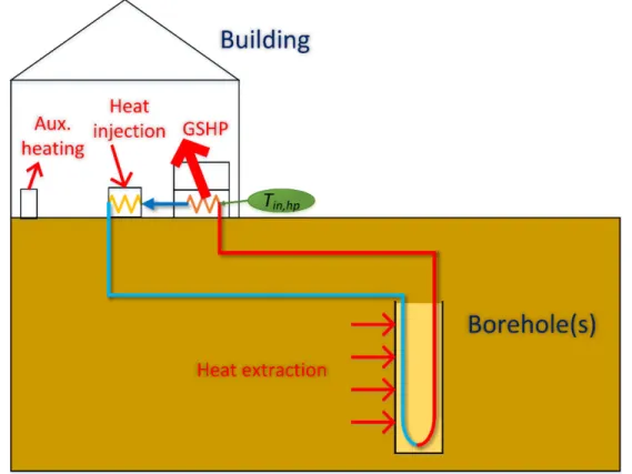
The self-assisted GSHP system considered in this paper is shown in Figure 1. The GSHP is coupled to a bore field and provides heating and cooling to a single-family dwelling. Figure 1 shows the operation
during the heating season. The GSHP is coupled to a bore field consisting of a single borehole. The heat pump is equipped with an electric element at its source-side outlet to provide assistance when approaching peak power demand. An auxiliary heater provides additional heating to the building when the heat pump cannot operate. The thermal assistance is meant to avoid the use of this auxiliary heating by keeping the returning fluid temperature (𝑇𝑖𝑛,ℎ𝑝) above a minimum temperature limit.
Figure 1. Self-assisted GSHP system
The operation of the heat injection element in the self-assisted GSHP depends on a model predictive control strategy. At regular intervals of 12 hours (i.e. the control period), the controller optimizes the operation of the heat injection element, providing the heat injection pattern at every controller time step (e.g. 15 minutes) of the 6 following days (i.e. the prediction horizon). In this paper, the control period corresponds to the frequency of update of the weather forecasts and the length of the prediction horizon corresponds to the length of the available weather forecasts. In a previous study (Laferrière and Cimmino, 2018), it was shown that heat injection should start several days ahead to eliminate auxiliary heating with minimal energy use. For the sake of controller simplicity, feasability and computation times, it is preferable for the model used in the predictive controller to rely on linear dynamics. However, the real-life operation
of a GSHP features many non-linearities. Thus, there is a distinction between the system emulation model, which simulates the system shown in Figure 1 as realistically as possible, and the control model, which is used by the controller as a linear approximation of the system for the sake of heat injection optimization. The components of the emulation model are presented in the next section, followed by the components of the control model.
Emulation model
The components of the emulation model are all developed in the Modelica language. Modelica is a modular object-oriented programming language aimed at simulating dynamic engineering systems (thermal, mechanical, electrical, etc.).
Building
The building is a single-family two-story residential dwelling in Montreal, Canada, with a total floor area of 200 m2. The Modelica building model was generated using the TEASER tool (Remmen et al., 2017). The TEASER tool generates building archetypes based on the energy performance of buildings in Germany. It was still used for the emulator because, to the authors’ knowledge, it is currently the only Modelica building archetype for single-family residential dwellings. To compensate for the differences in the typical energy performances of German and Canadian houses, the equivalent thermal resistances of the envelope elements (exterior walls, roof, floor plate and windows) were adjusted to the arithmetic mean of the base archetype value and the value prescribed by a local high-performance building code (Transition Énergétique Québec, 2018). The annual heating energy demand of the building model simulated with a typical meteorological year in Montreal is 72.4 kWh/m2/year. For a recently built house with very good energy performance, this value seems coherent, as Natural Resources Canada (2004) gives a value of about 119.5 kWh/m2/year for an average Montreal house built after 1990 (assuming a total floor area of 186 m2).
Bore field
The emulation model uses the bore field model developped by Laferrière et al. (submitted manuscript, 2018) and implemented into the open-source IBPSA library of building system models (“IBPSA Project 1,” n.d.). This model is comprised of two heat transfer regions: the long-term heat transfer in the ground surrounding the boreholes, and the short-term heat transfer through the borehole filling material and the
heat carrier fluid. The borehole wall temperature, considered uniform along the length of the boreholes, acts as an interface between the two regions. Temporal superposition of the bore field’s thermal response factor is used to evaluate the borehole wall temperature variation, with a load aggregation method to reduce calculation times. This method allows the model to simulate any number of boreholes positioned in any configuration. The thermal response factor, or g-function (Eskilson, 1987), is evaluated using a finite line source solution (Cimmino and Bernier, 2014; Cimmino, 2018) and is then corrected to account for the cylindrical geometry of boreholes (Li et al., 2014). The heat transfer through the grout, pipes and fluid uses a vertical discretization of a single equivalent borehole (as all of the boreholes are considered to have the same average borehole wall temperature). Each vertical element is modeled as a resistance-capacitance network (Bauer et al., 2011). The multipole method is used to calculate borehole resistances (Claesson and Hellström, 2011). In the radial direction, each element accounts for the fluid convective heat transfer (including the fluid thermal capacitance), the pipe conductive heat transfer, and the grout conductive heat transfer (including the grout thermal capacitance). In the axial direction, the heat transfer is strictly advective (i.e. due to the fluid flow). The bore field model was validated for both its short-term and long-term behaviour using a combination of analytical, experimental and field results.
GSHP
The heat pump is single-speed and reversible. Its energy performance is modeled based on the curve fitting equations proposed by Tang (2005) for water-to-air heat pumps. These equations use the source-side water inlet temperature 𝑇𝑖𝑛,ℎ𝑝, the source-side volumetric flow rate 𝑉̇𝑖𝑛,ℎ𝑝, the load-side dry-bulb (𝑇𝑏𝑢𝑖) and
wet-bulb (𝑇𝑤𝑏) temperatures, and the load-side volumetric flow rate 𝑉̇𝑏𝑢𝑖. The outputs are the capacity 𝑄
and the compressor input power 𝑃.
𝑄𝑐 𝑄𝑐,𝑟𝑒𝑓= B1 + B2 𝑇𝑏𝑢𝑖 𝑇𝑟𝑒𝑓+ B3 𝑇𝑤𝑏 𝑇𝑟𝑒𝑓+ B4 𝑇𝑖𝑛,ℎ𝑝 𝑇𝑟𝑒𝑓 + B5 𝑉̇𝑏𝑢𝑖 𝑉̇𝑏𝑢𝑖,𝑟𝑒𝑓,𝑐+ B6 𝑉̇𝑖𝑛,ℎ𝑝 𝑉̇𝑖𝑛,ℎ𝑝,𝑟𝑒𝑓,𝑐 (1) 𝑃𝑐 𝑃𝑐,𝑟𝑒𝑓= C1 + C2 𝑇𝑤𝑏 𝑇𝑟𝑒𝑓+ C3 𝑇𝑖𝑛,ℎ𝑝 𝑇𝑟𝑒𝑓 + C4 𝑉̇𝑏𝑢𝑖 𝑉̇𝑏𝑢𝑖,𝑟𝑒𝑓,𝑐+ C5 𝑉̇𝑖𝑛,ℎ𝑝 𝑉̇𝑖𝑛,ℎ𝑝,𝑟𝑒𝑓,𝑐 (2) 𝑄ℎ 𝑄ℎ,𝑟𝑒𝑓= E1 + E2 𝑇𝑏𝑢𝑖 𝑇𝑟𝑒𝑓+ E3 𝑇𝑖𝑛,ℎ𝑝 𝑇𝑟𝑒𝑓 + E4 𝑉̇𝑏𝑢𝑖 𝑉̇𝑎𝑖𝑟,𝑟𝑒𝑓,ℎ+ E5 𝑉̇𝑖𝑛,ℎ𝑝 𝑉̇𝑤,𝑟𝑒𝑓,ℎ (3) 𝑃ℎ 𝑃ℎ,𝑟𝑒𝑓= F1 + F2 𝑇𝑏𝑢𝑖 𝑇𝑟𝑒𝑓+ F3 𝑇𝑖𝑛,ℎ𝑝 𝑇𝑟𝑒𝑓 + F4 𝑉˙𝑏𝑢𝑖 𝑉̇𝑏𝑢𝑖,𝑟𝑒𝑓,ℎ+ F5 𝑉˙𝑖𝑛,ℎ𝑝 𝑉̇𝑖𝑛,ℎ𝑝,𝑟𝑒𝑓,ℎ (4)
The subscripts 𝑐 and ℎ refer to cooling and heating modes, respectively. Coefficients B1 to B6, C1 to C5, E1 to E5 and F1 to F5 are obtained via a curve fitting procedure using manufacturer data for a
residential GSHP with a nominal capacity of 11.13 kW. The manufacturer data also provides the reference conditions for Equations 1 to 4, i.e. the maximum capacities and their associated power consumptions and volumetric flow rates, while 𝑇𝑟𝑒𝑓 is set to 283 K as recommended by Tang (2005).
The capacity and the compressor power are used to calculate the the heat’s pump coefficient of performance (COP) for either heating (ℎ) or cooling (𝑐) modes.
COPℎ/𝑐= 𝑄ℎ/𝑐
𝑃ℎ/𝑐 (5)
The heat extraction or injection rate from the bore field can then be defined using this COP. 𝑄𝑠𝑜𝑢,ℎ= −𝑄ℎ(1 − 1 COPℎ) (6) 𝑄𝑠𝑜𝑢,𝑐= 𝑄𝑐(1 + 1 COP𝑐) (7)
where the heating and cooling capacities are positive and where 𝑄𝑠𝑜𝑢 is positive for heat injection into the
bore field (and negative for extraction).
The heat pump uses a hysteresis controller to maintain the indoor temperature above a heating setpoint of 21 °C and under a cooling setpoint of 24 °C. Both setpoints have a deadband of 2 °C around the setpoint. In all cases, to avoid excess compressor cycling, the heat pump must remain on for at least 3 minutes before being turned off again, and must remain off for at least 4 minutes before being turned on again. These values are provided in the manufacturer data.
The source-side heat carrier fluid is a 20% propylene-glycol mixture. The minimum source-side inlet temperature in heating mode is set to 0 °C to avoid the fluid potentially freezing at the heat pump source-side outlet. The maximum source-source-side inlet temperature in cooling mode is set to 50 °C, though this limit is never reached in the case being studied.
Other heating sources
As the heat pump uses the “self-assisted” heat pump configuration, heat injection into the ground is supplemented by a heating element located at the heat pump source-side outlet. The heating element, assumed to have negligible thermal losses, is controlled using model predictive control to recharge the ground in preparation of high heat demand periods and to avoid using the auxiliary heater. Should the heat injection fail to prevent the GSHP from shutting off due to a low source-side inlet temperature, the building will gradually cool down until it reaches the auxiliary heating setpoint of 19.5 °C. When this temperature is
reached, a hysteresis controller is used with a deadband of 1 °C to maintain the indoor temperature above the setpoint until the heat pump can safely operate.
Control model
Weather forecasts
One of the objectives of this paper is to include real weather forecasts in the control strategy and therefore account for the mismatch between weather forecasts and actual weather. Weather forecasts at the international airport in Montreal were collected over a period of a year, from October 26th, 2017 to November 1st, 2018. The weather forecasts are retrieved from two sources: CanMETEO (Candanedo et al., 2018) and Environment Canada (“Environment Canada,” n.d.). The CanMETEO software provides hourly ambient temperature forecasts, but is limited to a maximum horizon of 48 hours. In practice, as the forecasts are only updated every few hours, the forecasts are often less than 48 hours long. Hourly forecasts are linearly interpolated to sub-hourly intervals when required. To increase the precision of the forecasts while also having a sufficiently long prediction horizon, the CanMETEO forecasts were used for short-term predictions, and the Environment Canada forecasts for long-term predictions. However, forecasts provided by Environment Canada are limited to daily high and low temperatures and must first be converted to a time-varying temperature profile.
Synthetic hourly ambient temperature profiles are generated according to the method presented by De Wit (1978) and validated by Reicosky et al. (1989). This method assumes that the daily maximum ambient temperature occurs at 14:00 while the daily minimum temperature occurs at sunrise. At any given ℎ𝑜𝑢𝑟 of the day, the forecasted temperature 𝑇𝑎𝑚𝑏(ℎ𝑜𝑢𝑟) can be predicted using the nearest daily minimum
temperature 𝑇𝑎𝑚𝑏,𝑚𝑖𝑛, the nearest daily maximum temperature 𝑇𝑎𝑚𝑏,𝑚𝑎𝑥, and the sunrise time 𝑟𝑖𝑠𝑒.
𝑇𝑎𝑣𝑒= 𝑇𝑎𝑚𝑏,𝑚𝑎𝑥+𝑇𝑎𝑚𝑏,𝑚𝑖𝑛 2 (8) 𝑇𝑎𝑚𝑝= 𝑇𝑎𝑚𝑏,𝑚𝑎𝑥−𝑇𝑎𝑚𝑏,𝑚𝑖𝑛 2 (9) 𝑇𝑎𝑚𝑏(ℎ𝑜𝑢𝑟) = { 𝑇𝑎𝑣𝑒+ 𝑇𝑎𝑚𝑝cos(𝜋 ℎ𝑜𝑢𝑟+10 𝑟𝑖𝑠𝑒+10) ℎ𝑜𝑢𝑟 < 𝑟𝑖𝑠𝑒 𝑇𝑎𝑣𝑒− 𝑇𝑎𝑚𝑝cos(𝜋 ℎ𝑜𝑢𝑟−𝑟𝑖𝑠𝑒 14−𝑟𝑖𝑠𝑒 ) 𝑟𝑖𝑠𝑒 ≤ ℎ𝑜𝑢𝑟 ≤ 14 𝑇𝑎𝑣𝑒+ 𝑇𝑎𝑚𝑝cos(𝜋 ℎ𝑜𝑢𝑟−14 𝑟𝑖𝑠𝑒+10) 14 < ℎ𝑜𝑢𝑟 (10)
The Environment Canada forecasts were collected twice daily on a personal computer at intervals of 12 hours: once in the morning, once in the afternoon. The CanMETEO forecasts were collected once daily in the afternoon. Occasional technical problems such as electrical blackouts caused some forecasts to be missing. The missing Environment Canada forecasts were filled in by linearly interpolating between the two nearest forecasts for the same target time. Suppose, for example, that the forecasts could not be collected on January 1st at 14:00. Using the 2-day-ahead forecast (i.e. the forecast for January 3rd at 14:00) as an example, the missing forecast could be linearly interpolated with the forecasts for January 3rd at 14:00 that were collected on January 1st in the morning and on January 2nd in the morning. As for missing CanMETEO forecasts, these were instead replaced by the Environment Canada forecasts.
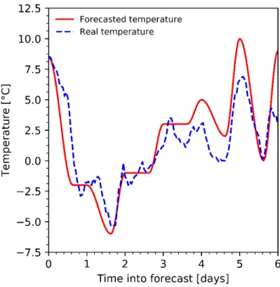
The starting points of every control period were set to 2:00 and 14:00. The boundary between the short-term and long-term forecasts was set at the first sunrise after the second full day. The time period of the forecasts varies between 6 and 7 days. To ensure a constant prediction horizon, the prediction horizon was fixed at 6 days, as this way all control periods could have the exact same prediction horizon. Figure 2 shows the contribution of both data sources to the generation of a 6-day-long hour-by-hour forecast using the forecasts of November 1st 2017 as an example. Each full day into the forecast ends at 14:00, and each dashed vertical bar represents a sunrise (at a different time each day). In the first region, wherein the forecasts are provided by CanMETEO, the maxima and minima do not necessarily align with day starts or sunrises. In the second region, wherein the forecasts are provided by Environment Canada, the day starts and sunrises are aligned with maxima and minima, respectively. Figures 3 and 4 show sample ambient temperature forecasts over the 6-day prediction horizon compared to the corresponding reported measured temperature. Figure 3, showing the forecast on the 7th of May 2018, is representative of clear sky periods with a root mean square difference of 2.13 ºC between the predicted and reported temperatures. Figure 4, showing the forecast on the 13th of April 2018, is representative of cloudy periods with some missing (i.e. interpolated) forecasts with a root mean square difference of 2.05 ºC between the predicted and reported temperatures.
Figure 2. Construction of 6-day-ahead weather forecasts on 2017-11-01
Figure 4. Comparison of forecasted and real temperatures, 2018-04-13
Building load forecasts
For a linear MPC formulation, the heat pump operation needs to be expressed as a linear function of the forecasted ambient temperature. This is a challenging task in the case of an on-off single-speed heat pump, as a regular time discretization of the order of minutes cannot accurately predict a heat pump’s cycling with highly variable operation times. Additionally, it also requires forecasts on solar gains (which were not collected during the year of forecast collection) and occupancy gains. Thus, the heat pump’s
average operating load is instead predicted using weather forecasts. The discretized average load is
expressed in two linear parts as a function of the difference between the indoor building temperature 𝑇𝑏𝑢𝑖
(assumed to be equal to the heating setpoint of 21 °C) and the ambient temperature 𝑇𝑎𝑚𝑏. This approach
provides an approximation of the solar gains and the occupancy gains directly within the building effective UA value. 𝑄𝑙𝑜𝑎𝑑(𝑘) = { 𝑈𝐴(𝑇𝑏𝑢𝑖− 𝑇𝑎𝑚𝑏(𝑘)) + 𝑞 𝑇𝑎𝑚𝑏≤ 𝑇𝑒𝑞,1 𝑈𝐴(𝑇𝑏𝑢𝑖−𝑇𝑒𝑞,1)+𝑞 (𝑇𝑒𝑞,2−𝑇𝑒𝑞,1) (𝑇𝑒𝑞,2− 𝑇𝑎𝑚𝑏(𝑘)) 𝑇𝑒𝑞,1< 𝑇𝑎𝑚𝑏≤ 𝑇𝑒𝑞,2 0 𝑇𝑒𝑞,2< 𝑇𝑎𝑚𝑏 (11)
The effective UA value, its associated load constant 𝑞, and the equilibrium temperatures (𝑇𝑒𝑞,1 and 𝑇𝑒𝑞,2)
were identified for two time periods: one set for daytime operation (7:00 to 19:00) and one set for nighttime operation (19:00 to 7:00), meaning that a total of 2 different UA values were used (𝑈𝐴𝑑𝑎𝑦 and 𝑈𝐴𝑛𝑖𝑔ℎ𝑡).
This was done by simulating the emulator model for a full year with a typical meteorological year and then using a curve fitting procedure with the half-day-averaged ambient temperatures and heating loads. The data points as well as the resulting curves are shown in Figure 5. The daytime half-day averaged heatings loads are shown as a function of the average ambient temperature in Figure 5a, while Figure 5b shows the nighttime half-day averaged loads. For ambient temperatures lower than 𝑇𝑒𝑞,1, which correspond to
temperatures at which auxiliary heating and heat injection are probable, the root-mean-square errors for Figures 5a and 5b are 773 W and 373 W, respectively. 𝑇𝑒𝑞,1 is equal to -2.85 °C for the daytime curve fit
and 1.35 °C for the nighttime curve fit. The lack of solar gains and the more regular occupancy gains at night explain why the nighttime curve fit displays a better fit.
Figure 5. Building heating load curve fitting
To model the bore field thermal dynamics, a hybrid numerical/semi-analytical approach is proposed. The approach uses a bore field’s “ground-to-fluid thermal response factor” (GTFTRF). The GTFTRF is similar to more conventional thermal response factors (e.g. g-functions), with the difference that the thermal response extends to the average fluid temperature rather than the borehole wall temperature. In other words, it includes short-term thermal capacity effects. The GTFTRF gives the variation of the mean fluid temperature in the bore field in response to a constant total heat injection rate into the bore field. It is defined by the relation:
𝑇𝑓(𝑡) = 𝑇𝑔+ 𝑔𝑔𝑓(𝑡)
2𝜋ℎ𝑘𝑠𝑁𝑏∙ 𝑄 (12)
where 𝑇𝑓 = 1
2(𝑇𝑖𝑛,𝑠𝑜𝑢+ 𝑇𝑜𝑢𝑡,𝑠𝑜𝑢) is the arithmetic mean fluid temperature in the bore field, 𝑇𝑖𝑛,𝑠𝑜𝑢 and
𝑇𝑜𝑢𝑡,𝑠𝑜𝑢 are the inlet and outlet fluid temperature in the bore field, 𝑇𝑔 is the undisturbed ground temperature,
𝑄 is a constant total heat injection rate, 𝑔𝑔𝑓 is the GTFTRF, ℎ is the borehole length, 𝑘𝑠 is the ground
thermal conductivity, and 𝑁𝑏 is the number of boreholes in the bore field.
The mean fluid temperature variation due to a varying heat injection rate into the bore field is obtained from the temporal superposition of the GTFTRF. At a time 𝑘:
𝑇𝑓(𝑘) = 𝑇𝑔(𝑘) + 1
2𝜋ℎ𝑘𝑠𝑁𝑏∑ (𝑔𝑔𝑓(𝑘 − 𝑖 + 1) − 𝑔𝑔𝑓(𝑘 − 𝑖)) 𝑄(𝑖)
𝑘
𝑖=1 (13)
The summation in Equation 13 becomes computationally intensive in multi-year simulations with small time steps. Therefore, a modified cell-shifting aggregation scheme based on the work of Claesson and Javed (2012) is used instead. The cell-shifting load aggregation scheme involves discretizing the thermal history of the bore field since the start of the system’s operation into 𝑁𝑐 cells. Each cell 𝑖 represents the
average ground thermal load during a period spanning from 𝜈𝑖−1 to 𝜈𝑖 of the bore field’s thermal history.
The 𝑤𝑖𝑑𝑡ℎ𝑖 of each cell doubles every 𝑛𝑐 cells, meaning more distant cells contain thermal loads averaged
over longer time periods. The widths and time spans of each cell are defined by: 𝑤𝑖𝑑𝑡ℎ𝑖= 2floor( 𝑖−1 𝑛𝑐) (14) 𝜈𝑖= Δ𝑡 ∑ 𝑤𝑖𝑑𝑡ℎ𝑗 𝑖 𝑗=1 (15)
i.e. 𝜈𝑖= 𝜈𝑖−1+ Δ𝑡 ∙ 𝑤𝑖𝑑𝑡ℎ𝑖 with 𝜈0= 0, where Δ𝑡 is the controller time step. At every controller time step,
controller time step 𝑘 occuring at time 𝑡, the value of the aggregated load 𝑄̅𝑖
(𝑘) of each cell 𝑖 ≥ 2 is
expressed as a function of aggregated loads from controller step (𝑘 − 1):
𝑄̅𝑖≥2(𝑘) = { 0 𝑡 < 𝜈𝑖−1 1 𝑤𝑖𝑑𝑡ℎ𝑖𝑄̅𝑖−1 (𝑘−1) + 𝑄̅𝑖(𝑘−1) 𝜈𝑖−1≤ 𝑡 < 𝜈𝑖 1 𝑤𝑖𝑑𝑡ℎ𝑖𝑄̅𝑖−1 (𝑘−1) +𝑤𝑖𝑑𝑡ℎ𝑖−1 𝑤𝑖𝑑𝑡ℎ𝑖 𝑄̅𝑖 (𝑘−1) 𝜈𝑖≤ 𝑡 (16)
The value of the averaged ground load in the first cell, 𝑄̅1 (𝑘)
, is equal to the ground load during the current controller time step, 𝑄(𝑘).
The aggregation weighting factor 𝜅 of each cell 𝑖 is then calculated using the GTFTRF: 𝜅𝑖=
1
2𝜋ℎ𝑘𝑠𝑁𝑏(𝑔𝑔𝑓(𝜈𝑖) − 𝑔𝑔𝑓(𝜈𝑖−1)) (17)
with 𝑔𝑔𝑓(𝜈0) = 0. At each controller time step 𝑘, temporal superposition is performed on the averaged
ground loads to determine the mean fluid temperature: 𝑇𝑓(𝑘) = 𝑇𝑔(𝑘) + ∑ 𝜅𝑖𝑄𝑖
(𝑘) 𝑁𝑐
𝑖=1 (18)
GSHP performance prediction
Contrary to the emulation model, the GSHP’s energy performance in the control model should strictly rely on variables which can be measured or predicted. Thus, the control model assumes that the load-side temperature, the load-side volumetric flow rate and the source-side volumetric flow rate are all constant and known, leaving the source-side heat pump inlet temperature 𝑇𝑖𝑛,ℎ𝑝 (= 𝑇𝑜𝑢𝑡,𝑠𝑜𝑢) as the only variable
taken into account. Manufacturer data was used to produce a quadratic curve fit.
𝐶𝑂𝑃(𝑘) = 𝛽1+ 𝛽2𝑇𝑖𝑛,ℎ𝑝(𝑘) + 𝛽3𝑇𝑖𝑛,ℎ𝑝2 (𝑘) (19)
where 𝛽1, 𝛽2 and 𝛽3 are the curve fit coefficients. Assuming steady state heat pump behaviour, 𝑇𝑖𝑛,ℎ𝑝 is
calculated using 𝑇𝑓 and the ground load 𝑄.
𝑇𝑖𝑛,ℎ𝑝(𝑘) = 𝑇𝑓(𝑘) − 𝑄(𝑘) 2𝑚̇𝑐𝑝 (20a) 𝑇𝑖𝑛,ℎ𝑝(𝑘)= 𝑇𝑓(𝑘) − (𝑄𝑖𝑛𝑗(𝑘)−𝑄𝑠𝑜𝑢(𝑘)) 2𝑚̇𝑐𝑝 (20b) 𝑇𝑖𝑛,ℎ𝑝(𝑘)= 𝑇𝑓(𝑘) − (𝑄𝑖𝑛𝑗(𝑘)−(1−𝐶𝑂𝑃(𝑘)1 )𝑄𝑙𝑜𝑎𝑑(𝑘)) 2𝑚̇𝑐𝑝 (20c)
where 𝑄𝑖𝑛𝑗 is the heat injection in the self-assisted configuration, 𝑚̇ is the source-side mass flow rate, and
𝑐𝑝 is the specific heat capacity of the heat carrier fluid.
MPC formulation
MPC relies on a model to forecast future system dynamics based on future input signals and forecasted disturbances. In this section, a brief theoretical framework for linear time-varying (LTV) MPC with a state space representation is first provided, followed by a LTV state space representation of the self-assited GSHP system.
LTV MPC framework
With a discrete linear state space representation, the vector of states 𝑥 changes from time step 𝑘 to 𝑘 + 1 following 𝑢𝑘, a vector of input signals, and 𝑤𝑘, a vector of input disturbances.
𝑥𝑘+1= 𝐴𝑘𝑥𝑘+ 𝐵𝑘𝑢𝑘+ 𝐸𝑘𝑤𝑘 (21)
where the matrices 𝐴𝑘, 𝐵𝑘 and 𝐸𝑘 provide the system dynamics at time 𝑘. Provided forecasts on the future
values of the 𝑢 and 𝑤 vectors as well as knowledge of the future 𝐴, 𝐵 and 𝐸 matrices, the future states 𝑥 predicted at time 𝑘 can be expressed through successive applications of Equation 21:
𝑋𝑘 = Γ𝑘𝑥𝑘+ 𝐻𝑘𝑢𝑈𝑘+ 𝐻𝑘𝑤𝑊𝑘 (22) 𝑋𝑘 = [ 𝑥𝑘+1|𝑘 𝑥𝑘+2|𝑘 𝑥𝑘+3|𝑘 ⋮ 𝑥𝑘+𝑁𝑝|𝑘] (23) Γ𝑘= [ 𝐴𝑘 𝐴𝑘+1𝐴𝑘 𝐴𝑘+2𝐴𝑘+1𝐴𝑘 ⋮ ∏0𝑖=𝑁𝑝−1𝐴𝑘+𝑖] (24) 𝐻𝑘𝑢= [ 𝐵𝑘 0 0 … 𝐴𝑘+1𝐵𝑘 𝐵𝑘+1 0 … 𝐴𝑘+2𝐴𝑘+1𝐵𝑘 𝐴𝑘+2𝐵𝑘+1 𝐵𝑘+2 … ⋮ ⋮ ⋮ ⋮ (∏1𝑖=𝑁𝑝−1𝐴𝑘+𝑖)𝐵𝑘 (∏ 𝐴𝑘+𝑖 2 𝑖=𝑁𝑝−1 )𝐵𝑘+1 (∏ 𝐴𝑘+𝑖 3 𝑖=𝑁𝑝−1 )𝐵𝑘+2 …] (25) 𝑈𝑘= [ 𝑢𝑘|𝑘 𝑢𝑘+1|𝑘 𝑢𝑘+2|𝑘 ⋮ 𝑢𝑘+𝑁𝑝−1|𝑘] (26)
𝐻𝑘𝑤= [ 𝐸𝑘 0 0 … 𝐴𝑘+1𝐸𝑘 𝐸𝑘+1 0 … 𝐴𝑘+2𝐴𝑘+1𝐸𝑘 𝐴𝑘+2𝐸𝑘+1 𝐸𝑘+2 … ⋮ ⋮ ⋮ ⋮ (∏1𝑖=𝑁𝑝−1𝐴𝑘+𝑖)𝐸𝑘 (∏ 𝐴𝑘+𝑖 2 𝑖=𝑁𝑝−1 )𝐸𝑘+1 (∏ 𝐴𝑘+𝑖 3 𝑖=𝑁𝑝−1 )𝐸𝑘+2 …] (27) 𝑊𝑘= [ 𝑤𝑘|𝑘 𝑤𝑘+1|𝑘 𝑤𝑘+2|𝑘 ⋮ 𝑤𝑘+𝑁𝑝−1|𝑘] (28)
where 𝑁𝑝 is the number of controller time steps in the prediction horizon and 𝑋𝑘, 𝑈𝑘 and 𝑊𝑘 are vectors of
vectors wherein the |𝑘 subscript denotes vectors that are predicted (𝑥, 𝑤) or optimized (𝑢) at time 𝑘. The presence of the term 𝑥𝑘 in Equation 22 indicates that the initial conditions of the states are appropriately
reset at the start of every control period.
LTV MPC applied to a GSHP
This section presents a LTV state space formulation to predict the inlet fluid temperature and to use the heat injection element of the self-assisted configuration to prevent the use of auxiliary heating. This first requires the prediction of the mean bore field fluid temperature with the general format shown in Equation 21. The bore field’s aggregated ground loads 𝑄̅ are used as the state variables with the dynamics shown in Equation 18 as well as the decomposition of the total ground load shown in Equation 20.
𝑥𝑘 = [ 𝑄1 (𝑘) 𝑄2(𝑘) 𝑄3(𝑘) ⋮ 𝑄𝑁(𝑘)𝑐] (29) 𝑢𝑘= [𝑄𝑖𝑛𝑗(𝑘)] (30) 𝑤𝑘= [𝑄𝑙𝑜𝑎𝑑(𝑘)] (31)
The matrices defining the discrete system dynamics are derived from the dynamics shown in the control model section.
𝐴𝑘= [ 0 0 0 0 ⋯ 𝑎2,1(𝑘) 𝑎2,2(𝑘) 0 0 ⋯ 0 𝑎3,2(𝑘) 𝑎3,3(𝑘) 0 ⋯ 0 0 𝑎4,3(𝑘) 𝑎4,4(𝑘) ⋯ ⋮ ⋮ ⋮ ⋮ ⋮ ]𝑁𝑐×𝑁𝑐 (32)
𝑎𝑖,𝑖−1(𝑘) = { 0 𝑘Δ𝑡 < 𝜈𝑖−1 1 𝑤𝑖𝑑𝑡ℎ𝑖 𝑘Δ𝑡 ≥ 𝜈𝑖−1 (33) 𝑎𝑖,𝑖(𝑘) = { 0 𝑘Δ𝑡 < 𝜈𝑖−1 1 𝜈𝑖−1≤ 𝑘Δ𝑡 < 𝜈𝑖 𝑤𝑖𝑑𝑡ℎ𝑖−1 𝑤𝑖𝑑𝑡ℎ𝑖 𝜈𝑖≤ 𝑘Δ𝑡 (34) 𝐵𝑘 = [ 1 0 0 ⋮ 0]𝑁𝑐×1 (35) 𝐸𝑘= [ −(1 − 1 𝐶𝑂𝑃(𝑘)) 0 0 ⋮ 0 ]𝑁𝑐×1 (36)
The 𝑁𝑝-step-ahead aggregated ground loads can then be predicted with the formulation used in
Equation 22, after which they can be used to predict the 𝑁𝑝-step-ahead fluid temperatures following the
temporal superposition shown in Equation 18. 𝑇→𝑓(𝑘) = 𝑉 [Γ⏟ 𝑘𝑥𝑘+ 𝐻𝑘𝑢𝑈𝑘+ 𝐻𝑘𝑤𝑊𝑘] 𝑋𝑘 + 𝑇→𝑔 (37) 𝑇→𝑓(𝑘) = [ 𝑇𝑓(𝑘 + 1) 𝑇𝑓(𝑘 + 2) 𝑇𝑓(𝑘 + 3) ⋮ 𝑇𝑓(𝑘 + 𝑁𝑝)] (38) 𝑇 → 𝑔(𝑘) = [ 𝑇𝑔(𝑘 + 1) 𝑇𝑔(𝑘 + 2) 𝑇𝑔(𝑘 + 3) ⋮ 𝑇𝑔(𝑘 + 𝑁𝑝)] (39) 𝑉 = [ 𝜔 0 0 ⋯ 0 0 𝜔 0 ⋯ 0 0 0 𝜔 ⋯ 0 ⋮ ⋮ ⋮ ⋮ ⋮ 0 0 0 ⋯ 𝜔] (40) 𝜔 = [𝜅1 𝜅2 𝜅3 ⋯ 𝜅𝑁𝑐] (41)
where 𝑇→𝑓 is the vector of all mean fluid temperatures 𝑇𝑓 in the prediction horizon. Similarly, 𝑇 →
𝑔 is the vector
of all undisturbed ground temperatures 𝑇𝑔 in the prediction horizon. In this paper, 𝑇𝑔 is assumed to be
constant.
Control-oriented COP dynamics
The presence of the 𝐶𝑂𝑃(𝑘) term in Equation 36 renders the formulation non-linear, as the COP depends on the state variables in a non-linear fashion. Therefore, an iterative approach is proposed whereby the COP at each controller time step is evaluated iteratively. The COP is evaluated from the inlet fluid temperature to the heat pump at each iteration based on the latest prediction of mean fluid temperatures. This process is repeated until convergence, i.e. until the maximum difference between the assumed COP values and the calculated COP values falls below the absolute COP tolerance 𝜀𝐶𝑂𝑃. The inlet fluid
temperatures to the heat pump in the prediction horizon are given by: 𝑇→𝑖𝑛,ℎ𝑝(𝑘) = 𝑇 → 𝑓(𝑘) + 𝐻Δ𝑇,𝑢𝑈𝑘+ 𝐻Δ𝑇,𝑤𝑊𝑘 (42) 𝑇→𝑖𝑛,ℎ𝑝(𝑘) = [ 𝑇𝑖𝑛,ℎ𝑝(𝑘 + 1) 𝑇𝑖𝑛,ℎ𝑝(𝑘 + 2) 𝑇𝑖𝑛,ℎ𝑝(𝑘 + 3) ⋮ 𝑇𝑖𝑛,ℎ𝑝(𝑘 + 𝑁𝑝)] (43) 𝐻Δ𝑇,𝑢= [ −1 2𝑚̇𝑐𝑝 0 0 ⋯ 0 −1 2𝑚̇𝑐𝑝 0 ⋯ 0 0 −1 2𝑚̇𝑐𝑝 ⋯ ⋮ ⋮ ⋮ ⋮ ] (44) 𝐻Δ𝑇,𝑤(𝑘) = [ (1−𝐶𝑂𝑃(𝑘)1 ) 2𝑚̇𝑐𝑝 0 0 ⋯ 0 (1− 1 𝐶𝑂𝑃(𝑘+1)) 2𝑚̇𝑐𝑝 0 ⋯ 0 0 (1− 1 𝐶𝑂𝑃(𝑘+2)) 2𝑚̇𝑐𝑝 ⋯ ⋮ ⋮ ⋮ ⋮ ] (45)
Optimization and cost function
The aim of the control strategy is to prevent 𝑇𝑓(𝑘) from falling below a certain minimum temperature
𝑇𝑚𝑖𝑛(𝑘). Here, 𝑇𝑓(𝑘), rather than 𝑇𝑖𝑛,ℎ𝑝(𝑘), is constrained to be maintained above the minimum
time step. As shown by Laferrière and Cimmino (2018), peak power consumption reduction can be achieved by eliminating auxiliary electric power, and thus by maintaining the mean fluid temperature above the low temperature limit. In this formulation, the sum of all 𝑄𝑖𝑛𝑗 values in the prediction horizon is
minimized while respecting state constraints and bounds on 𝑄𝑖𝑛𝑗 and 𝑇𝑓:
min 0≤𝑄𝑖𝑛𝑗(𝑘+𝑖|𝑘)≤𝑄𝑖𝑛𝑗,𝑚𝑎𝑥∑ 𝑄𝑖𝑛𝑗(𝑘 + 𝑖|𝑘) 𝑁𝑝−1 𝑖=0 s.t.[−𝑉𝐻𝑘𝑢]𝑈𝑘≤ [−𝑇 → 𝑚𝑖𝑛(𝑘) + 𝑉Γ𝑘𝑥𝑘+ 𝑉𝐻𝑘𝑤𝑊𝑘+ 𝑇 → 𝑔(𝑘)] (46)
where 𝑄𝑖𝑛𝑗,𝑚𝑎𝑥 is the upper bound on 𝑄𝑖𝑛𝑗. In this paper, the lower and upper bounds on 𝑄𝑖𝑛𝑗 are constant,
though they could also be time-varying. 𝑇→𝑚𝑖𝑛 is the vector of future minimum fluid temperatures entering
the heat pump.
𝑇→𝑚𝑖𝑛(𝑘) = [ 𝑇𝑚𝑖𝑛(𝑘 + 1) 𝑇𝑚𝑖𝑛(𝑘 + 2) 𝑇𝑚𝑖𝑛(𝑘 + 3) ⋮ 𝑇𝑚𝑖𝑛(𝑘 + 𝑁𝑝)] (47) Operational bounds
Due to the model’s reliance on imperfect weather forecasts and the averaged ground load prediction method shown in Equation 11, the control model is likely to exhibit some modelling error. In particular, the use of 𝑇𝑓 as a worst-case 𝑇𝑖𝑛,ℎ𝑝 detailed previously is likely to cause a systematic overestimation of the heat
injection requirements. While this helps to reduce auxiliary electric heating, it is also likely to cause an unnecessarily large increase in energy consumption. Therefore, 𝑇𝑚𝑖𝑛 is complemented by a Kalman filter to
minimize any systematic error of the GSHP source-side inlet temperature prediction and, therefore, minimize the amount of unnecessary heat injection into the bore field. The Kalman filter recursively attempts to correct the 𝑏𝑖𝑎𝑠 of 𝑇𝑖𝑛,ℎ𝑝. The 𝑏𝑖𝑎𝑠 is defined as the difference between the forecasted
temperature and the measured temperature, i.e. 𝑏𝑖𝑎𝑠 = 𝑓𝑜𝑟𝑒𝑐𝑎𝑠𝑡 − 𝑚𝑒𝑎𝑠𝑢𝑟𝑒. Here, only the maximum measured bias of 𝑇𝑖𝑛,ℎ𝑝 (i.e. the worst-case overestimation of 𝑇𝑖𝑛,ℎ𝑝) over the past control period is
considered and used as a measure of the bias for the Kalman filter. The filtered bias is denoted as 𝑏𝑖𝑎𝑠𝐾𝑎𝑙.
𝑇𝑚𝑖𝑛= 0℃ + 𝑏𝑖𝑎𝑠𝐾𝑎𝑙 (48)
The Kalman filter used in this paper follows the approach suggested by Galanis and Anadranistakis (2002), which involves a linear one-dimensional model to correct the bias in ambient air temperature
forecasts with a dynamic recalculation of the covariances of the process and output noises. The same initial conditions were used for the process noise covariance (i.e. 𝑄𝐾𝑎𝑙(0) = 1), the output noise covariance (i.e.
𝑅𝐾𝑎𝑙(0) = 6), the filter model state (i.e. 𝑧(0) = 0), and the filter model state’s error covariance (i.e.
𝑃(0) = 4). The number of samples 𝑁𝐾𝑎𝑙 before the noise covariances are recalculated is 6 (i.e. 3 days)
rather than 7 as used by Galanis and Anadranistakis (2002). As the Kalman filter is updated at the start of every control period, the value of 𝑏𝑖𝑎𝑠𝐾𝑎𝑙 is potentially different for every control period (though applied
uniformly to every control time step within a given prediction horizon).
The downside with this approach is that the Kalman filter is a reactive filter. This means that, when faced with any sudden changes in the systematic bias, it can only react one control period later at best. To anticipate situations where the application of the Kalman filter could lead to an under-injection of heat into the bore field, the measure of 𝑇𝑖𝑛,ℎ𝑝 at the start of a control period is used to verify whether or not the
GSHP is within a certain margin Δ𝑇𝑚𝑎𝑟𝑔𝑖𝑛 of the GSHP’s physical operational bounds.
Δ𝑇𝑚𝑎𝑟𝑔𝑖𝑛 = 𝑄𝑙𝑏
2𝑚̇𝑐𝑝 (49)
where 𝑄𝑙𝑏 is the ground load 𝑄 when 𝑇𝑖𝑛,ℎ𝑝 is near the GSHP’s lower limit. If the initial 𝑇𝑖𝑛,ℎ𝑝 is lower than
Δ𝑇𝑚𝑎𝑟𝑔𝑖𝑛, negative values of 𝑏𝑖𝑎𝑠𝐾𝑎𝑙 in Equation 48 are ignored. The definition of Δ𝑇𝑚𝑎𝑟𝑔𝑖𝑛 shown in
Equation 49 stems from the definition of the steady-state fluid temperature shown in Equation 20. Specifically, it is assumed that, should the operational bound of 0 °C be within a half-amplitude of the expected variation around the average 𝑇𝑓, the Kalman filter’s adjustment (𝑏𝑖𝑎𝑠𝐾𝑎𝑙) should be ignored for
any value 𝑏𝑖𝑎𝑠𝐾𝑎𝑙< 0.
Results
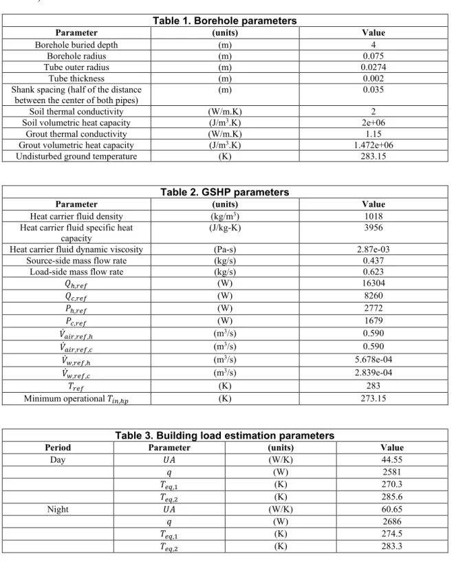
The methodology described in the previous section was used to study the performance of the described MPC strategy on a single-family two-story dwelling with a total floor area of 200 m2 in Montreal, Canada. The energy performance is studied over a simulation period of 20 years. As the weather forecasts were collected over a period of only one year, these forecasts were repeated from year to year. Along with the forecasts, the real weather data used by the emulation model covered the same period and was also repeated year to year. The building heating and cooling loads are primarily met by a GSHP with a bore field
consisting of one single-U-Tube vertical borehole. The borehole parameters are shown in Table 1, the emulation model GSHP parameters are shown in Table 2, the control model building load estimation parameters are shown in Table 3, and the GSHP curve fit coefficients (for the emulation and control models) are shown in Table 4.
Table 1. Borehole parameters
Parameter (units) Value
Borehole buried depth (m) 4
Borehole radius (m) 0.075
Tube outer radius (m) 0.0274
Tube thickness (m) 0.002
Shank spacing (half of the distance
between the center of both pipes) (m) 0.035
Soil thermal conductivity (W/m.K) 2
Soil volumetric heat capacity (J/m3.K) 2e+06
Grout thermal conductivity (W/m.K) 1.15
Grout volumetric heat capacity (J/m3.K) 1.472e+06
Undisturbed ground temperature (K) 283.15
Table 2. GSHP parameters
Parameter (units) Value
Heat carrier fluid density (kg/m3) 1018
Heat carrier fluid specific heat
capacity (J/kg-K) 3956
Heat carrier fluid dynamic viscosity (Pa-s) 2.87e-03
Source-side mass flow rate (kg/s) 0.437
Load-side mass flow rate (kg/s) 0.623
𝑄ℎ,𝑟𝑒𝑓 (W) 16304 𝑄𝑐,𝑟𝑒𝑓 (W) 8260 𝑃ℎ,𝑟𝑒𝑓 (W) 2772 𝑃𝑐,𝑟𝑒𝑓 (W) 1679 𝑉̇𝑎𝑖𝑟,𝑟𝑒𝑓,ℎ (m3/s) 0.590 𝑉̇𝑎𝑖𝑟,𝑟𝑒𝑓,𝑐 (m3/s) 0.590 𝑉̇𝑤,𝑟𝑒𝑓,ℎ (m3/s) 5.678e-04 𝑉̇𝑤,𝑟𝑒𝑓,𝑐 (m3/s) 2.839e-04 𝑇𝑟𝑒𝑓 (K) 283 Minimum operational 𝑇𝑖𝑛,ℎ𝑝 (K) 273.15
Table 3. Building load estimation parameters
Period Parameter (units) Value
Day 𝑈𝐴 (W/K) 44.55 𝑞 (W) 2581 𝑇𝑒𝑞,1 (K) 270.3 𝑇𝑒𝑞,2 (K) 285.6 Night 𝑈𝐴 (W/K) 60.65 𝑞 (W) 2686 𝑇𝑒𝑞,1 (K) 274.5 𝑇𝑒𝑞,2 (K) 283.3
Table 4. Heat pump curve fit coefficients 1 2 3 4 5 6 B 4.557 17.123 -20.265 -1.057 0.238 0.018 C -10.696 4.954 6.068 0.755 -0.141 - E -2.361 -0.865 3.815 0.027 0.113 - F -6.226 5.377 1.651 -0.220 0.057 - 𝛽 -98.600 0.659 -0.001 - - -
The emulation model uses variable simulation time steps. While the nominal time step is 300 seconds, this can become shorter whenever an event (e.g. a change in a controller’s input condition) is triggered. The control strategy uses a time step Δ𝑡 of 15 minutes, i.e. 900 seconds. The key parameters of the predictive controller are shown in Table 5, where 𝑁𝑐𝑡𝑟𝑙 refers to the number of control time steps within a control
period, i.e. the number of steps from a given total prediction horizon that are applied. Table 5. MPC parameters
Parameter (units) Value
Δ𝑡 (s) 900 𝑁𝐾𝑎𝑙 (-) 6 𝑁𝑐𝑡𝑟𝑙 (-) 48 𝑁𝑝 (-) 577 𝑄𝑖𝑛𝑗,𝑚𝑎𝑥 (W) 5000 Δ𝑇𝑚𝑎𝑟𝑔𝑖𝑛 (K) 1.9 𝑁𝑐 (-) 86
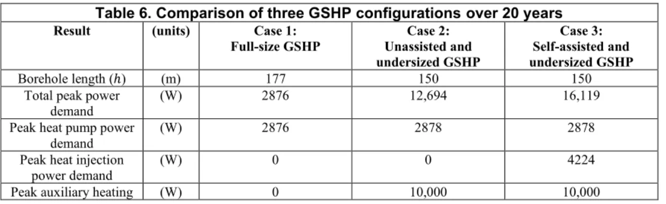
The energy performance of the proposed control strategy is studied by comparing three cases: (1) a GSHP system with a sufficiently long borehole to avoid any auxiliary heating over 20 years, (2) an undersized and unassisted GSHP with a shorter borehole and, therefore, auxiliary electric heating, and (3) a self-assisted undersized GSHP with the same shorter borehole. The auxiliary electric heating capacity is 10 kW in all three cases. The three cases are compared in Table 6. “Total peak power demand” and “total energy consumption” are calculated using the sum of the power demands or energy consumptions of the heat pump compressor, the assisting heat injection, and the auxiliary electric heating.
Table 6. Comparison of three GSHP configurations over 20 years
Result (units) Case 1:
Full-size GSHP Unassisted and Case 2: undersized GSHP
Case 3: Self-assisted and undersized GSHP
Borehole length (ℎ) (m) 177 150 150
Total peak power
demand (W) 2876 12,694 16,119
Peak heat pump power
demand (W) 2876 2878 2878
Peak heat injection
power demand (W) 0 0 4224
power demand Yearly average total
energy consumption (kWh) 4064 4329 4568
Yearly average heat pump energy consumption
(kWh) 4064 4049 4114
Yearly average heat injection energy consumption (kWh) 0 0 443 Yearly average auxiliary heating energy consumption (kWh) 0 279 11
The results in Table 6 show that the self-assisted GSHP (i.e. Case 3) does not fully eliminate auxiliary electric heating. Thus, when compared to a similar unassisted GSHP (i.e. Case 2), there is no decrease in peak power demand; rather, there is an increase in peak power demand as there are a few instances of combined auxiliary electric heating and heat injection. It is worth noting that the instances of such high demand are rare, as there is only a total of 1.1 hour per year of auxiliary electric heating during Case 3 (compared to 27.9 hours in Case 2). Therefore, while the overall peak power demand increases, the majority of peaks are decreased by at least 5 kW. Additionally, there is a net 239 kWh (i.e. 5.53%) increase in energy consumption. Indeed, while the average yearly auxiliary electric heating over 20 years decreases from 279 kWh to 11 kWh (i.e. -96%), the average required yearly heat injection is 443 kWh, which is greater than the decrease in auxiliary electric heating.
Figure 6 compares the total power demand of all three cases during the 20th year. Figure 6a shows the daily average total energy consumption, while Figure 6b shows the daily maximum power demand. While the highest peak power demand in Case 3 doesn’t decrease with regards to Case 2, there are fewer peaks of auxiliary electric heating. Therefore, rather than focusing on peak power demand over 20 years, the results instead focus on the amount of auxiliary electric heating over 20 years.
Figure 6. Total heating-related power demand, 20th year
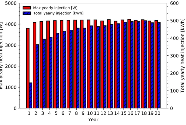
Figure 7 shows the yearly total and maximum heat injection for Case 3 that was found to be optimal by the model predictive controller, while Figure 8 shows the heat injection profile during the 20th year and compares the heat injection with the value of 𝑇𝑖𝑛,ℎ𝑝. The heat injection profile displays similar year-to-year
peaks after the first heating season. This can be explained by the fact that the system starts at a temperature equal to the undisturbed ground temperature, which is 10 °C in this paper. Thus, the GSHP requires less heat injection during the first year of operation. As for year-to-year total energy consumption, it reaches a steady value after approximately 16 years. Figure 8 shows that heat injection mainly coincides with low returning fluid temperatures.
Figure 8. Heat injection and returning fluid temperature, 20th year
A 4th Case is added to the comparison. This 4th Case is the same as Case 3, though without the 𝑏𝑖𝑎𝑠𝐾𝑎𝑙
adjustment from the Kalman filter. In other words, Case 4 has a constant 𝑇𝑚𝑖𝑛 of 0 °C. Table 7 compares
the energy performance of the undersized GSHPs, i.e. Cases 2, 3 and 4. Without the Kalman filter (i.e. in Case 4), the net increase in yearly average energy consumption is 322 kWh (7.45%), wich is greater than the increase of 239 kWh observed with the Kalman filter. This indicates that the absence of Kalman filter causes an overprediction of the heat injection required to eliminate the use of auxiliary electric heating. These results are as anticipated, as the Kalman filter attempts to correct the bias in fluid temperature predictions to generally reduce the amount of heat injection.
Table 7. Effect of the Kalman-filtered bias
Result (units) Case 2: Unassisted and undersized GSHP Case 3: Self-assisted and undersized GSHP Case 4: Self-assisted and undersized GSHP without 𝒃𝒊𝒂𝒔𝑲𝒂𝒍
Yearly average total
energy consumption (kWh) 4329 4568 4651 % change in total energy consumption relative to Case 2 (-) - +5.53% +7.45% Yearly average auxiliary electric heating consumption (kWh) 279 11 10 % change in auxiliary electric heating consumption relative to Case 2 (-) - -96% -96.2%
Yearly average heat
injection (kWh) 0 443 536
Calculation times
The total time required for the simulation of Case 3 to be completed on a PC was about 60.5 hours. However, the majority of this time (75%) was taken up by the emulation model due to the bore field model and the hysteresis controllers used for the heat pump operation. The total time taken by the MPC calculations (including the multiple COP iterations) over 20 years was about 15.2 hours. The average time for the MPC calculations for a single control period (once again including the multiple COP iterations) was 7.1 seconds, with a maximum value of 16.9 seconds. As the controller only optimizes a heat injection profile once every 12 hours, this is fast enough to be considered real-time. In Case 3, the COP convergence procedure described in the Methodology section succeeded in achieving convergence with a maximum of 4
iterations and an average of 3.98 iterations over 20 years. This was done with an absolute tolerance 𝜀𝐶𝑂𝑃 of
10-4.
Model parameter sensitivity
This section analyzes the sensitivity of the results to three parameters: heat pump heating load predictions (𝑄𝑙𝑜𝑎𝑑), the Kalman filter’s initial conditions (𝑃(0), 𝑄𝐾𝑎𝑙(0) and 𝑅𝐾𝑎𝑙(0)) and the frequency at
which the covariances in the Kalman filter are updated (𝑁𝐾𝑎𝑙). Table 8 compares the results of Case 3 with
the results from four new cases (5, 6, 7 and 8) with varied parameters. Table 8. Sensitivity analysis
Case Modified
parameter New value (% change) Yearly average total energy consumption (kWh) Yearly average heat injection energy consumption (kWh) Yearly average auxiliary electric heating energy consumption (kWh) Case 3 - - 4568 443 11 Case 5 𝑄𝑙𝑜𝑎𝑑 (+10%) 4667 554 3 Case 6 𝑄𝑙𝑜𝑎𝑑 (-10%) 4459 301 48 Case 7 𝑁𝐾𝑎𝑙 14 (+133%) 4569 444 11 Case 8 𝑃(0), 𝑄𝐾𝑎𝑙(0), 𝑅𝐾𝑎𝑙(0) 2, 0.5, 3 (-50%) 4569 444 11
The results in Table 8 show that the parameters of the Kalman filter have little impact on the results, as evidenced by Cases 7 and 8. The heat pump load predictions, on the other hand, present significant influence on the results: the overestimated loads 𝑄𝑙𝑜𝑎𝑑 in Case 5 increase the yearly average heat injection
to 554 kWh and thus increase the yearly average total energy consumption by 338 kWh (7.81%) compared to Case 2. The underestimated loads in Case 6 lead to an underprediction of the heat injection required to eliminate the use of auxiliary electric heating and only lead to a reduction in auxiliary electric heating of 83%. These results demonstrate that the amount of heat injection (and thus the amount of auxiliary electric heating) are strongly affected by the ground load forecasts (which are in turn affected by the heat pump heating load forecasts).
Discussion and conclusions
This paper presents a LTV state space formulation for a MPC strategy used on a self-assisted GSHP system. The control-oriented model is linear with regards to the GSHP’s source-side and load-side dynamics, with the ground heat transfer being modeled using the bore field’s GTFTRF combined with a
load aggregation scheme. The COP is calculated iteratively until convergence, thus permitting non-linear temperature dependence. The optimization problem, formulated as a LP problem, uses a Kalman filter on the fluid temperature prediction bias to correct the returning fluid temperature bounds.
The control strategy was applied on a single-family residential dwelling in Montreal, Canada, over a period of 20 years using real weather forecasts and historical weather data from 2017 and 2018. Results show that, while the self-assisted GSHP doesn’t succeed to completely eliminate auxiliary electric heating, it does manage to reduce it by 268 kWh (96%), at the cost of a 239 kWh (5.52%) net increase in total energy consumption. Without the Kalman-filtered bias, the control strategy overpredicts the required amount of heat injection, leading to a 322 kWh (7.45%) increase in total energy consumption. The results are shown to be sensitive to the forecasts of the heat pump heating load, meaning that more accurate heat pump heating load predictions lead to better results. Despite this, these results show that the self-assisted configuration may still offer adequate thermal assistance with a modest increase in total energy consumption even when accounting for forecasting uncertainty. The increase in total energy consumption could be reduced by considering the heating temperature set-point as a control input (in addition to the self-assisted heat injection). This way, the building could be pre-heated in preparation of peak heating periods, thereby decreasing the amount of heat that needs to be extracted during the peak heating periods. A hybrid system with both solar- and self-assistance may lead to better energy performance while significantly reducing the amount of solar collectors required by a strictly solar-assisted system.
An important limitation of the proposed MPC method is that the states (i.e. the aggregated ground loads) are assumed to be exactly measurable. In reality, the measurement of ground loads is difficult since they would need to be inferred from measured returning fluid temperatures and the performance data provided by the manufacturer of the heat pump, introducing uncertainty. Another source of uncertainty not accounted for in the presented methodology is the uncertainty of the ground temperature response. Here, the same emulation model used to simulate the borehole was also used to obtain the borehole’s GTFTRF and the ground temperature response is thus exact. Future work will therefore be devoted to the estimation of ground loads while accounting for the uncertainty of measurements and predictions. Finally, future works will include cost analysis to compare the self-assisted configuration to solar assistance methods over the life cycle of the GSHP.
Nomenclature
Abbreviations
COP: Coefficient of performance GSHP: Ground-source heat pump
GTFTRF: Ground-to-fluid thermal response factor LTV: Linear time-varying
MPC: Model predictive control
Symbols
𝑎 = coefficient for defining the 𝐴 matrix
𝐴 = controller state dynamics matrix
𝛽1,…,𝛽3 = heat pump control performance coefficients
B1,…,B6 = heat pump emulation performance coefficients 𝐵 = controller input signal dynamics matrix 𝑏𝑖𝑎𝑠 = measured bias on predicted 𝑇𝑖𝑛,ℎ𝑝
𝑏𝑖𝑎𝑠𝐾𝑎𝑙 = Kalman-filtered 𝑏𝑖𝑎𝑠
C1,…,C5 = heat pump emulation performance coefficients
𝑐𝑝 = specific heat capacity [J/kg-K]
Δ𝑡 = controller time step [s]
Δ𝑇𝑚𝑎𝑟𝑔𝑖𝑛 = temperature threshold for applying negative 𝑏𝑖𝑎𝑠𝐾𝑎𝑙
𝐸 = controller input disturbance dynamics matrix E1,…,E5 = heat pump emulation performance coefficients F1,…,F5 = heat pump emulation performance coefficients
Γ = future controller state dynamics
𝑔𝑔𝑓 = GTFTRF
𝐻Δ𝑇,𝑢 = future controller input signal dynamics for 𝑇 𝑖𝑛,ℎ𝑝
𝐻Δ𝑇,𝑤 = future controller input disturbance dynamics for 𝑇 𝑖𝑛,ℎ𝑝
𝐻𝑢 = future controller input signal dynamics
𝐻𝑤 = future controller input disturbance dynamics
ℎ𝑜𝑢𝑟 = hour of the day [hours]
𝑘 = controller time step
𝑘𝑠 = ground thermal conductivity [W/m.K]
𝑚̇ = mass flow rate [kg/s]
𝜈 = aggregation time of a load aggregation cell [s] 𝑁𝑏 = number of boreholes in a bore field
𝑛𝑐 = number of consecutive cells before doubling cell sizes
𝑁𝑐 = number of aggregation cells
𝑁𝑐𝑡𝑟𝑙 = number of control time steps in a control period
𝑁𝐾𝑎𝑙 = number of Kalman filter observations used to recalculate covariances
𝑁𝑝 = number of time steps in a prediction horizon
𝜔 = vector of load aggregation weighting factors 𝜅
𝑃 = Kalman filter state covariance matrix
𝑞 = constant term in building load estimation [W] 𝑄 = heat transfer rate, or heat pump capacity [W]
𝑄̅ = aggregated ground heat load [W]
𝑄𝐾𝑎𝑙 = Kalman filter state dynamics noise covariance
𝑅𝐾𝑎𝑙 = Kalman filter output dynamics noise covariance
𝑟𝑖𝑠𝑒 = time of sunrise [hours]
𝑡 = time [s]
𝑇 = temperature, [K] or [°C]
𝑢 = controller input signal vector
𝑈 = vector of future controller input signal vectors
𝑈𝐴 = building effective UA value
𝑉 = matrix of future vectors 𝜔
𝑤 = controller input disturbance vector
𝑊 = vector of predicted controller input disturbance vectors 𝑤𝑖𝑑𝑡ℎ = temporal width of a load aggregation cell
𝑥 = controller state vector
𝑋 = vector of predicted controller state vectors
𝑧 = Kalman filter state
Subscripts
𝑎𝑚𝑏 = ambient
𝑎𝑚𝑝 = difference between max. and min. ambient
𝑎𝑣𝑒 = mean of max. and min. ambient
𝑏𝑢𝑖 = building interior air
𝑐 = heat pump cooling mode
𝑒𝑞 = building heating load equilibrium
𝑓 = average bore field fluid
𝑔 = undisturbed ground
ℎ = heat pump heating mode
𝑖𝑛, ℎ𝑝 = heat pump source-side inlet 𝑖𝑛, 𝑠𝑜𝑢 = bore field inlet
𝑖𝑛𝑗 = heat injection
𝑙𝑏 = near heat pump lower operating bound
𝑙𝑜𝑎𝑑 = building load
𝑚𝑖𝑛 = minimum bound
|𝑘 = predicted at step 𝑘
𝑜𝑢𝑡, 𝑠𝑜𝑢 = bore field outlet
𝑟𝑒𝑓 = heat pump reference conditions
𝑠𝑜𝑢 = from or to bore field