Finite Improvement Property in a stochastic game arising in competition over popularity in social networks

HAL Id: hal-01377948

https://hal.inria.fr/hal-01377948

HAL is a multi-disciplinary open access

archive for the deposit and dissemination of sci-entific research documents, whether they are pub-lished or not. The documents may come from teaching and research institutions in France or abroad, or from public or private research centers.

L’archive ouverte pluridisciplinaire HAL, est destinée au dépôt et à la diffusion de documents scientifiques de niveau recherche, publiés ou non, émanant des établissements d’enseignement et de recherche français ou étrangers, des laboratoires publics ou privés.

Finite Improvement Property in a stochastic game

arising in competition over popularity in social networks

Eitan Altman, Atulya Jain, Yezekael Hayel

To cite this version:

Eitan Altman, Atulya Jain, Yezekael Hayel. Finite Improvement Property in a stochastic game arising in competition over popularity in social networks. NEtwork Games. Optimization and Control, Nov 2016, Avignon, France. �hal-01377948�

Finite Improvement Property in a stochastic game arising in

competition over popularity in social networks

Eitan Altman∗ Atulya Jain† Yezekael Hayel‡ October 7, 2016

Abstract

This paper is a follow-up of [1]. It considers the same stochastic game that describes compe-tition through advertisement over the popularity of their content. We show that the equilibrium may or may not be unique, depending on the system’s parameters. We further identify structural properties of the equilibria. In particular, we show that a finite improvement property holds on the best response pure policies which implies the existence of pure equilibria. We further show that all pure equilibria are fully ordered in the performance they provide to the players and we propose a procedure to obtain the best equilibrium.

1

Introduction

In [1], the author studied a stochastic game model for competition over popularity in social networks. He considers a fixed number of sources of contents competing over a finite number, M, of destinations. The competition is due to the fact that a destination that gets a content from a source is assumed not to be interested anymore in receiving further content anymore. The main results in [1] are (1) a set of coupled dynamic programming is formulated so that for each state, a solution (fixed point) in the set of mixed actions for the dynamic programming defines a stationary randomized equilibrium policy. (2) If the utilities that are linear in the state then the state in this stochastic game can be aggregated and is simply the number of destinations m that have received a content from some source, no matter which. (3) Moreover, under this condition, the cost to go in the dynamic programming becomes independent of the actions of the players. The latter only influences the immediate utility of the players. (4) Hence the solution is obtained by solving M independent matrix games. (5) The equilibrium is shown to be of a threshold type if the utility is linear in the actions. (6) Similar results are then obtained for the case in which the players have no state information.

This paper is a follow-up of [1]. It includes several extensions of the model. We show that the equilibrium is not unique, which was not noticed in [1]. We further show the existence of an equilibrium in pure policies. We make use of a property established already in [1] showing that the stochastic game can be decomposed into a finite number of matrix games each determining the stationary equilibria policy of the players in a different state in the original game. We provide an example in which for some state, this gives rise to a coordination matrix game and thus has two pure

∗_{Eitan Altman is with Cˆote d’Azur University, INRIA, France, and LINCS, Paris, France email: eitan.altman@inria.fr} †_{Atulya Jain is with Indian Institute of Technology, Guwahati, India, email: j.atulya@iitg.ernet.in}

equilibria and a mixed one. We show that there is a total order on all pure policies according to their performance. In particular, we show that there exists a pure equilibrium which dominates all other equilibria and we provide an iterative procedure to compute it within a finite number of steps. This is shown to imply the Finite Improvement Property (FIP) (which then implies the existence of a potential to the game; we have however not yet found an explicit form of the potential).

The structure of the paper is as follows. We begin with a quick definition of the problem and an overview of the stochastic game formulation from [1] in the first two subsections of Section 2. In Section 2.3 we provide some first observation on the structure of the equilibria. Using this, we identify in Section 3 the non-uniqueness of the equilibria in a two player symmetric game example. The iterative method for computing the best equilibrium is described in Section 4. It also provides some structural results on the equilibria. The paper ends with a concluding section.

2

Stochastic game Model and statement of the problem

We begin by recalling the stochastic game model from [1]. There are N competing contents. There are Mpotential common destinations. We assume that a destination wishes to acquire one of these con-tents and will purchase the one at the first possible opportunity. We assume that once the destination has a content then it is not interested in other content.

We assume that opportunities for purchasing a content i arrive at destination m according to a Poisson process with parameter λi starting at time t = 0. Hence if at time t = 0 destination m wishes to purchase the content i, it will have to wait for some exponentially distributed time with parameter λi.

The value of λi may differ from one content to another. The difference is partly due to the fact that different contents may have different popularity.

We assume that the owner of a content n can accelerate the propagation speed of the propagation of the content by accelerating λie.g. through some advertisement effort which increases the popularity of the content.

2.1 Markov game formulation

We next present the mathematical formulation of this Markov game after uniformization and after aggregating the state space. The uniformization allows us to obtain the discrete time game from the original continuous time game by considering a Markov game embedded at the jumps of some Poisson process whose rate is given by λ = M ∑iλiai. Details are given in [1].

• State Space. We consider a finite state space X = {0, 1, ..., M}. We say that the system is in state m if the total number of destinations that have already some content (no matter which is its origine) equals m.

• Action Space. The set Ai of actions available to the owner of content type i contains the two actions a and a. a ∈ Ai is the amount of acceleration of λi. We assume a = 1 and a > 1. Let A be the product action space of Ai, i = 1, ...N.

• Transition probabilities. Pxaz= ( (M − x)∑Ni=1aiλi λ f or z= x + 1, x ∈ X \ {M} 1 − (M − x)∑Ni=1aiλi λ f or z= x, x ∈ X (1)

• Policies. A pure stationary policy for player i is a map from X to Ai. Let ∆(Ai) be the set of probability measures over Ai. A mixed stationary policy is a map from X to ∆(Ai). Choose some horizon T . A Markov policy for player i is a measurable function withat assigns for each t∈ [0, T ] and each state x a mixed action wi

t(x). For a given initial state x and a given Markov policy w, there exists a unique probability measure P_xwwhich defines the state and action random processes X (t), A(t). Multi-policies are defined as vectors of policies, one for each player. • The immediate utility. The utility for player i is the difference between the dissemination

utility and the advertisement cost (disutility). The total accumulated (over time) dissemination utility for player i till time t is given by the total expected number of contents originating from source i at the various destinations till time t. Hence the instantaneous dissemination utility for player i at time t if the state is x and an action a is taken by the players is given by

xi(x, a) :=

(M − x)aiλi λ

The advertisement cost for player i at time n if it uses a is some increasing function ci(a) of a. • Utility of player i: Player i wishes to maximize its total expected utility till absorption at state

M. The process is thus an absorbing MDP [2, Chap 7].

2.2 Computing the equilibrium

The problem has a Nash equilibrium within stationary policies [1]. Fix some stationary policy u. Let X (t) = ∑Ni=1Xi(t). Define for m = 0, ..., M − 1 the total expected reward from the moment that X(t) = m till it reaches m + 1 by U_im(u). We note that the time until X (t) jumps from m to m + 1 is an exponentially distributed random variable with parameter

θm(a) = (M − m) N

∑

j=1 ajλj

The probability that the transition to j + 1 occurred due to player i is given by

pi= aiλi ∑Nj=1ajλj Hence U_im(a) =ci(ai) θm + pi(a) = ci(ai) + (M − m)aiλi (M − m) ∑Nj=1ajλj (2)

Theorem 1. [1] Consider the case of linear dissemination utility. Denote by u∗(m) an equilibrium multi-strategy in the mth matrix game, m= 0, ..., M − 1, in which the utility of player i is given by U_im(a). Then the mixed stationary policy for which each player i chooses an action a with probability u∗(a|m) at state m is an equilibrium for the original problem.

The stochastic game can thus be reduced to solving a number of matrix games, as the state tran-sitions do not depend on the actions of the players; the states have a fixed trajectory: x0, x0+ 1, ..., M, and at M the chain is absorbed. This remarkably simple structure was obtained in [1] after applying a state aggregation. The latter is only valid when the dissemination utilities for each player i are linear in the non-aggregate state xi.

Assume next that for some i, ci(ai) = γi(ai− 1) for some constants γi. Define Γi(m) = −γi+ (M − m)λiand ∆mi (a) = Γi(m) ∑j6=iλjaj− γiλi. Then [1]

U_im(a) = 1 λi(M − m) −Γi(m) − ∆m_i (a) ∑Nj=1λjaj ! (3) 2.3 Structure of equilibria

Note that Uim(a) has the form

U_im(a) = r − ∆ m i (a) s+ λiai

where r, s and ∆m_i are functions that do not depend on ai. It is thus the sign of ∆mi that determines whether ai or aimaximises Uim(a) for a given action sequence of the other players.

Combining the expression for U_imwith Theorem 1, we obtain the following characterization of a best response to a−i. Let a (a respectively) denote the vectors whose ith entries are ai(ai, respectively) for all i.

Corollary 1. (i) If for some m and a−i, ∆mi (a) > 0 then the action of player i that maximizes U m i (a) is ai. If ∆mi (a) < 0 then the action of player i that maximizes Uim(a) is ai. In case of equality then any mixed or pure action maximizes U_im(a).

(ii) In particular, if for some m, ∆m_i (a) > 0 for all i then a is a pure equilibrium in the matrix game U_im(a). And if for some m, ∆m

i (a) < 0 for all i then a is a pure equilibrium in the matrix game Uim(a).

3

Example of Non-uniqueness of the equilibrium

In this section we consider the special case of 2 players symmetric game and show the existence of multiple equilibria. We thus assume λ1= λ2= λ , γ1= γ2= γ, a1= a2= a and a1= a2= a. We then have

∆m₁ = (−γ + (M − m)λ )(λ a2) − λ γ

The parameters are chosen such that the following conditions hold :

Case I: λ <_(M−m)aγ (1+a) ⇒ (−γ + (M − m)λ )λ a − λ γ < 0

for all a. Hence by Corollary 1, a is the unique best response to any a. The cost of advertisement is too high and irrespective of what the other player does, it is always optimal for a player not to advertise. In this case there exists a single pure equilibrium a.

Case II: λ > _(M−m)aγ (1+a) ⇒ (−γ + (M − m)λ )λ a − λ γ < 0

for all a. Hence by Corollary 1, a is the unique best response to any a. The cost of advertisement is low and the best response of the player is always to advertise. There exists only one pure equilibrium a.

Case III: _(M−m)aγ (1+a) < λ < γ (1+a) (M−m)a

This is a matching game: a player prefers not to advertise if the other one does not advertise But if the other player advertises then the best response is also to advertise and to compete with the other player. The increased chance of obtaining the destinations makes up for the cost of advertisement. There are two pure equilibria: a and a and also a mixed one.

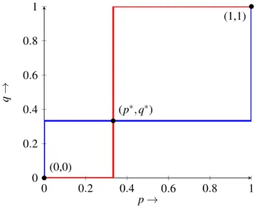
0 0.2 0.4 0.6 0.8 1 0 0.2 0.4 0.6 0.8 1 (p∗, q∗) (1,1) (0,0) p→ q →

Figure 1: Best response function

Let p and q denote the probability of player 1 and player 2 choosing action a respectively. Then the mixed Nash equilibrium corresponds to p = p∗and q = q∗ while the pure equilibria correspond to p= 0, q = 0 and p = 1, q = 1 respectively.

Also the utility at pure equilibrium (a, a) dominates the utility at the pure equilibrium (a, a) as ∆mi < 0 for (a, a) while ∆mi > 0 for (a, a).In the later section we will see that all the pure Nash equi-libria are ordered.

Thus, in general any n player game can have multiple Nash equilibrium. In the next section we describe a method to get a particular pure Nash equilibrium which we will later see is the best pure Nash equilibrium.

4

Iterative Method

In this section we describe a procedure to get a pure Nash equilibrium for every state m. We then show how two equilibria can differ from each other and the existence of ordering between the multiple Nash equilibria. For that we fix a state m and divide the players into 3 classes:

Class 1: Set of players for which Γi(m) > γiλi

∑j6=iλjaj and ∆

m

i > 0 irrespective of the action of other players

Class 2: Set of players for which Γi(m) < _∑γiλi

j6=iλjaj and ∆

m

players

Class 3: Set of players for which γiλi

∑j6=iλjaj < Γi(m) <

γiλi

∑j6=iλjaj. The optimal action depends on the

action of the other players as well.

Iterative Method

Step 1: Assign action a to players belonging to class 2 and 3 while action a to players of class 1. Step 2: Now, for all players in Class 3, calculate ∆m_i (a) using the current action sequence a. For players which have ∆m

i (a) > 0 assign them the new action a and place them in Class 1.

Step 3: Repeat Step 2 for the remaining set of players in Class 3 using the updated strategy, till we reach an equilibrium when no player in Class 3 has ∆m_i (a) > 0.

Note that (for m fixed) when a player i shifts to class 1, its action increases to a as ∆mi (a) > 0. But then ∆m_k(a) increases for all k 6= i. Hence through the iteration, ∆m_i is non-decreasing. As the number of players are finite and as ∆m

i is non-decreasing as the iteration moves forward, there is no need for the player to revert back to a. Thus, the equilibrium is bound to be reached. Now, every player with ∆m_i (a) > 0 has action a while every player with ∆m_i (a) < 0 has action a. Thus, no players has any reason to deviate from their current actions. Thus, we have reached a pure Nash equilibrium.

(Note: The way we have defined the iteration implies that the final action sequence will be unique.)

The game has the Finite Improvement Property (FIP) and thus has a generalized ordinal potential [3]. This property ensures that there always exists a pure Nash equilibrium.

Proposition: All the pure Nash equilibria in the game are ordered.

Proof: We assume there exist two Nash equilibria wherein neither is dominated by the other and then show that such an assumption leads to contradiction. To show this assume that the payoff for a player i at equilibrium is greater in one equilibrium (NE1) while the payoff for another player j is greater in the other (NE2).

Let us consider two equilibria u1and u2. Without loss of generality we may assume that they can be written as following (by renumbering the players). We have action vectors u1= (a1, .., an, b1, ..bK, c1..., cL) and u2= (a1.., an, b1’, ..., bK’, c1’, .., cL’) respectively. The actions aiare same in both equilibria, while the action sequence differ in the following way: bk= a and cl = a while bk’= a and cl’= a for all k and l. We will show that there cannot exist two such equilibria.

Consider two players i and j. For NE1we have bi= a and cj= a which means that ∆mi (u1) < 0 and ∆m

j(u1) > 0 respectively. While for the second equilibrium NE2we have bi’= a and cj’= a which gives us ∆mi (u2) > 0 and ∆mj(u2) < 0 . ⇒ ∆mj(u1) − ∆mj(u2) > 0 (4) ⇒ K

∑

∑

⇒ ∆mi (u2) − ∆mi (u1) > 0 (6) ⇒

_∑

∑

Adding the equations (5) and (7) we get

λi(a − a) + λj(a − a) > 0 (8)

This leads to contradiction and our assumption that such an equilibrium exists is false.

So, there cannot exist two equilibria in which the action of two players differ in the following way: in NE1ai= a, aj= a while in NE2 ai= a, aj = a. So, any two Nash equilibria will be of the form NE1= (a1, ..an, b1, ..bk) and NE2= (a1, ..an, b1’, ..bk’) where the action sequence aiare same in both cases while bi= a and bi’= a.

We now show NE1dominates NE2.

1. For players with action biit is obvious as ∆m_i in (2) changes sign from positive to negative and the utility increases.

2. Now, for the players with same action (ai) in both cases. The Numerator of the utility function (2) is a positive quantity.

The player can either have action a or a at a pure Nash equilibrium. In the first case the numerator of (2) is (M − m)λi while in the second case a∗= a which means ∆mi = −γi+ (M − m)λi> 0

and so is the numerator. Now, the denominator is smaller in NE1 (more players with action ai) than NE2which leads to an overall higher utility.

This concludes the proof.

We now claim that the Nash equilibrium obtained from the iterative process above gives the max-imum payoff and has no further refinement and that the optimal equilibrium strategy is threshold.

Proposition: The pure equilibrium obtained from the iterative method is the best equilibrium. Proof: Assume that there exists a refinement to the equilibrium from the proof above, i.e., there exists a Nash equilibrium where number of players with action a are greater than the number of players in the equilibrium generated by the iterative process. But if that were the case, then there would be a step during the iteration when this particular action sequence existed because we started with the base case of maximum number of players with action a . But if that action sequence were a Nash equilibrium then the iteration would stop.

So far we stated properties of equilibrium polies at a fixed state m. Next we study the dependence of the dominating equilibrium in m.

Proposition: The equilibrium strategy for player i at the best pure equilibrium is a threshold strategy.

Proof: Assume for a particular m∗the Nash action sequence is (a1, .., an) and that the a∗= ai, i.e, ∆m_i = (−γi+ (M − m∗)λi) ∑j6=iλjaj− λiγi> 0.

We have bi≥ ai∀i = 1 : N. → ∆m

i > ∆ m∗ i > 0.

So, ∀m such that m < m∗we have a∗_i = ai

Using similar arguments if for some m0, a∗i = aithen ∀m > m0we have a∗i = ai

Now, we present the closed form expression of the threshold for player i in terms of the parameters λi, γiand a. At threshold ∆mi ∗(a) = 0 ⇒ (−γi+ (M − m∗(i))λi) ∑j6=iλjaj− λiγi= 0 ⇒ −γi+ (M − m∗(i))λi= λiγi ∑j6=iλjaj ⇒ m∗(i) = M −γi λi− γi ∑j6=iλjaj

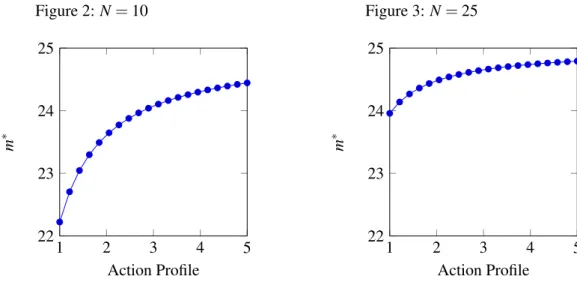
The threshold obtained might not always be an integer and in those cases, the least integer greater than m∗ acts as the threshold.In the figure below we show how the threshold m∗ changes with the action profile a−iof the other players.

Figure 2: N = 10 1 2 3 4 5 22 23 24 25 Action Profile m ∗ Figure 3: N = 25 1 2 3 4 5 22 23 24 25 Action Profile m ∗

Figure 4: Threshold m∗ versus action profile in a N player symmetric game.(M = 50,γ

λ = 25, a = 1, a = 5.)

In the special case where we have many players we can assume γiλi

∑j6=iλjaj → 0. and the expression

reduces to

⇒ m∗_{(i) = M −}γi

λi

(Note- Here the threshold only depends on the characteristics of player i which are known at the beginning of the game.)

For all m values greater than this threshold ∆mi < 0 and a∗i = a while for all m values lesser than threshold we have ∆m_i > 0 and a∗_i = a.

5

Conclusions and future directions

We have identified in this paper new structural properties of equilibria in stochastic games arising in competition over popularity in on-line social networks. Our starting point was the game described in [1]. We have discovered that there may be several pure equilibria and that when it is the case, then they are ordered in their performance. We have identified a procedure to obtain the equilibrium which is best for all players. We further showed the existence of a finite improvement property of the best response sequence and related this to the existence of a potential.

Although the competition model may seem to be restrictive, we show below that our model can describe more involved competition scenari. More precisely, we show how to handle competition models in which a destination does not limit itself to receive only a single content. Consider the case in which there is a Bernoulli trial with parameter q(i) that determines whether or not a destination that receives a content from i will still be interested to receive the next content. Instead of waiting an expo-nentially distributed time with parameter λi, a destination would wait an exponentially distributed time with parameter λ (i)q(i) (since the sum of a geometrically distributed number of i.i.d. exponentially distributed random variables is also exponentially distributed). We can thus handle this extension by simply using the initial model but with a scaled parameter of the exponential inter-opportunity times. As for future work, we notice that FIP implies the existence of a potential to our game, but its form is yet to be discovered.

References

[1] Eitan Altman, A stochastic game approach for competition over popularity in social networks, Dynamic Games and Applications, Springer Verlag, Vol. 3, No. 2 (2013) 313-323

[2] Eitan Altman, Constrained Markov Decision Processes,Chapman and Hall/CRC, 1999.

[3] Dov Monderer, Lloyd S. Shapley, Potential Games, Games And Economic Behaviour, Vol. 14, no. 1, may 1996, Pages 124-143