2D ICE TRAJECTORY IN THE FLOW FIELD OF
JOUKOWSKI AIRFOIL
by
Mahdi KAMOUSI ALAMDARI
THESIS PRESENTED TO ÉCOLE DE TECHNOLOGIE SUPÉRIEURE
IN PARTIAL FULFILLMENT FOR A MASTER’S DEGREE
WITH THESIS IN MECHANICAL ENGINEERING
M.A.Sc.
MONTREAL, MARCH 27, 2018
ÉCOLE DE TECHNOLOGIE SUPÉRIEURE
UNIVERSITÉ DU QUÉBEC
This Creative Commons license allows readers to download this work and share it with others as long as the author is credited. The content of this work can’t be modified in any way or used commercially.
BOARD OF EXAMINERS
THIS THESIS HAS BEEN EVALUATED BY THE FOLLOWING BOARD OF EXAMINERS
Mr. François Morency, Thesis Supervisor
Department of Mechanical Engineering, École de technologie supérieure
Mr. Stéphane Hallé, President of the Board of Examiners
Department of Mechanical Engineering, École de technologie supérieure
Mr. François Garnier, Member of the jury
Department of Mechanical Engineering, École de technologie supérieure
THIS THESIS WAS PRENSENTED AND DEFENDED
IN THE PRESENCE OF A BOARD OF EXAMINERS AND PUBLIC ON MARCH 22, 2018
ACKNOWLEDGEMENT
I would like to thank my thesis advisor Prof. François Morency at École de technologie supérieure. The door to Prof. Morency office was always open whenever I ran into a trouble spot or had a question about my research or writing. He consistently allowed this paper to be my own work, but steered me in the right direction whenever he thought I needed it.
I must express my very profound gratitude to my parents and to my family for providing me with unfailing support and continuous encouragement throughout my years of study and through the process of researching and writing this thesis. This accomplishment would not have been possible without them. Thank you.
TRAJECTOIRE 2D DE LA GLACE DANS UN ÉCOULEMENT
AUTOUR D’UN PROFIL DE JOUKOWSKI
Mahdi KAMOUSI ALAMDARI
RÉSUMÉ
Le givrage en vol et le dégivrage sont des problèmes important dans l'industrie de l'aviation et ont été étudié ces dernières décennies expérimentalement et numériquement. Au cours des dernières années, l'approche numérique a été privilégiée pour simuler la création de la glace et la trajectoire des pièces de glace en raison de son coût et de son efficacité temporelle. Cette étude vise à étudier l'influence des différents paramètres de la pièce de glace et du profil aérodynamique sur la probabilité d'ingestion de glace par un moteur monté à l'arrière d’un avion. Pour y parvenir, le profil d'écoulement de Joukowski et la trajectoire 2D d'une pièce de glace carrée dans ce champ d'écoulement seront étudiés.
Le champ de vitesse autour d’un profil de Joukowski est simulé et sera utilisé pour calculer les forces aérodynamiques sur la pièce de glace carrée. Les trajectoires des particules de glace en forme de plaques carrées dans des champs d'écoulement uniformes sont comparées à la littérature pour valider l’approche numérique. Comme le dégivrage est associé à des incertitudes sur les conditions initiales, la méthode de Monte-Carlo est utilisée pour faire une étude statistique sur le phénomène étudié. La probabilité de collision de glace autour du profil aérodynamique est calculée pour étudier l'influence des paramètres aérodynamiques tels que l'épaisseur, la courbure et l'angle d'attaque ainsi que l'influence de la forme et de la masse de la glace sur la trajectoire de la glace. Le dégivrage est étudié séparément pour l’intrados et l’extrados du bord d'attaque.
Les conditions initiales du dégivrage sont un facteur important dans les trajectoires de glace. Les résultats montrent que la probabilité d'ingestion de glace varie en fonction des paramètres de l'aile et de la pièce de glace. Les profils plus épais et plus incurvés imposent moins de risque d'ingestion de glace. L'angle d'attaque du profil aérodynamique a une influence différente sur la probabilité d’ingestion en fonction de l'emplacement du dégivrage. Les particules de glace rectangulaires et sphériques sont plus susceptibles de frapper le moteur que les morceaux de glace carrés. En outre, il est démontré que l'effet Magnus a une influence importante sur les trajectoires de la glace qui ne peut être ignorée dans les simulations.
Mots clés : CFD, trajectoire de la glace, profil de Joukowski, ingestion de glace, givrage en
2D ICE TRAJECTORY IN THE FLOW FIELD OF THE JOUKOWSKI
AIRFOIL
Mahdi KAMOUSI ALAMDARI
ABSTRACT
Inflight icing and ice shedding as an important problem in the aviation industry have been studying in recent decades both experimentally and numerically. In recent years, the numerical approach has been privileged to simulate ice accretion and ice piece trajectory due to its cost and time efficiency. This study aims to investigate the influence of the different characters of the ice piece and airfoil on the probability of ice ingestion by an aft-mounted engine. In this order, the flow field of the Joukowski airfoil and 2D trajectory of a square plate ice piece in this flow field will be simulated.
Velocity field of Joukowski airfoil is simulated and used to compute aerodynamic forces on the square plate ice piece. Trajectories for square plate ice particles in uniform flow fields are compared with the literature to validate the developed code. As the ice shedding is associated with uncertainties regarding its initial conditions, Monte-Carlo method is used to have a statistical study on this phenomenon. Ice pass probability map around the airfoil is generated to investigate the influence of airfoils’ parameters such as thickness, camber and angle of attack as well as the influence of ice’s shape and mass on the trajectory of the ice piece. Ice shedding is investigated separately for upside and downside of the leading edge.
Initial condition of ice shedding is found to be an important factor in ice trajectories. Results show that ice ingestion probability by engine changes for different set of parameters of airfoil and ice piece. Thicker and more curved airfoils impose less ice ingestion risk. Airfoil’s angle of attack has different influence on the probability map depending on the location of the ice shedding. Rectangular and sphere ice particles are more likely than square ice pieces to pass through the engine. Also it is shown that Magnus effect has an important influence on the ice trajectories which cannot be ignored in ice trajectory simulations.
TABLE OF CONTENTS
Page
INTRODUCTION ... 1
CHAPTER 1 LITRATURE REVIEW... 5
1.1 In-flight icing and engine of aircraft ... 5
1.2 Ice trajectory simulation ... 9
1.3 Contributions ... 13
CHAPTER 2 MATHEMARICHAL MODEL AND SIMULATION METHODOLOGY .. 15
2.1 Flow fields ... 15
2.1.1 Flow field around the circular cylinder ... 15
2.1.1.1 Uniform, doublet and vortex flow fields ... 16
2.1.1.2 Superposition of the flow fields ... 18
2.1.1.3 Joukowski transformation ... 19
2.1.2 Joukowski airfoil and its flow field ... 21
2.1.2.1 Parameters to design a Joukowski airfoil ... 21
2.2 Two dimensional ice particle trajectory simulation model ... 26
2.2.1 Relative velocity of the ice piece and its orientation ... 26
2.2.2 2D force components on the ice piece ... 28
2.2.3 Ice piece’s angle of attack : ... 30
2.2.4 Lift, drag and moment coefficients ... 31
2.2.5 Magnus effect ... 33
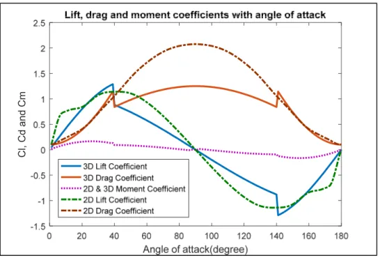
2.2.6 2D lift, drag and moment coefficients ... 35
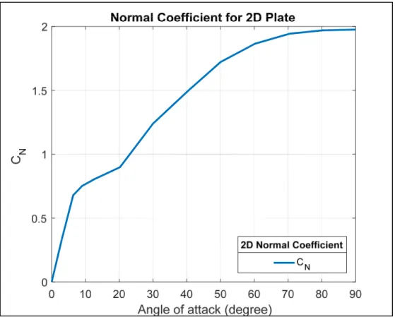
2.2.7 Coefficients for Sphere ice piece ... 38
2.2.8 2D differential equations of motion ... 39
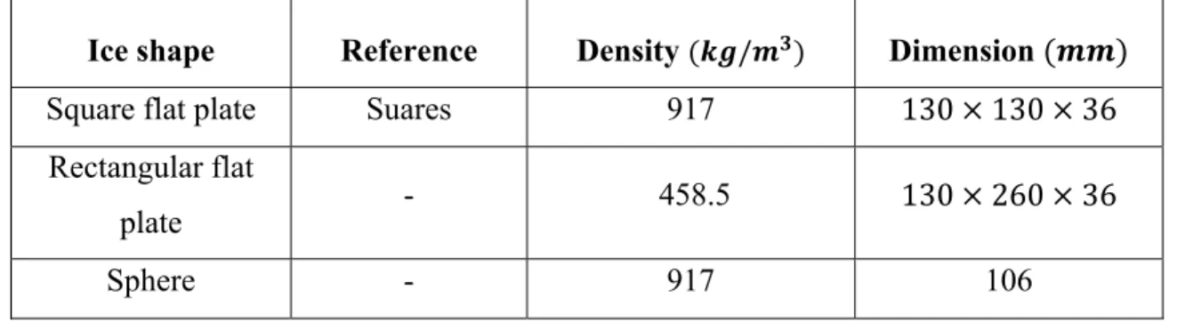
2.2.9 Ice piece samples and their properties ... 41
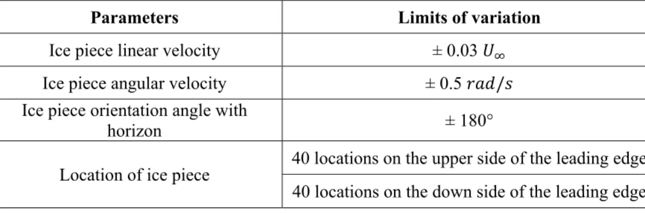
2.3 Monte-Carlo statistical study ... 43
CHAPTER 3 RESULTS AND DISCUSSION ... 49
3.1 Joukowski airfoil ... 49
xii
3.1.2 Center of the circle in different quadrants ... 51
3.1.3 Thickness of the airfoil and lift force ... 53
3.1.4 Camber of the airfoil and lift force ... 54
3.1.5 Airfil’s angel of attack and lift force ... 56
3.2 2D ice trajectory in horizontal uniform flow field ... 58
3.2.1 Trajectories without Magnus effect ... 58
3.2.2 Trajectories with Magnus effect ... 61
3.3 2D Ice trajectory in Non-horizontal uniform flow ... 65
3.4 2D ice trajectory in Joukowski airfoil’s flow field ... 67
3.4.1 Airfoil’s angle of attack and trajectories ... 71
3.4.2 Airfoil’s thickness and trajectories ... 73
3.4.3 Airfoil’s camber and trajectories ... 74
3.4.4 Flight altitude and trajectories ... 75
3.5 Monte-Carlo simulations ... 77
3.5.1 Effect of the airfoil’s angle of attack on the probability map ... 78
3.5.2 Effect of the thickness of the airfoil on the probability map ... 84
3.5.3 Effect of the camber of the airfoil on the probability map ... 88
3.5.4 Effect of the ice piece’s size on the probability map ... 91
3.5.5 Effect of the Magnus coefficients on the probability map ... 94
3.5.6 Effect of the ice shape on the probability map ... 97
3.5.7 Effect of the normal random initial conditions on the probability map ... 103
CONCLUSIONS AND RECOMENDATIONS ... 111
LIST OF TABLES
Page
Table 2.1 Properties of the square plate ice pieces used in our simulations ... 42 Table 2.2 Properties of the sample ice particles used in Monte-Carlo simulations ... 43 Table 2.3 Variation of initial parameters for square plate ice piece trajectories around the
LIST OF FIGURES
Page
Figure 2.1 Joukowski transformation... 20
Figure 2.2 Angle of the relative velocity (α) ... 27
Figure 2.3 Force components on the ice piece ... 28
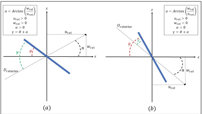
Figure 2.4 The angle between the relative velocity and the ice piece (γ) ... 31
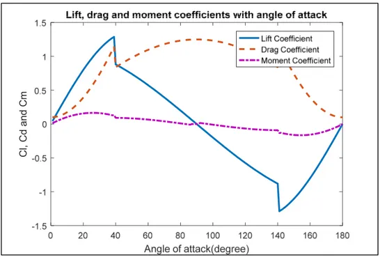
Figure 2.5 Lift, drag and moment coefficients ... 33
Figure 2.6 2D & 3D lift, drag and moment coefficients and angles of attack ... 36
Figure 2.7 Normal coefficient for the 2D rectangular ... 37
Figure 2.8 Square plate ice piece and its dimension ... 41
Figure 2.9 The dimension of the sphere and rectangular ice particles ... 43
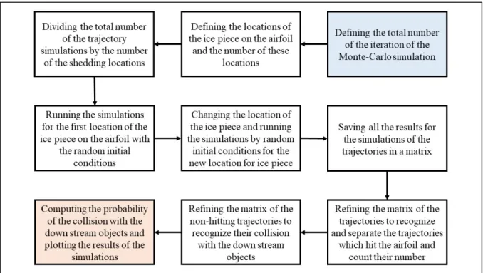
Figure 2.10 Diagram of the Matlab code for Monte-Carlo simulations ... 48
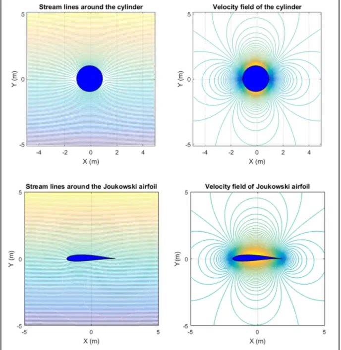
Figure 3.1 Graphical results of the Joukowski airfoil Matlab code ... 50
Figure 3.2 Joukowski airfoil with the center of the cylinder in the different quadrants of plane ζ 51 Figure 3.3 Comparison between the results of our Matlab code (left) and the results of Newman (right), up: Joukowski airfoil and stream lines, down: velocity field ... 52
xvi
Figure 3.5 Four Joukowski airfoils with different cambers, up-left: ζ0 = −0.1 + 0.000001i, up-right: ζ0 = −0.1 + 0.02i, down-left: ζ0 = −0.1 + 0.04i, down-right: ζ0 = −0.1 + 0.06i, the radius of the circle is R = 1 m. ... 55 Figure 3.6 Joukowski airfoil with different angles of attack ... 57 Figure 3.7 Comparison of trajectories between Holmes’s results and computed trajectories -
square plastic plate (40 × 40 × 2 mm) with a density of 1163 kg/m3 ... 59 Figure 3.8 Comparison of trajectories between Holmes’s results and computed trajectories -
square basswood plate (75 × 75 × 9 mm) ... 60 Figure 3.9 Comparison of trajectories between Holmes’s results and computed trajectories
with Magnus effect- plywood square plate (75 × 75 × 3 ) with a density of
847 / 3 ... 62 Figure 3.10 Comparison of the trajectories between Kordi’s results and computed trajectories
with Magnus effect - square plastic plate (40 × 40 × 2 ) with a density of
1120 / 3 ... 63 Figure 3.11 Comparison of trajectories and Velocities between Kordi’s results and computed
trajectories with Magnus effect- basswood square plate (75 × 75 × 9 mm) with a density of 575 kg/m3 ... 64 Figure 3.12 Comparison of trajectories in non-horizontal uniform flow field with different
angle of the flow with the horizontal axis - Magnus effect included – up: plastic square plate (40 × 40 × 2 mm) with a density of 1120 kg/m3 - down: square basswood plate (75 × 75 × 9 mm) with a density of 575 kg/m3, ρair = 1.24 kg/m3. ... 66 Figure 3.13 Comparison of the trajectories in a uniform flow field without Magnus effect –
square plate ice piece with a dimension of 0.1303 m × 0.1303 m × 0.0365 m and a mass of 0.5715 kg. ... 68 Figure 3.14 Comparison of the trajectories in the flow field of two airfoils (Joukowski airfoil
and NACA 23012) without Magnus effect- square plate ice piece with a dimension of 0.1303 m × 0.1303 m × 0.0365 m and a mass of 0.5715 kg. ... 70
xvii
Figure 3.15 Comparison of the trajectories in the flow field of Joukowski airfoil with different angle of attacks for the airfoil without Magnus effect - square plate ice piece with a dimension of 0.1303 m × 0.1303 m × 0.0365 m and a mass of 0.5715 kg. ... 72 Figure 3.16 Comparison of the trajectories in the flow field of Joukowski airfoils with different
thicknesses without Magnus effect - square plate ice piece with a dimension of
0.1303 m × 0.1303 m × 0.0365 m and a mass of 0.5715 kg. ... 73 Figure 3.17 Comparison of the trajectories in the flow field of Joukowski airfoils with different
cambers without Magnus effect - square plate ice piece with a dimension of
0.1303 m × 0.1303 m × 0.0365 m and a mass of 0.5715 kg. ... 75 Figure 3.18 Comparison of the trajectories in the flow field of Joukowski airfoil in different
altitudes (different air densities) - square plate ice piece with a dimension of
0.1303 m × 0.1303 m × 0.0365 m and a mass of 0.5715 kg. ... 76 Figure 3.19 Monte-Carlo simulation for square plate ice around the Joukowski airfoil with
AOA=0° (left) and AOA= 4° (right), Ice particle 13 × 13 × 3.6 mm, mice = 0.5715 kg, ρair = 0.770 kg/m3, shedding is from the upside surface of the leading edge, Magnus effect included. ... 79 Figure 3.20 Monte-Carlo simulation for square plate ice around the Joukowski airfoil with
AOA=0° (left) and AOA= 4° (right), Ice particle 13 × 13 × 3.6 mm, mice = 0.5715 kg, ρair = 0.770 kg/m3, Shedding is from the downside surface of the leading edge, Magnus effect included. ... 80 Figure 3.21 Monte-Carlo simulation for square plate ice around the Joukowski airfoil with
AOA=0° (left) and AOA=15° (right), Ice particle 13 × 13 × 3.6 mm, mice = 0.5715 kg, ρair = 0.770 kg/m3, shedding is from the upside surface of the leading edge, Magnus effect included. ... 81 Figure 3.22 Monte-Carlo simulation for square plate ice around the Joukowski airfoil with
AOA=0° (left) and AOA=15° (right), Ice particle is 13 × 13 × 3.6 mm and mice = 0.5715, ρair = 0.770 kg/m3, Shedding is from the downside surface of the leading edge, Magnus effect included. ... 82 Figure 3.23 Comparison between the results of Suares for trajectories with different angle of
xviii
Figure 3.24 Monte-Carlo simulation for square plate ice around the Joukowski airfoil with thickness t/c= 13% (left) and thickness t/c=6.5% (right), Ice particle is 13 × 13 × 3.6 mm and mice = 0.5715, ρair = 0.770 kg/m3, shedding is from the upside surface of the leading edge, Magnus effect included. ... 86 Figure 3.25 Monte-Carlo simulation for square plate ice around the Joukowski airfoil with
thickness t/c= 13% (left) and thickness t/c=6.5% (right), Ice particle is 13 × 13 × 3.6 mm and mice = 0.5715, ρair = 0.770 kg/m3, shedding is from the downside surface of the leading edge, Magnus effect included. ... 87 Figure 3.26 Monte-Carlo simulation for square plate ice around the curved (left) and symmetric
(right) Joukowski airfoil), Ice particle is 13 × 13 × 3.6 mm and mice = 0.5715, ρair = 0.770 kg/m3, shedding is from the upside surface of the leading edge, Magnus effect included. ... 89 Figure 3.27 Monte-Carlo simulation for square plate ice around the curved (left) and symmetric
(right) Joukowski airfoil), Ice particle is 13 × 13 × 3.6 mm and mice = 0.5715, ρair = 0.770 kg/m3, shedding is from the downside surface of the leading edge, Magnus effect included. ... 90 Figure 3.28 Monte-Carlo simulation for different square plate ice around the Joukowski airfoil),
left: Ice particle 13 × 13 × 3.6 mm and mice = 0.5715, right: Ice particle 6.5 × 6.5 × 1.8 mm and mice = 0.2857, ρair = 0.770 kg/m3, shedding is from the upside surface of the leading edge, Magnus effect included. ... 92 Figure 3.29 Monte-Carlo simulation for different square plate ice around the Joukowski airfoil),
left: Ice particle 13 × 13 × 3.6 mm and mice = 0.5715, right: Ice particle 6.5 × 6.5 × 1.8 mm and mice = 0.2857, ρair = 0.770 kg/m3, shedding is from the
downside surface of the leading edge, Magnus effect included. ... 93 Figure 3.30 Monte-Carlo simulation for square plate ice around the Joukowski airfoil with (left)
and without (right) Magnus effect, Ice particle 13 × 13 × 3.6 mm, mice =
0.5715 kg, ρair = 0.770 kg/m3, shedding is from the upside surface of the leading edge. ... 95 Figure 3.31 Monte-Carlo simulation for square plate ice around the Joukowski airfoil with (left)
and without (right) Magnus effect, Ice particle 13 × 13 × 3.6 mm, mice =
0.5715 kg, ρair = 0.770 kg/m3, shedding is from the downside surface of the leading edge ... 96
xix
Figure 3.32 Monte-Carlo simulation for sphere ice piece around the Joukowski airfoil, shedding from upside (left) and downside (right) surface of leading edge, Ice particle D =
106 mm, mice = 0.5715 kg, ρair = 0.770 kg/m3 ... 98 Figure 3.33 Monte-Carlo simulation for square (left) and rectangular ice piece (right) around the
Joukowski airfoil, shedding is from upside surface of the leading edge, rectangular ice; 130 × 260 × 36 mm, mice = 0.5715 kg, ρair = 0.770 kg/m3, Magnus effect included ... 100 Figure 3.34 Monte-Carlo simulation for square (left) and rectangular ice piece (right) around the
Joukowski airfoil, shedding is from downside surface of the leading edge, Ice particle 130 × 260 × 36 , = 0.5715 , = 0.770 / 3, Magnus effect included ... 101 Figure 3.35 Comparison with the results of Suares for trajectories of rectangular ice plate ... 102 Figure 3.36 Comparison of the Monte-Carlo simulations for square and rectangular ice plates ... 103
Figure 3.37 Comparison of Monte-Carlo simulation with uniform and normal random numbers , shedding is from upside surface of the leading edge, Ice particle 130 × 130 × 36 mm, mice = 0.5715 kg, ρair = 0.770 kg/m3, Magnus effect included ... 105 Figure 3.38 Comparison of Monte-Carlo simulation with uniform and normal random numbers ,
shedding is from downside surface of the leading edge, Ice particle 130 × 130 ×
36 mm, mice = 0.5715 kg, ρair = 0.770 kg/m3, Magnus effect included ... 106 Figure 3.39 Comparison of Monte-Carlo simulation with uniform and normal random numbers,
shedding is from upside surface of the leading edge, Ice particle 130 × 130 ×
36 mm, mice = 0.5715 kg, ρair = 0.770 kg/m3, Magnus effect included ... 108 Figure 3.40 Comparison of Monte-Carlo simulation with uniform and normal random numbers ,
shedding is from downside surface of the leading edge, Ice particle 130 × 130 ×
LIST OF SYMBOLS Mathematical symbols: Lift Coefficient Drag Coefficient Moment coefficient Flow velocity
Vertical component of the flow velocity Horizontal component of the flow velocity Horizontal velocity component of the ice particle Horizontal velocity component of the ice particle Angle of the relative velocity with horizontal axis Angle of attack of the ice particle
Normal force coefficient Drag force on the ice particle Lift force on the ice particle Moment on the ice particle Gravity acceleration
Moment of inertia on the ice particle Mass of the ice particle
Normal force on the ice particle Reference area of the ice particle time
Angle of the circles offset Density
Angular velocity
Length of the ice particle Width of the ice particle
xxii
Thickness of the ice particle
Distance of the pressure center with the center of ice
Drag coefficient caused by Magnus effect Lift Coefficient caused by Magnus effect Moment coefficient caused by Magnus effect
The Plane of the Joukowski airfoil The plane of the circular cylinder
Units:
Meter, unit of length . Feet, unit of length
/ Meter per second, unit of velocity
/ Kilogram per cubic meter, unit of density Second, unit of time
° Degree, unit of angle
° Degree Celsius , unit of temperature
Abbreviations:
2D Two-Dimensional 3D Three-Dimensional AOA Angle of Attack
CFD Computational Fluid Dynamic LWC Liquid Water Content
NACA National advisory Committee for Aeronautics DOF Degree of Freedom
TWC Total Water Content
INTRODUCTION
Ice accretion on aircraft is one of the hazardous phenomena that can cause catastrophic accidents. This issue has been under investigation for several decades and especially in recent years to solve the problems related to icing and ice shading in the aviation industry. Although many empirical and computational methods have been implemented, but icing problem still remains as an important threat to aircraft safety and efficiency. Icing during the flight brings about degradation of the aircraft’s performance and shading of the accreted ice can damage the downstream components of an aircraft such as engines.
In recent years, Computational Fluid Dynamic (CFD) has been considered as a privileged approach to study icing and ice shedding phenomenon. Due to the efficiency of this method regarding time and cost, CFD models have been widely used to predict the ice accretion on the component of the aircraft such as leading edges, control surfaces and engine nacelles. Also this numerical approach is used to study the trajectory of the ice particles shed from the geometry of the aircraft (Shimoi, 2010) (Suares, 2005).
Ice trajectory simulations have been carried out to trace the path of the shed ices and compute the ice pass probability and their strike with the component of the aircraft. Studies concern both two-dimensional and three-dimensional movement of the ice mass. While in the majority of the 2D simulation, the ice piece has three Degrees of Freedom (DOF) of movement, in 3D simulations DOF vary from three to six. The flow fields used in the simulations can be uniform or non-uniform. The uniform flow field can be a representative of the wind tunnel flow and the non-uniform flow fields can be the flow field of airfoil, wing or an aircraft as a whole. The shape of the ice fragment plays an important role in ice trajectory results. Aerodynamic force and moment coefficients, which are mostly calculated through empirical methods, differ for each shape of the ice piece. Although the shape of shed ice pieces is random, simulations are conducted for some ice shapes such as square plates, rectangular plats, spheres, semi sphere and disk shape ice shapes (Shimoi, 2010).
2
The ice piece moves in a flow field due to the imposed forces and moments. Both aerodynamic and gravitational forces govern the acceleration of the ice mass. While the forces translate the ice piece in the flow filed, moments are in charge of the angular movement of the particle. In some research all the forces and moments are taken into account and some others have limited their studies by neglecting some of the aerodynamic forces such as Magnus effect, generated by the angular velocity of the ice piece.
This research project will consider the trajectory of a square plate ice in a two-dimensional flow field. DOF for the ice piece will be three for two linear movements in the directions of the horizontal and vertical axis of the plane and an angular movement around the axis perpendicular to the plane of the 2D flow field. Lift and drag forces as well as the moment on the ice piece will be calculated using both the static aerodynamic coefficients and the aerodynamic coefficients generated by the angular velocity of the ice particle (Magnus effect). The flow fields used in this research project are uniform and non-uniform flow fields. The trajectories run in the uniform flow field will serve for validation of the simulation code and non-uniform flow field will be used to draw the results of the research. Joukowski airfoil is the geometry which the flow field around it will be simulated.
Ice trajectory will be simulated in a 2D flow field using differential equation of the movement. The velocity and the position of the ice piece will be computed by integrating these differential equations in each time step of the trajectory. Aerodynamic and gravitational forces will be used to obtain the linear acceleration of the ice body and moment of inertia will be used to compute angular acceleration of the ice fragment.
The random nature of the ice shedding makes the statistical study inevitable for this phenomenon (Suares, 2005), (Shimoi, 2010). The initial condition of the ice shedding is associated with uncertainties regarding ice piece’s shape, location, orientation and linear and initial angular velocities. A code developed for Monte-Carlo method will be integrated with the code of ice trajectory. This code generates a large number of initial conditions and plot the footprint of the ice pieces around the airfoil. Using this integrated code, the probability of the ice trajectory through the defined areas in the study plane will be possible.
3 This research will be presented in three chapters. First chapter will deal with the background of the icing problem and ice trajectory simulation. First comes an introduction for in-flight icing problems. The meteorological conditions in which the probability of in-flight icing is higher and the process of ice accretion on the components of the aircraft, in particular inside the engine, will be presented. The possible approaches to analyze icing problems and currently used de-icing systems in the aviation will be mentioned briefly. These sections will be followed by a literature review related to the ice trajectory simulation methods.
Chapter two is dedicated to the methodology of the research project. it will offer the mathematical model, equations and coefficients used in the simulation code. In addition, the condition of the flow fields and properties of ice particles simulated in the research will be mentioned. In another section, the simulation tools used in the project will be described by illustrating the flow chart of the Matlab codes developed during the research.
Chapter three contains the results of the research project. The results will be validated, verified and discussed for Joukowski airfoil, single trajectories and Monte-Carlo method. The figures generated by the simulation code will show the probability maps around the airfoil in different situations. This chapter will discuss the impact of the airfoil’s angle of attack, airfoil thickness and its camber on the trajectory of the ice piece. Also, the possibility of the ice ingestion by downstream engines will be verified when the ice piece has different shapes such as square, rectangular and sphere shape and different masses.
CHAPTER 1 LITERATURE REVIEW
1.1 In-flight icing and the engine of aircraft
According to Bin and Yanpei (Bin and Yanpei, 2011), the source of the ice accreted on the propulsion system can be different, but usually, engine icing is caused by freezing of cloud droplets, or super cooled water droplets. Super cooled water droplets maintain their liquid state even at temperatures well below the freezing degree. When these droplets impinge on the aircraft’s engine during the flight, they can bring about anomalies such as non-recoverable or repeating surge, stall rollback or flameout, and may also cause the gas path ice blockage in core engine (Bin and Yanpei, 2011).
The presence of high altitude ice crystals which exist in the deep convective clouds of strong tropical and sub-tropical storms is known to be the other causation of this problem. These ice crystals do not have good reflectivity for radar echoes, so it is difficult to prevent passage of aircraft through these clouds (Califf and Knezevici, 2014). According to Haggerty, McDonough et al. (Haggerty, McDonough et al., 2012), several aeronautic accidents which are attributed to engine icing, have occurred in flight conditions where super cooled liquid droplets were not present. In these cases, ice crystal particles in surrounding clouds are considered to have the main role in degradation of engine power. Since the mid-1990’s, more than 100 documented engine power loss events are attributed to this phenomenon known as ice particle icing. The majority of accidents related to ice particle icing phenomenon, have occurred in the vicinity of tropical thunderstorms, particularly over the western tropical Pacific Ocean. It is hypothesized that ice particles accrete on warm surfaces inside the engine. These Ice masses deform the aerodynamic shape of the blades and may block the airflow passage inside the engine. Also, accreted ices can shed into the engine which is hazardous for downstream components. All these factors reduce performance of the engine dramatically (Haggerty, McDonough et al., 2012).
6
Veres, Jorgenson et al. (Veres, Jorgenson et al., 2012) estimate that ingested ice crystals into the engine will confront with higher temperatures in core part of the engine. This condition will melt a portion of the ice crystals. It will make a mixture of ice and water which consequently enhances the stickiness power of ice particles on the metal surfaces of the compressor components. Thus, the engine experiences airflow blockage on its stationary parts such as stator vanes (Veres, Jorgenson et al., 2012).
According to Veres, Jorgenson et al. (Veres, Jorgenson et al. 2012), local wet-bulb temperature and minimum local melt ratio are two key parameters that play main roles to provide favorable condition for ice accretion. It is known that this favorable condition takes place when the local wet-bulb temperature is near and blow freezing and the local melt ratio is 10%. These criteria can be used to determine the possibility of icing due to ice crystals. The degree of ice blockage can be estimated by using an empirical model of ice growth rate and the impingement duration of ice crystals (Veres, Jorgenson et al. 2012).
Liquid water content (LWC), total water content (TWC), flight Mach number, particle impingement angle and particle size are the factors that determine the sticking efficiency of ice crystals particles (Currie, Fuleki et al., 2014). A former research (Currie, Fuleki et al., 2014) suggests that the sticking efficiency remains finite at all particle impingement angles when TWC is more than 10 / and the flight Mach number is low (0.25). At higher Mach numbers, smaller ice crystal particles stick more efficiently to engine components.
Over the past decades, aircraft flight accidents related to icing has been reported all over the world. According to Cao, Wu et al. (Cao, Wu et al., 2015), in America, statistic data of flight accidents during 1973 to 1977 showed that 2.56% of the total flight accidents are due to the icing problem. During 1976 and 1988, flight accidents attributed to ice accretion reached up to 542. American Safety Advisor statistic data concerning iced- aircraft flight accidents from 1990 to 2000 indicates that 12% of all the flight accidents in adverse weather conditions occurred in icing condition and in-flight icing was the reason for 92% of the iced-induced accidents (Cao, Wu et al., 2015).
7 Since 1990, many of jet engine power loss incidents have been attributed to the icing problem, which have been occurred at altitude higher than 22,000 ft., the level which is recognized as the extreme upper limit for the existence of super cooled liquid water (Mason, Strapp et al., 2006). Mason, Strapp et al estimate that at this level the hydrometeors are expected to exist in the form of ice particles which can be individual ice crystals or in larger size spanning from microns to centimeters. Previous to these events, it was believed that ice particles are harmless for the airframe and the engine due to the fact that frozen particles don’t stick to these components and bounce off from the surface. Recent engine power loss events since 1990, initiated deeper investigation of ice particles influence on jet engines. More than 240 icing related events have been documented worldwide since the 90s, which 62 of them are believed to be due to ice particle icing (Mason, Strapp et al., 2006).
According to Mason, Strapp et al. (Mason, Strapp et al., 2006), documented icing incidents and accidents show that most of the ice crystal icing occurs during aircraft flights through convective clouds. Convective clouds have updraft cores that cause the movement of low-level air to higher altitudes in which the temperature drops and water vapor condense continuously. This phenomenon can increase the liquid water content (LWC) and/or ice water content (IWC) in a limited region. It is assumed that condensing vapor goes directly to the ice phase above the freezing level. The maximum level of IWC is about 9 g/m3 at 30,000 ft. and as the altitude
increases above this level, IWC decreases. Previous observations show that Atlantic hurricane convection clouds are almost completely glaciated at -5°C which means rapid conversion of LWC to ice above the freezing level and no significant super cold LWC exist at temperature below -12°C (Mason, Strapp et al., 2006).
The accreted ice on the aircraft’s surfaces can be in two general forms. These forms are called glaze ice and rime ice. As Borigo (Borigo, 2014) describes, glaze ice is a clean and hard ice that usually does not have an aerodynamic shape. When droplets do not freeze instantaneously and run downstream the result will be a glaze ice accretion. Because of its non-aerodynamic shape, it is more vulnerable to shedding. The creation of rime ice is very fast and as soon as droplets impinge with the surface, freezing occurs and ice traps some air which makes it milky and white. Rime ice has greater adhesion properties and lower density (Bin and Yanpei, 2011).
8
Rime ice usually grows in low temperature (-40°C to -10°C) at lower speeds and at low LWC conditions but glaze ice typically accretes at temperatures closer to freezing (-18°C to 0°C) at higher speeds and LWC (Borigo, 2014).
An engine of aircraft should pass icing test to get its certification. An engine should be able to work steadily without any problem under a specific icing condition (Bin and Yanpei, 2011). These requirements are mentioned in FAR Section 33.68. This Section requires that each engine which is equipped with ice protection system should be able to sustain its power during flight phases without ice accretion on components and run steadily under icing condition at least for 30 minutes at ground idle setting and then demonstrate its takeoff thrust by being able to accelerate without any problem. This performance requirement is defined in appendix C of FAR part 25. Engine does not use its auto-recovery system during icing test, since it is a back-up device for aircraft during the icing problem (Bin and Yanpei, 2011).
Icing can be analyzed both experimentally and numerically. The experimental approach to analyze icing can be done during a real flight or in the wind tunnel. Both of these approaches are suitable to analyze a system, but they cannot be used in the design platform (Pellissier, 2010). Testing an aircraft during a real flight would be very expensive and it can be used just after production of the aircraft. This method is time consuming and finding an icing condition in flight to examine the performance of the engine is very difficult. Inflight-testing is dangerous and difficult to run and all the icing conditions outlined in aviation safety regulation such as the FAA’s FAR (Federal Airworthiness Regulations) Part 25 Appendix C or the EASA’s CS (Certification Specifications) Part 25 Appendix C cannot be reproduced (Pellissier, 2010). Using wind-tunnel can be a solution for problems associated with in flight testing but it has its own limitations. Icing test facilities utilize freezing super cooled droplets or ice shavers to simulate icing condition. There are differences between an artificial ice crystal produced in icing wind tunnel and a natural ice crystal which can be found at high altitude. Since the shape of the crystal is a key element to study the trajectory of ice particles, such inadequate simulation of ice crystals misleads the analyses of the icing dynamics (Nilamdeen, 2010). The number of icing wind tunnels is very limited and manufacturers own most of the wind tunnels, so there are few facilities in research domain that are accessible for researchers. The price of using
9 these wind tunnels is expensive and even ignoring the cost will not help much due to the fact that most of the good facilities that can produce icing condition are booked in advance for a long time.
Beside the experimental methods, computational models are used to compute ice accretion, evaluate the performance degradation caused by icing, study and design anti-icing systems and evaluate their efficiency. According to Rios (Rios Pabon, 2012), the complicity of analyzing the ice crystal trajectory and the problems of experimental approach favor the use of computational methods. By using these methods ice shape and its trajectory can be simulated more efficiently. The time and money needed to run these analyzes are significantly less than experimental methods.
1.2 Ice trajectory simulation
A literature review was conducted to establish the state of the art in the fields related to ice shedding and ice piece trajectory simulation. This literature review concerned the ice trajectory simulation methods and the probabilistic methods for numerical studies on this phenomenon. Following is the results of a literature review which introduces works done in the ice trajectory simulation.The ice trajectory simulation as a numerical tool to investigate the inflight icing and ice shedding has been considered and developed in recent decades and there are not many available papers and data in the literature. Most of the works done to simulate the trajectories are in the field of wind engineering and to simulate the trajectories of the debris in the storms (Tachikawa, 1983), (Kordi, 2009), (Holmes, 2006). However, some researchers have applied this knowledge in the field of ice shedding problem and ice piece trajectories (Shimoi, 2010), (Suares, 2005).
This research has been done with different considerations. Two general categories in the ice piece trajectory simulations are the trajectories which are simulated in 2D flow fields and the trajectories which are carried out in 3D flow fields. Moreover, the degree of freedom of the movement of the ice piece is confined in the research and can vary from 2 DOF to 6 DOF.
10
The flow fields in which ice trajectories are studied are divided to uniform and non-uniform flow fields. The trajectories in the uniform flow field are mostly used to validate the data of the simulations with the experimental data and results of the wind tunnel experiments. The non-uniform flow fields used in the simulations are the flow field of the aircraft’s geometry as a whole or the flow field of components of the aircraft such a wing.
Tachikawa (Tachikawa, 1983) is a pioneer researcher in the field of the trajectory simulation. He has carried out several 2D experiments in the wind tunnel to determine the aerodynamic force coefficients on the different shape of the plates. He has measured the lift and drag forces and moments on the plate in a low-speed wind tunnel. Magnus effect is taken into account to simulate the trajectories and the results are compared with the experimental trajectories with different initial conditions for different plates. In his research he has shown that the initial orientation of the plate plays an important rule to determine the path of the plate.
Holmes et al. (Holmes, 2006) has conducted plate type debris trajectory simulation in 2D uniform flow field experimentally and numerically. He has investigated the trajectory of three different square flat plate debris with different dimensions and density in the uniform horizontal flow fields with different velocities. The differential equations of movement are used to calculate the trajectory of the debris. He has used aerodynamic force coefficients which are a function of the angle of attack, to calculate the lift, drag and moment forces on the plate. The Magnus effect in the simulation of Holmes is only considered for lift force and he has compared the trajectories with and without Magnus effect. Holmes has compared their trajectories with experimental data of Texas Tech University. In the article of Holmes there are some examples of trajectories for different plate pieces with different initial conditions for the angle of attack of the ice piece and its initial velocity to compare the influence of the initial conditions on the trajectories of the plate debris.
Kordi and Kopp (Kordi, 2009) have simulated the trajectory of the square flat plate in 2D uniform flow field. They have used differential equations of motion to trace the movement of the ice particle. The aerodynamic coefficients generated by the angular velocity of the ice piece are added to the static coefficients to take into account the Magnus effect, in this order, the
11 equations of Iverson (Iverson, 1979) are used based on the ice piece’s tip speed and the speed of the tip of the auto rotational point.
Suares (Suares, 2005) has performed a broad research on the trajectory simulation of ice pieces in uniform and non-uniform flow field. He has simulated the ice trajectory in 2D and 3D for uniform flow and flow fields of the airfoil and wing. The ice piece samples used in the trajectories are square plates, rectangular plates and semicircular shells and the research includes 3,4 and 6 degrees of freedom for the movement of the ice piece samples. Suares has developed codes in FORTRAN and MSC.Easy5 for ice trajectory simulation and by using Monte-Carlo method the strike possibility of the ice piece with downstream engines in different conditions has been studied.
Chandrasekharan and Histion (Chandrasekharan, 2003) have simulated the trajectory of the ice pieces shed from the surface of the aircraft to analyze the probability of the ice ingestion by downstream engines when the minor modifications are made in the dimension of the fuselage. The VSAERO code has been utilized to compute the flow field and velocity field around the geometry of the Learjet 40 and Learjet 45 business jets. In the simulation, the lift and side forces on the ice particle have been dismissed and the movement of the ice fragment and its acceleration in the flow field is calculated only using the drag forces and gravitational forces. The project includes the simulations of disk and plate shape ice pieces. The disk ice particle has a diameter of four inches and a thickness of one inch and start its shedding from the radome of the aircraft. Two plate form ice pieces with dimensions of 3" × 1" × 1" and 1.5"×1.5" × 0.3" are used to simulate the ice shedding from the windshield of the aircraft. The obtained results show that the minor different in the length of two above mentioned aircraft does not have a significant influence on the ice ingestion risk of the downstream engines.
A 4-DOF simulation model has been used by Kohlman and Winn (Kohlman, 2001) to simulate the square plate ice trajectories in the uniform flow field. Lift and drag forces are assumed to be the main forces on the ice fragment and experimental data have been used to calculate the aerodynamic coefficients. The forces generated by the rotation of the ice piece are taken into account by calculating the angular velocity, aerodynamic damping and moment of inertia for
12
the plate. The results of the simulations emphasize the importance of the initial orientation of the ice piece and the aerodynamic damping coefficient on the trajectory of the ice piece. Furthermore, the thickness of the ice piece influences the vertical displacement of the particle and its area alter the horizontal displacement.
Shimoi (Shimoi, 2010) has studied the ice shedding and ice trajectory both experimentally and numerically. His 6-DOF model simulates the trajectory of square, rectangular plates, disks, upper surface horn and double horn ice pieces. The data base of Wichita state university (WSU) is used for the aerodynamic coefficients of ice particles and the flow field used in his research is obtained from a commercial Navier-Stock computer code. The trajectory of the different ice pieces is simulated in the flow field of a business jet with different angles of attack. The analyzes of the study shows the influence of the shedding location, initial orientation of the ice piece and the aircraft’s angle of attack on the trajectory of the ice fragment. Monte-Carlo simulation is implemented to determine the probability of the ice piece strike with downstream components of the aircraft and the ice ingestion possibility by aft-mounted engines.
De Castro et al. (De Castro, 2003) have conducted a two-dimensional study on the 3-DOF trajectory of the square plate ice piece in a non-uniform flow field. The flow field used in the simulations belongs to a symmetric NACA airfoil. Monte-Carlo method has been used to statically analyze the trajectories of the ice piece due to the uncertainty of the initial conditions of the shedding. Initial angle of attack of the plate, angular velocity and the damping coefficient are the varying parameters of the initial conditions. The pass probability of the ice piece with the defined areas around the airfoil is presented as the result of the research.
Baruzzi et al. (Baruzzi, 2007) have considered 6-DOF trajectories in their research to simulate the movement of the ice piece. FENSAP-ICE computer code has been used to determine forces and moments on the ice particle in each time step and consequently, to calculate linear and angular acceleration of the shed ice.
The literature review conducted in this research emphasizes the importance of inflight icing, ice shedding and ice ingestion by engines in reducing the performance of the aircraft and engines. CFD models used in this field were introduced and their approaches to simulate the
13 ice trajectory were briefly reviewed. Although precious research and works have been carried out in this domain, farther researches are needed to fully understand the behavior of the ice pieces in uniform and non-uniform flow fields and aerodynamic coefficients for different ice shapes are remained to define more precisely.
1.3 Contributions
The contributions of the author in this research project are as follows:
1. Developing a code for the flow field: A Matlab code was developed to simulate the
Joukowski airfoil and its flow field. The potential flow function and potential velocity of the flow field are computed to have the velocity of the flow at each point of the plane.
2. Improving the code of ice trajectory: The code of the 2D ice trajectory available in
the university was improved to integrate with the code of Joukowski airfoil.
3. Improving the Monte-Carlo code: The code of the Monte-Carlo simulation was
improved to make it compatible with other codes of the research.
4. Developing a code to calculate the probability of ice passing: A code is developed
to estimate the pass probability of the ice piece through the defined areas around the airfoil.
5. Studying ice trajectory in different conditions: As the main objective of the research,
the influence of the airfoil’s geometry and its angle of attack as well as ice’s shape and mass on the trajectory of the ice piece are studied.
CHAPTER 2
MATHEMATICAL MODEL AND SIMULATION METHODOLOGY
To simulate the ice trajectory in a flow field, the translational and angular movements of the ice piece generated by aerodynamic and gravitational forces on it should be calculated. The parameters acting in these calculations are the mass properties of the ice particle, the aerodynamic properties of the ice particle and the properties of the flow field. This chapter contains the mathematical models to calculate these physical properties of the ice trajectory simulation.
2.1 Flow fields
This section will introduce the flow fields used in the research project. The research is done to simulate 2D ice trajectories in uniform flow field and in the flow field of the Joukowski airfoil. To have the flow field around the Joukowski airfoil, the flow field around a circular cylinder is transformed using Joukowski transformation. The flow field around the circular cylinder is the result of the superposition of three basic flow fields. After presenting these basic flow fields, and their superposition, Joukowski transformation as a method of conformal mapping, will be the last part of this section.
2.1.1 Flow field around the circular cylinder
The flow field around a circular cylinder with circulation is fully understood (Pope, 1951). This knowledge about the circular circle can be transferred to an airfoil by using conformal mapping. By using such a transformation, the characteristics of the flow around the airfoil including pressure distribution and its lift can be defined (Pope, 1951).
16
To have the flow field around a circular cylinder, the first step is to simulate the circular cylinder and its flow filed by using the superposition of the three basic flows. This can be achieved by the superposition of the uniform, doublet and vortex flows (Kapania, 2008). The superposition of the doublet, uniform, and vortex flows yields a potential function and a stream function (Kapania, 2008).
2.1.1.1 Uniform, doublet and vortex flow fields
Complex potential flow for uniform flow field in a complex plane , when it has a velocity of and its direction makes an angle of with the horizontal axis is (Panton, 2005):
= (2.1)
This equation describes the potential flow field in every point of the plane . The velocity function is the derivative of the potential flow function in every point in the complex plane. Following is the derivative of the uniform potential flow function with respect to :
= = (2.2)
According to this equation, in the uniform flow field, the velocity of the flow is not a function of the location of the complex plane. This means that the velocity is constant in a uniform flow field and does not change from point to point.
Doublet potential flow function is the superposition of the source and sink flow fields (Panton, 2005). The complex potential flow function for a Doublet flow field in the distance of R from the center of the Doublet and the flow velocity of is:
17 Following the same method as potential uniform flow, doublet potential velocity function can be obtained by derivation of its potential flow function:
= − (2.4)
According to this equation the velocity in a doublet flow field is a function of and is different in each point of plane.
The steady cylinder without circulation does not generate any lift force. Generation of the lift is due to the circulation of the cylinder (Panton, 2005). The superposition of the uniform flow field and doublet flow field represents the flow field around a steady cylinder in uniform flow. To generate the lift force, vortex flow field is added to these two flow fields. Complex potential function for Vortex flow field with a radius of is (Panton, 2005):
= ( ) (2.5)
In this equation is the vortex strength and is defined as following: =
2 (2.6)
is the circulation, being the line integral of the velocity field over the closed curve of the cylinder. Circulation is a conceptual tool that relates the lift force of an object to the nature of the fluid flow around it (Kapania, 2008) and is equal to:
= 4 ( ) (2.7)
Angle is the angle of the free stream velocity with respect to the horizontal axis. Kutta-Joukowski theorem is used to compute the lift force of a circular cylinder. This fundamental theorem of aerodynamics relates the lift per unit span of an airfoil to the velocity of the airfoil through the fluid, the fluid density ρ and the circulation . When is known, the lift per unit span becomes (Kapania, 2008):
18
= (2.8)
By derivation of the potential flow function of the vortex, the potential velocity function of the vortex flow field will be:
= (2.9)
By defining three simple flow fields, in the next section, the superposition of these flow fields will be presented.
2.1.1.2 Superposition of the flow fields
The superposition method is used to compute a complex potential flow field by summing up some simple potential flow fields. To obtain the complex potential flow function around a circular cylinder in a uniform flow, potential functions of uniform, doublet and vortex flow fields are put together, by which potential flow function is:
= + + ( ) (2.10)
Also, superposition of the potential velocity functions of these three flow fields, yields the potential velocity function of the circular cylinder in a uniform flow field by which potential velocity function will be:
= − + (2.11)
In this section the potential flow field function and potential velocity function of the flow field around a circular cylinder in a uniform flow field were presented in detail. To have the flow field around an airfoil, the flow field around the circular cylinder can be transformed by using conformal mapping. In the next section using the conformal mapping to the circular cylinder flow field through Joukowski transformation, the flow field around the Joukowski airfoil will be computed.
19
2.1.1.3 Joukowski transformation
By using conformal mapping, both geometry of the circular cylinder and its peripheral flow filed can be transformed. This function is possible because of the angle preserving feature of the conformal mapping. To use this function, airfoil shape, potential and velocity function of the flow field should be expressed in complex variables (Pope, 1951). The transformed circulation of the airfoil and its consequent lift power is the same as the circulation and lift power of the original circular cylinder (Pope, 1951).
One of the conformal mapping methods is the Joukowski transformation. This research has used Joukowski transformation to define a Joukowski airfoil and its pertaining flow field. The basic equation of the Joukowski transformation is:
= + (2.12)
By using this equation a circular cylinder and its pertaining flow filed in plane can be transformed to an airfoil in plane . This circular cylinder should be well defined to get the desired results. Not every circular cylinder will be transformed in a proper Joukowski airfoil. In this regard the coordinate of the center of the circular cylinder plays an important rule (Pope, 1951). , the transformation parameter, depends on the radius and the origin of the circular
cylinder. This factor determines the resulting shape of the Joukowski airfoil. To have an airfoil which meets the desired aerodynamic properties, transformation parameter, , should be properly employed (Pope, 1951). Figure 2.1 shows the original cylinder and resulted Joukowski airfoil. According to this figure, when and are the coordinates of the center of the cylinder, parameter is:
= ( ) − | | (2.13)
20
= ( ) (2.14)
Figure 2.1 Joukowski transformation
The other important point in Joukowski transformation is that all points on the axis of the plane will be transformed to the points on the horizontal axis in plane . These points are correspondents with leading and trailing edge of the airfoil. Since the rear stagnation point of the airfoil should be located on the trailing edge of the airfoil, a special care should be applied to these points. Stagnation points of a cylinder without circulation are on the axis of the plane. Such a flow filed is not a desired one, due to this fact that, because of symmetry, it will not generate any lift power. To have lift power, vortex should be added to the flow field which can be obtained by the circulation of the cylinder. Circulation moves down the stagnation points of the circular cylinder. To compensate for this effect, the circle should move upward, to establish the stagnation points on the horizontal axis of the plane (Pope, 1951). To have a reasonable airfoil the center of the original circle cannot be on the vertical axis of the plane
21 .Thus, these conditions require to define a special circle to transform to an airfoil (Pope, 1951).
The flow field around a circular cylinder was elaborated as the first step to define the flow field around the Joukowski airfoil. By presenting conformal mapping and Joukowski transformation, next section will discuss the parameters of the Joukowski transformation.
2.1.2 Joukowski airfoil and its flow field
In this research, a Matlab code was developed to simulate the Joukowski airfoil and its flow field in a two-dimensional plane. To develop this code, the equations and nomenclature of Panton (Panton, 2005) are used. It is tried to use identical nomenclature in the transcript of the Matlab code.
To have a Joukowski airfoil with desired properties regarding its size and lift coefficient the parameters of the original circular cylinder should be defined properly. The main steps to design the Joukowski airfoil and its parameters will be presented in following sections.
2.1.2.1 Parameters to design a Joukowski airfoil Radius and the center of the circle:
The initial step for Joukowski transformation is defining a cylinder which is going to be transformed to the Joukowski airfoil. The main parameters of the cylinder, which have an important role in the shape of the produced airfoil, are the center of the cylinder and its radius. Other parameters are driven using these variables. Figure 2.1 from previous section will be used to define the parameters.
According to figure 2.1, the center of the cylinder is point [ , ] in plane . The thickness of the Joukowski airfoil is governed by the value of (horizontal axis) and the camber of the Joukowski airfoil is controlled by the value of the (vertical axis). In our code the center of
22
the original cylinder is defined as a complex number . By entering the values of [ , ], the center of the circle is defined in the complex plane as following:
= + (2.15)
The flow in the plane is from left to right, so the direction of the airfoil should be chosen in a way that corresponds with the flow direction. That is, the leading edge of the airfoil should be on the left side, to let the flow leave the airfoil in the trailing edge on the right side. Also, to have a desired flow field, the camber of the airfoil should be upward in a wing of an aircraft. The quadrant in which the origin of the cylinder is located should be well adapted to fulfill these conditions. By giving negative or positive values for and the location of the center of the cylinder will change. By using Joukowski transformation, to get desired results, the center of the cylinder should be in the second quadrant of the complex plane . In this case the leading edge of the produced airfoil is on the left and its camber is upward.
Beside the sign of and components of , their magnitudes and proportions with the radius of the cylinder are other key points to have a desired airfoil. By increasing the absolute value of the , the camber of the airfoil increases and vice versa. This parameter should be proportionally defined to have a smooth flow field in both up and down surfaces of the airfoil. The horizontal coordinate of the center of the cylinder which is the real part of the complex number , defines the thickness of the airfoil. By increasing the absolute magnitude of the thicker Joukowski airfoil will be obtained and vice versa. To have a desired airfoil this value should be defined proportionally with the radius of the cylinder.
The magnitude of and should be proportional to the radius of the cylinder. The radius of the cylinder should be selected according to our desired cord length for the Joukowski airfoil.
Kutta condition:
The Kutta condition is exposed to an airfoil to avoid separation of the flow from the surface of the airfoil (Kapania, 2008). To provide such a condition, for the generation of the lift power, two neighbouring particles which separate in the stagnation point of the leading edge should
23 meet each other in the stagnation point situated in the trailing edge. In general, it means that the fluid flowing over the upper and lower surfaces of the airfoil should meet at the trailing edge of the airfoil (Kapania, 2008). The Kutta condition is achieved because of the friction between the boundary of the airfoil and the fluid (Jahnson, 2013).Due to this fact that, in a reasonable airfoil for a wing the length of the upper surface is longer than the lower surface, to fulfill the Kutta condition, the flow particles in the upper flow have to travel more distance for a limited time, which means increasing the flow velocity. Based on Bernoulli’s principle, this increased velocity of the flow will decrease the pressure on the upper surface of the airfoil. Thus, unbalanced pressure in upper and lower surface of the airfoil will generate the lift power (Johnson, 2013). According to Kutta condition, the angle of attack of the airfoil must not exceed a critical angle known as the stall angle. As the angle of attack increases beyond this angle, the flow around the airfoil loses its smooth and continuous trajectory (Kapania, 2008).
Angle of Attack and Lift Power:
Angle is the angle between the chord of the airfoil and the stream lines of the free stream. This angle is called angle of attack (AOA) of the airfoil. For having ideal flow, Kutta condition is applied and there is circulation directly related to angle in equation 2.14. According to the Kutta-Joukowski theorem and figure 2.1, the circulation Γ for a circular cylinder with angle of attack is (Panton, 2005):
= 4 ( + ) (2.16)
The circulation of the cylinder will generate a lift power even with zero angle of attack. By ignoring Kutta condition for the Joukowski airfoil the circulation of the cylinder is computed only with the angle of and circulation will be:
= 4 ( ) (2.17)
In this equation, angle of caused by the circulation of the cylinder is not included, and for a zero angle of attack ( = 0°) , according to equation 2.8 the cylinder and transformed airfoil will not generate any lift power.
24
and planes:
By choosing complex plane for the airfoil as the physical and real plane, mesh grid should be defined in this plane. Complex plane is defined as:
= + (2.18)
As shown in Figure 2.1 the airfoil is in the physical complex plane and the circle is in complex plane ζ . The Joukowski equation 2.12 , transfers the circle in ζ plane to the Joukowski airfoil in plane. The potential flow is defined around the circular cylinder which is in plane. Therefore, to have the plane, inverse Joukowski transformation is used. Following is the equation of the inverse Joukowski transformation (Panton, 2005):
= 1 2 ± 1 2 − = 1 2 ( ± − 4 ) (2.19) Inverse Joukowski transformation transforms the mesh grid in the plane plane to a mesh grid in the plane .
Potential Flow function and Velocity function:
The potential flow function around the circular cylinder was presented in previous sections. This function is the product of the superposition of three basic flows around the circle. This flow field is in plane . For a circular cylinder which its center is located on , potential flow function is:
= ( − ) +
( − ) + (
( − )
) (2.20) In the same manner, the velocity function of the circular cylinder in plane will be:
25
= −
( − ) +( − ) (2.22)
By using these equations and Joukowski transformation, potential flow function and velocity function around the Joukowski airfoil is calculated.
Leading and Trailing Edges:
As indicated in Figure 2.1, leading edge and trailing edge of the airfoil are located on the axis in plane and on axis in plane . For these points, the magnitudes of and (imaginary part of the complex number) are zero but the magnitude of (real part of the complex number) remains to be calculated. According to Figure 2.1, trailing and leading edge in the plane for the cylinder are:
= + 0 (2.23)
= −(| | + ( )) + 0 (2.24) These leading and trailing edges are in plane , so Joukowski transformation should be used to find these points in the plane for the Joukowski airfoil. Trailing edge is always:
= + = 2 (2.25)
For the leading edge, the equation is not simple like trailing edge and Joukowski transformation should be used to find this point on the airfoil. Velocity in these two points is calculated to verify the code and as expected, velocity in leading and trailing edge are zero.
Minimum and Maximum Speed:
The two other points which are important to spot on the plane are those that minimum and maximum speed occurs. As expected the maximum speed is on the upper side of the airfoil and near the surface of the airfoil and the minimum speed is located on the stagnation points.
26
2.2 Two dimensional ice particle trajectory simulation model
The trajectory of the ice piece and its acceleration in the flow field are the results of the aerodynamic and gravitational forces on the ice piece. The aerodynamic forces give the acceleration to the mass of the ice piece (second law of Newton) which make the ice piece move in the plane of the flow field. To determine the force components on the ice piece relative velocity of the ice piece and its angle with the referencing axis should be known. The moment brings about the rotational movement of the ice piece which changes the ice piece’s angle of orientation, which is the key parameter to compute lift, drag and moment coefficients. These coefficients are used to compute the aerodynamic force components. The mathematical method to compute all these aerodynamic coefficients, forces and the moment will be presented in this section.
2.2.1 Relative velocity of the ice piece and its orientation
To calculate the relative velocity of the ice piece with referencing the flow field, the velocity is decomposed to its vertical and horizontal components in a 2D flow field plane. Relative velocity components in horizontal and vertical axis are defined as following:
= − (2.26)
= − (2.27)
Here, and are the velocity components of the flow stream and are the velocity components of the ice piece. As in coordinate system, the positive direction for the horizontal axis is rightward and for vertical axis is upward, the signs of the velocity components will be positive in this direction and vice versa. These relative velocity components are used to compute the angle of the relative velocity, and the absolute value of the relative velocity is used to obtain the aerodynamic forces on the ice piece.
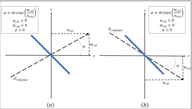
27 The angle of the relative velocity is defined as the angle between the relative velocity and horizontal axis and is computed as following:
= (2.28)
Figure 2.2 (a) shows the coordinate system and also, the relative velocity with two positive components. The angle has a positive value and is in the first quadrant. In Figure 2.2 (b) relative velocity with a negative angle is illustrated. The horizontal component is still positive but the vertical component is downward and negative. Angle is in forth quadrant and has a negative value. The sign of the angle is important to calculate the components of the forces on the ice piece in and direction.
28
2.2.2 2D force components on the ice piece
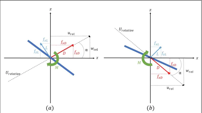
To compute the vertical and horizontal force components on the ice piece, first the lift and drag forces (aerodynamic forces) on the ice piece should be obtained. Drag force is aligned with the relative velocity and the lift force is perpendicular to the drag force. To have the force components in and directions, the sine and cosine of the will be applied to the drag and lift forces. All these force components are presented in Figure 2.3.
Figure 2.3 Aerodynamic force components on the ice piece
According to figure 2.3 (a), horizontal force ( ) and vertical force ( ) on the ice piece can be calculated as following:
29
= + (2.30)
In these equations , are the horizontal components of the drag and lift forces and , are the vertical components of the drag and lift forces.
Lift ( ) and Drag ( ) forces on an ice piece with a reference area of and the relative velocity of in a flow with a density of are:
= 0.5 (2.31)
= 0.5 (2.32)
By having the lift and drag forces, their horizontal and vertical components are:
= × , = × (2.33)
= × , = × (2.34)
Putting together all these equations gives:
= − = 0.5 ( − ) (2.35)
= + = 0.5 ( + ) (2.36)
These last two equations are used in the Matlab code to compute the force components on the ice piece and the sign and magnitude of the governs the sign of the vertical and horizontal force components. In Figure 2.3 (b) sine of the is negative and its cosine is positive so force components are: