DETERMINATION OF OPTIMAL FORGING
CONDITIONS FOR VOID ELIMINATION IN LARGE
STEEL INGOTS
by
Nathan HARRIS
MANUSCRIPT-BASED THESIS PRESENTED TO
ÉCOLE DE TECHNOLOGIE SUPÉRIEURE IN PARTIAL FULFILLMENT
OF THE REQUIREMENTS FOR
THE DEGREE OF MECHANICAL ENGINEERING
M.A.Sc
MONTREAL, SEPTEMBER, 07 2016
ÉCOLE DE TECHNOLOGIE SUPÉRIEURE
UNIVERSITÉ DU QUÉBEC
This Creative Commons licence allows readers to download this work and share it with others as long as the author is credited. The content of this work may not be modified in any way or used commercially.
BOARD OF EXAMINERS THIS THESIS HAS BEEN EVALUATED BY THE FOLLOWING BOARD OF EXAMINERS
Mr. Mohammad Jahazi, Thesis Supervisor
Department of Mechanical Engineering at École de technologie supérieure
Mr. Patrick Terriault, Chair, Board of Examiners
Department of Mechanical Engineering at École de technologie supérieure
Pierre Belanger, Member of the jury
Department of Mechanical Engineering at École de technologie supérieure
Mr. Louis-Philippe Lapierre Boire, External Evaluator Sorel Forge
THIS THESIS WAS PRENSENTED AND DEFENDED
IN THE PRESENCE OF A BOARD OF EXAMINERS AND THE PUBLIC SEPTEMBER 07, 2016
ACKNOWLEDGMENTS
The author would like to thank M.A.Sc research director, Mohammad Jahazi, for his guidance, support and expertise during the degree, without which none of this would have been possible. Gratitude is also expressed for Davood Shahriari, ETS, research assistant, for his cooperation the entire duration of the diploma.
Thanks are given to Industrial Partner, Finkl Steel, and in particular Louis Philippe Lapierre Boire, for his complete collaboration in the organisation of this project and a corresponding internship accomplished during January and February 2016. Special thanks are given again to Louis Philippe for transportation and carpooling throughout the entire internship. Appreciation is accorded for time granted off campus in this endeavour.
Gratitude is acknowledged for the Sorel Forge team, notably Rami Tremblay, Jean Benoit Morin and Stephane Roy for their help in accessing Sorel Forge information points and sample preparation. Finally, thanks are given to the forging teams especially Mario for his kind welcome and enthusiasm to assist.
DÉTERMINATION DES CONDITIONS OPTIMALES POUR L’ÉLIMINATION DES POROSITÉS LORS DE LA MISE EN FORME DES LINGOTS D’ACIER DE
GRANDE TAILLE Nathan HARRIS
RÉSUMÉ
La présence de porosités et de cavités internes est habituellement observée lors de la coulée et de la solidification des lingots de grande taille. Leur élimination et fermeture mécanique est réalisée pendant les premières déformations du procédé de transformation à chaud. Ce travail vise à déterminer les conditions optimales pour l’élimination des porosités dans des lingots de grande taille avec une attention spéciale portée au matériau et au procédé industriel utilisé. Un état de l’art présente les modèles de fermeture de porosités et les techniques de caractérisation existantes. Actuellement, il est montré que cette théorie est très peu appliquée aux lingots utilisés en industrie. Une analyse du procédé de forgeage du partenaire industriel est effectuée et différentes séquences de forgeage sont identifiées. Ensuite, une étude plus poussée utilisant des données expérimentales est proposée. Une nouvelle méthode pour le développement de modèles de fermeture de porosité est énoncée. Sur la base de cette méthode, un quotient de fonctions polynomiales est établi pour le calcul des constants matériaux. L’influence de la triaxialité et des paramètres du matériau est évaluée grâce à une cartographie 3D. Le modèle de fermeture des porosités est validé pour les aciers à hautes performances mécaniques du partenaire industriel. La fermeture des porosités est évaluée pour une séquence du forgeage libre. L’effet du positionnement des porosités est étudié. L’efficacité de la séquence de forgeage pour la fermeture des porosités est caractérisée par zone. Une combinaison originale de la fermeture relative et la vitesse de déformation volumétrique permet l’optimisation du procédé de forgeage. Un nouveau logiciel pour le forgeage libre de « slab », Forge Calculus, est développé et testé avec beaucoup de données expérimentales. Le développement à venir et notamment une prédiction de la qualité de la pièce en temps réel pendant le forgeage est discutée.
DETERMINATION OF OPTIMAL FORGING CONDITIONS FOR VOID ELIMINATION IN LARGE STEEL INGOTS
Nathan HARRIS ABSTRACT
The presence of internal voids is commonly observed throughout the casting and solidification of large size ingots. Their mechanical closure is generally achieved during the initial deformation of a hot forming process. The present work focuses on the determination of optimal forging conditions for void elimination in large steel ingots with respect to the involved materials and industrial processes. A state of the art is compiled as initial research in order to develop a solid background in void elimination theory. An extensive review of void closure models is presented and characterisation techniques are discussed. It is shown that current void closure models lack application to industrial scale forgings. An analysis of the industrial partner’s open die forging procedure ensues and characteristic forging sequences are introduced. Feasibility for further forging analysis using experimental data is evaluated and successfully proposed. A novel method for fast calculating void closure models is developed. Rational polynomial functions are established for the calculation of material dependant constants. 3D mapping is used to evaluate the influence of the triaxiality state and material parameters. The void closure model is validated for use on high strength steels from the industrial partner. Void closure is modeled and simulated during an open die forging sequence. The effect of in-billet void positioning is studied and the forging sequence effectiveness for void closure is validated and characterized for different zones. An original combination of data from relative void closure and volumetric strain rate provides a way for forging optimisation. Novel software for successful open die slab forging, Forge Calculus, is developed based on large amounts of experimental data. The in-house code provides fundamental information for setting forging standards. Future development concerning real time prediction of forging quality is discussed.
TABLE OF CONTENTS
Page
INTRODUCTION ...1
CHAPTER 1 STATE OF THE ART ...5
1.1 Introduction ...5
1.2 A modern day scale ...5
1.2.1 Macroscopics ... 6 1.2.2 Microanalytics ... 7 1.2.3 Mesoscopics ... 8 1.3 Void physics...9 1.3.1 Void origins ... 9 1.3.2 Void geometries ... 11
1.3.2.1 Simplified geometry (sphere, cylinder) ... 12
1.3.2.2 Equivalent ellipsoids ... 12
1.4 Influence of hot forging on void closure ...14
1.4.1 Principal hot forging techniques ... 14
1.4.1.1 Upsetting ... 15
1.4.1.2 Cogging ... 16
1.4.2 Influential material and process parameters ... 16
1.4.3 Material behaviour during void closure ... 17
1.4.3.1 Local thermodynamic conditions in the workpiece ... 17
1.4.3.2 Effect on the local microstructure ... 19
1.4.3.3 Healing ... 20
1.5 Comparison of existing void closure models ...21
1.5.1 STB model ... 21
1.5.2 Ragabs derived work of the Gurson-Tvergaard model ... 22
1.5.3 Budiansky’s model... 23
1.5.4 Duva and Hutchinsons modified model ... 24
1.5.5 Zhang and Cui’s analytical model ... 25
1.5.6 Zhang’s semi-analytical model ... 26
1.5.7 Saby’s CICAPORO model ... 28
1.6 Characterisation techniques ...29
1.6.1 Traditional void characterisation ... 29
1.6.2 Microtomography ... 30
1.6.2.1 3D microtomography ... 30
1.6.2.2 X-Ray microtomography ... 31
1.6.2.3 Synchrotron X-Ray microtomography ... 32
1.6.3 3D Reconstruction software ... 33
CHAPTER 2 PRELIMARY ANALYSIS OF THE OPEN DIE FORGING PROCESS ...35
2.2 Forging sequence identification ...36
2.2.1 Sequence 0: Initial forming ... 37
2.2.2 Sequence 1: Upsetting... 37
2.2.3 Sequence 2: FM process ... 38
2.2.4 Sequence 3: Cogging ... 39
2.2.5 Sequence 4: Finishing ... 40
2.3 Process variability observation ...40
2.4 Preliminary analysis ...42
2.4.1 Data collection ... 42
2.4.2 Forging sequence characterisation ... 43
2.5 Preliminary conclusions ...48
CHAPTER 3 DEVELOPMENT OF A FAST CONVERGING MATERIAL SPECIFIC VOID CLOSURE MODEL DURING INGOT FORGING ....51
3.1 Abstract ...53
3.2 Introduction ...53
3.3 Mechanical and material conditions ...56
3.3.1 Ingot breakdown process ... 56
3.3.2 Stress and material behaviour assumptions ... 57
3.4 Determination of material dependant void closure constants ...59
3.4.1 Development of material dependant model constant functions ... 62
3.5 Results and discussion ...69
3.5.1 Evolution of void closure ... 69
Void closure model comparison ... 72
3.5.2 Influence of the triaxiality state ... 74
3.5.3 Influence of material parameters ... 75
3.5.4 Characteristics of the investigated alloy ... 76
3.5.5 Material sensitivity... 77
3.6 Model validation for large size ingots based on experimental observations ...79
3.6.1 FEM simulation setup ... 79
3.6.2 In ingot sensor positioning ... 80
3.6.3 Stress and strain evaluation ... 82
3.6.4 Simulation results... 84
3.7 Conclusions ...85
3.8 Acknowledgements ...85
3.9 References ...86
CHAPTER 4 ANALYSIS OF VOID CLOSURE DURING OPEN DIE FORGING ...89
4.1 Abstract ...91
4.2 Introduction ...92
4.3 Finite element analysis ...93
4.3.1 Finite element model ... 94
4.3.2 Rheological material model ... 95
4.3.3 Void closure model ... 96
4.4 Results and discussion ...97
4.4.1 Void closure calculation method ... 97
4.4.2 FE results ... 98
4.4.3 Void closure analysis ... 99
4.5 Conclusion ...101
4.6 Acknowledgements ...101
4.7 References ...102
CHAPTER 5 DEVELOPMENT OF A PREDICTION TOOL FOR SUCCESFUL FORGING ...105
5.1 Forge Calculus – prediction tool ...105
5.1.1 In depth analysis of successful forgings ... 106
5.1.1.1 Sequence models ... 107
5.1.1.2 Sequence algorithms ... 112
5.1.1.3 Example of application ... 116
5.1.2 Individual results module ... 126
5.1.3 Statistical analysis module ... 127
5.2 Future development ...128
CONCLUSIONS...129
APPENDIX I Forging plan example ...131
APPENDIX II Main Database Structure ...133
APPENDIX III Probability function list ...135
LIST OF TABLES
Page
Table 1: Summary of presented void closure models ...21
Table 2: Values for the coefficient c1,c2 in Hutchison’s formula taken from Zhang and Cui (2009) ...24
Table 3: Values for the coefficients c1,c2,c3,c4 in Zhang's equation taken from Zhang et al. (2009) ...28
Table 4 : Indicators of process variability ...41
Table 5 : Raleigh Ritz calculated values for c1,c2 ...64
Table 6 : Raleigh Ritz calculated values for q1,q2,q3,q4 ...64
Table 7 : Relative error and statistical data verification index values ...64
Table 8 : Value of j in equation (3.8) for calculated coefficients ...65
Table 9 : Numerator coefficient values used in equation (3.9) ...66
Table 10 : Denominator coefficient values used in equation (3.9) ...66
Table 11 : 3D mapping for material dependant void closure models ...70
Table 12 : P20 chemical composition (%wt) ...77
Table 13 : Sensor positioning in billet ...82
Table 14 : Chemical composition of P20 (%wt) ...95
Table 15 : Characteristic Ingot Regions ...97
Table 16 : Void closure effectiveness per axis ...100
Table 17 : Upset results per hit of anvil ...120
Table 18 : FM results per hit of anvil ...121
Table 19 : Average Upset and FM indicators ...121
Table 20 : Cogging and Finishing average indicators ...126
LIST OF FIGURES
Page Figure 1 : Mesoscopic approach to modelling voids in large ingots taken from
(X. Zhang, 2008) ...9
Figure 2 : Void distribution in different cast Steel ingots taken from Tkadlečková et al. (2013) ...11
Figure 3 : Void geometry evolution during hot forging taken from Zhang et al. (2009) ...12
Figure 4: Definition of the dimensions and orientation of an ellipsoid taken from (M. Saby, 2013) ...13
Figure 5 : (From left to right) Transformation from real morphology to equivalent ellipsoid taken from Saby (2013) ...14
Figure 6 : Upsetting diagram ...15
Figure 7 : CV and FM models for the cogging process ...16
Figure 8 : RVE with applied boundary conditions ...18
Figure 9 : Resulting local grain orientation for various values of void to grain size ratios ...20
Figure 10 : Spherical Void Evolution for Budiansky’s HST and LST Void Closure Models...24
Figure 11 : Duva's Interpolated volumetric strain rate, Budiansky comparison ...25
Figure 12 : Void represented with a and b parameters taken from Zhang and Cui (2009). ...25
Figure 13 : Zhang semi analytical compared to other void closure models, experimental and FE results for Tx=-2 and Tx=-0.6, taken from Saby (2013). ...27
Figure 14 : X-ray tube Microtomography image acquisition principle taken from Maire et al. (2001) ...32
Figure 15 : Synchrotron X-ray Microtomography image acquisition principle taken from Maire et al. (2001) ...33
Figure 17 : 2D cross sections and consequential raw 3D image of JD20 steel
sample taken from Saby (2013) ...34
Figure 18: 63'' cast ingot after demoulding ...35
Figure 19 : The forge; 1: The press. 2: The forger's cabin. 3: The manipulator. 4: Bridge crane clamp. 5: Intermediate die. ...36
Figure 20 : Initial forming: Steps for obtaining a square base ...37
Figure 21 : Upsetting a) Left: Ingot with dish stool, b) Middle: Dish stool removal ...38
Figure 22 : FM Process...39
Figure 23 : Cogging Process...40
Figure 24 : Finishing Process ...40
Figure 25 : Typical forging position and force graph ...43
Figure 26 : Upsetting and FM characterisation ...44
Figure 27 : Cogging characterisation ...45
Figure 28 : Example of Staircase Forging ...47
Figure 29 : Finishing characterisation ...48
Figure 30 : Schematic view of concentration of shrinkage voids in a large size ingot. ...57
Figure 31 : Stress strain curve for 25CrMo4. ...59
Figure 32 : Influence of c c on volumetric strain rate. ...601, 2 Figure 33 : Influence of
{
q q q q1, , ,2 3 4}
on volumetric strain rate, Ee =0.2. ...62Figure 34 : Influence of
{
q q q q1, , ,2 3 4}
on volumetric strain rate, Ee =0.4. ...62Figure 35: The evolution of constants
{
c c1, 2}
in equation (3.1) with the Norton exponent. ...67Figure 36 : The evolution of constants
{
q q1, 3}
in equation (3.2) with squared inverse of the Norton exponent. ...67Figure 37: The evolution of constant q in equation (3.2) with cubed inverse of the 2
Norton exponent. ...68
Figure 38: The evolution of constant q in equation (3.2) with the Norton 4 exponent. ...68
Figure 39 : Void closure comparison for 14NiCrMo13, Tx = −0.33. ...73
Figure 40 : Void closure comparison for 14NiCrMo13, Tx = −1. ...73
Figure 41 : Influence of triaxiality state for 14NiCrMo13, n=7.25. ...75
Figure 42 : Influence of Norton exponent on void closure for Tx=-1. ...76
Figure 43 : Flow stress comparison between model and simplification. ...78
Figure 44 : Material sensitive void closure, Tx = −0.33. ...78
Figure 45 : Ingot geometry and meshing, mesh size 25mm. ...80
Figure 46 : Interior and exterior ingot temperature (degree C) before upsetting. ...80
Figure 47 : Internal voids (~1mm) observed from ingot cross-section. ...81
Figure 48 : Equivalent strain for large size ingot during upsetting. ...83
Figure 49 : Triaxiality state for large size ingot during upsetting. ...83
Figure 50 : Void closure for large size ingot during upsetting. ...85
Figure 51 : Ingot geometry and meshing. ...95
Figure 52 : Void positioning scheme. ...97
Figure 53 : Initial triaxiality evaluation during upsetting (t=10s). ...99
Figure 54 : Initial macroscopic equivalent strain during upsetting (t=10s)...99
Figure 55 : Accumulated equivalent deformation dependence during ingot upsetting. ...101
Figure 56 : Relative void closure during the upsetting process...101
Figure 57 : Forge Calculus main interface ...106
Figure 59 : Upsetting initial and final states ...108
Figure 60 : Cogging and finishing model ...109
Figure 61 : Billet final volume schematic ...111
Figure 62: Forging chart – First forging, 1: Upsetting, 2: FM, 3: Cogging ...117
Figure 63 : Forging chart - Second forging, Finishing ...117
Figure 64 : Upset sequence, Force filter ...118
Figure 65 : FM sequence, Force filter ...119
Figure 66 : Upset sequence, Part reduction ...119
Figure 67 : FM sequence, Part reduction ...120
Figure 68 : Cogging - Work sequence definition ...122
Figure 69 : Finishing - Work sequence definition ...122
Figure 70 : Cogging - Work sequence 19 - Travel analysis ...123
Figure 71 : Finishing - Work sequence 10 - Travel analysis ...124
Figure 72 : Cogging - Half forging completion ...124
Figure 73 : Finishing - Work sequence 10 - Part reduction with zoom ...125
Figure 74 : Individual results user interface ...127
INTRODUCTION
The size of critical metal components used in Aerospace, Transport and Energy production has evolved significantly over the last decade. Industrial needs have become slave to progress and increasingly strict client specifications. Internal defects must be eradicated before the delivery of the final workpiece in order to satisfy expectations and to stamp out all concerns of an unfaltering mechanical health during working life.
The forming process plays an essential role in the elimination of a high percentage of defects. Thus, it is at an elemental level that the future mechanical properties of the workpiece are to be decided. In the forming of ultra large ingots this entails casting and hot forging, two processes that have yet to be explicitly modelled particularly because each company possesses its own recipe. Finite model simulations are commonly used as a descriptive tool for the quantification of the physical phenomena arisen during the fabrication process. The results of which determine the framework of forthcoming process development.
The defects studied in the current work are internal voids with a particular focus on the simulation of void closure within large ingots. Void elimination typically occurs during the initial phases of the ingots elaboration notably during hot forging. It is a two part process detailing mechanical closure and a material healing mechanism. Both are necessary for successful void closure. The void volume must be reduced to zero before a final bonding of the internal surfaces may ensue.
The existing mathematical models are currently incapable of correctly predicting void closure on an industrial level. At present, the lack behind the comprehension of this phenomena makes the application of existing formula extremely case sensitive.
In association with Sorel Forge, the objective of this work is to successfully constitute a simulation prediction model for void closure. Thereby establishing criteria for the optimisation of their industrial process.
In accordance with the industrial partner, the case study focuses on large ingots with initial voids during hot forging. Void geometries and orientations vary in relation to real void morphologies. The casting process is not studied. Various grades of steel are considered. Exact proportions of the chemical composition are not divulged in order to adhere to the confidentiality clause.
This M.Sc thesis encompasses 5 chapters.
CHAPTER 1 is an extensive review of relevant literature concerning the proposed subject. This state of the art discusses the two main approaches used in void closure models. A macroscopic resolution, traditionally used for industrial purposes, and a micromechanical insight are examined before the modern mesoscopic description is addressed. The effect of hot forging on void closure and material behaviour is discussed. Different classical void closure models are compared. Microtomography, a modern characterisation technique is presented.
CHAPTER 2 is a preliminary analysis of the open die forging process. The fabrication procedure is broken down into forging sequences and potential indicators for successful forgings are selected. The feasibility of an in-depth study to characterize successful forgings based on experimental forging results is evaluated.
CHAPTER 3 features an in-depth discussion on applicable void closure models for industrial use. Existing mathematical void closure models are studied and represented using 3D mapping techniques. Significance is given to stress triaxiality states, applied remote strain and material parameters. Rational functions of the third degree are developed in order to easily adapt existing models to specific materials. Void closure is predicted for 42CrMo4, 34CrMo4 and 14NiCrMo13. A suitable model is chosen for Sorel steels.
CHAPTER 4 constitutes a FEM simulation of an open die forging sequence. Previous data and models are implemented in order to evaluate void closure. Virtual voids are introduced
for forging direction effects along a vertical, horizontal and 45 degree axis. The simulated sequence is representative of major void deformation during the hot forging process. The applied simulation method explains the efficiency of the consecutive forging sequence.
CHAPTER 5 headlines the development of a successful forging prediction simulation tool named Forge Calculus. Over 250 files of forging data are computed and analysed. The overall running of the program’s internal logic is explained and the mathematical models used for simulation prediction are detailed. Future development is discussed and highly recommended.
CHAPTER 1 STATE OF THE ART 1.1 Introduction
This chapter includes an extensive review of literature concerning void closure in hot forging, setting a solid foundation for theory development in following chapters. It contains three main concepts.
Traditional macroscopic and micro-analytical approaches to the problem of void closure are discussed before giving the advantages of the new mesoscopic approach. Details concerning the physics of void generation, growth, and closure are interpreted with importance given to the influence of hot forming in the latter stages of development. Material behaviour is analysed and local thermodynamic conditions investigated for optimal void closure. X-ray Microtomography, used to characterise void morphologies, is presented as a favourable and promising technology. Different existing mathematical models for void closure are compared. The final stage of void closure known as healing is briefly discussed, but remains annex to the current papers focus point.
1.2 A modern day scale
Many classical models of void closure use one of two perspectives to approach the problem. The chosen philosophy depends on the application and the type of results required. The scale upon which the problem is addressed affects the utility and relevance of the results obtained. A third and more modern approach to the void closure problem has been developed in recent years and serves as a proposal in this thesis’s solution.
1.2.1 Macroscopics
The macroscopic approach to the problem of void closure has become very popular and holds a great industrial interest because it focuses mainly on process parameters. Void closure mechanisms are function to process conditions, culminating in qualitative or quantitative results that are easily transposable to the working environment. Process development and optimisation are targeted in order to achieve forgings without defects. This approach generally implies experimental testing or numerical simulation.
Conclusions from Tvergaard (1982) and Ragab (2004) can be drawn that generalise the results obtained from a macroscopic process study, considering the hot forging of large ingots. The initial phases of material deformation have a strong influence on void closure. This is measured by far field equivalent strain which is seen to be a significant parameter.
Tkadlečková et al. (2013) showed the temperature gradient to affect void closure especially regarding centerline voids. A colder surface temperature improves efficiency in these areas on smaller billets (200x200mm) but seems to have no consequential effect on larger ingots given their increased thermal inertia. Heating of the workpiece to around 1250ºC prior to forging was shown to increase initial void closure rates.
Other studies by Dudra and Im (1990), indicate that the interaction between the die and billet is noteworthy. The friction coefficient was studied by Chen (2006) and the shape and angle of the contact by Kakimoto et al. (2010). The optimisation of these parameters both proved to have a positive effect on void closure in large ingots. Shaped concave anvils were shown to produce a uniform strain distribution in the early stages of hot forging significantly improving initial void closure. Asymmetric external loading and a concave geometry was proved to accentuate compressive stresses within the workpiece. Contrastively, a flat die was deemed to be advantageous in the final stages of forging as they were demonstrated to possess a greater influence on the closure of central voids by Banaszek and Stefanik (2006).
1.2.2 Microanalytics
The models used in the micro-analytical approach consist of a single void in an infinite incompressible matrix. Their formulation is based on local thermodynamic readings with less emphasis on exterior loading. Micromechanic material behaviour follows a power law derived from a stress potential in a compressible nonlinear material as showcased by Huang. and Wang. (2006). 1 0 0 0
2
3
m es
σ
ε
ε
ε
ε
−
=
(1.1)The chosen stress component, ̿ , symbolizes the deviatoric stress tensor, a fundamental element of the Cauchy stress tensor alongside the hydrostatic representation of change in volume. The distortion of volume is function to ̿ , the strain rate tensor. The other factors are: m, (0 ≤ m ≤ 1) strain rate sensitivity exponent, reference stress, and respectively reference and equivalent strain rate with
1 2
3
( : )
2
eε
=
ε ε
(1.2)Strain rate sensitivity limits represent different material make-ups from = 0, perfectly plastic to = 1, denoting a viscous nature.
Micromechanics describe local phenomenon. Their application in void closure has only been effective on simplified void morphologies. The evolution of spherical, cylindrical, Budiansky et al. (1982), and more recently ellipsoidal, Chen et al. (2014) and Saby et al. (2014), geometries have led to analytical or semi-analytical formulas. The introductory models exclude temporal shape development, therefore making them far from pertinent for modelling large deformations and consequently, industrial processes. However, the more recent models account for a change in morphology and can therefore be used in industrial process simulation.
1.2.3 Mesoscopics
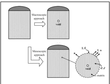
The philosophy of mesomechanics centralizes the premises of the two former approaches to void closure, achieving precise results whilst avoiding long macroscopic simulation calculation times. This perception considers the physical phenomenon at a microscopic level, governed by local thermodynamic conditions resulting from a combination of macroscopic external loadings, leading to deformations and heat transfer. Zhang et al. (2009) and Saby et al. (2013) studied void volume prediction with the mesoscale approach, both successfully creating verifiable theoretical models for the multi-scale problem using a Representative Volume Element (RVE) whilst considering the forging of large ingots. Model precision was tested against FE simulations and experimental data (Lee and Mear. 1994) with encouraging results.
Mesoscale models include substantial hypothesis in order to authentically represent the multi scale phenomenon. The vast amounts of miniature voids were assumed to have no effect on macroscopic deformation. Consequently, the initial void to billet volume ratio was deemed close to zero. Thermomechanical fields such as hydrostatic pressure or mean stress and equivalent Von Mises stress gathered from macro scale process parameters were presumed to be locally homogenous. These assumptions lead to further discussion and the implementation of certain model corrections into processing subroutines.
Mesoscopic or Mean field simulations are tools able to calculate the evolution of given parameters at any known location or integration point within the workpiece. The significant mechanical field variables concerning void closure are stress, strain and initial void morphology parameters. The Rayleigh Ritz method, a numeric solver algorithm for equations without exact answers, is used to obtain the morphology parameters for the volumetric strain rate of the proposed cell models. The criterion for material dependant void closure models depends heavily on the materials Norton and strain rate sensitivity exponent as reported by Budiansky et al. (1982), Zhang et al. (2009).
Figure 1 : Mesoscopic approach to modelling voids in large ingots taken from (X. Zhang, 2008)
1.3 Void physics
This section of the literature review aims to present a global state of the art regarding the physics surrounding voids in metal. Void growth is studied and geometries prior to deformation are analysed. It is shown that initial void morphology parameters and void shape evolution have a significant effect on the accuracy of void closure calculation.
1.3.1 Void origins
Voids initiate as a result of several process parameters, taking place during casting, leaving rudimentary defects to be trapped during solidification. Nucleation, growth and void coalescence are three microscopic phenomena that have been subject to many recent studies as in Samei et al. (2016). Traditional metallographic techniques, notably electron microscopy, as used by Song et al. (2014), have helped with the qualification of these events. Initiation is defined by the breaking down of hard particles at the interface between matrices followed by the disintegration of hard particles of the second phase, particularly inclusions.
Growth ensues, with relative kinetics, function to material parameters, stress and strain. Rice and Tracey (1969) and Budiansky et al. (1982) considered the growth of an isolated spherical
void. The former in a perfectly plastic solid submitted to a remote uniform stress and strain rate. The latter in an infinite linear and non-linear matrix material under remote axisymmetric stress due to loading conditions. Both concluded that hydrostatic tensile stress and plastic deformation stimulate void expansion.
Duva and Hutchinson (1984) worked on an incompressible power-law material lattice with spherical voids, deriving constitutive relations to predict void coalescence. Niordson (2008), expanded upon this by studying the influence of different material length parameters, defining a length scale upon which gradient hardening became important, in void growth to coalescence and identified their influence on the material’s overall mechanical characteristics. Results suggest that void growth is significantly suppressed when void dimensions are comparable to or smaller than the material’s internal length parameter. Findings that were coherent with former research by Fleck and Hutchinson (2001).
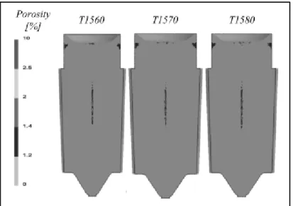
Other interpretations are that void type defects can be caused by shrinkage and gas progression during solidification. Tkadlečková et al. (2013) and Saby (2013) collected data as to the location of porosities in extra-large cast ingots. Results showed higher void densities along ingot centerlines and in the upper regions (Fig 2.). The formation of voids at statistically backed locations could also be due to the surrounding microstructure. Carroll et al. (2012) studied the effect of grain size on local deformation near void-like structures, concluding that the size of strain concentration features are comparable to the materials local grain size as will be further developed in 1.5.2.
Figure 2 : Void distribution in different cast Steel ingots taken from Tkadlečková et al. (2013)
1.3.2 Void geometries
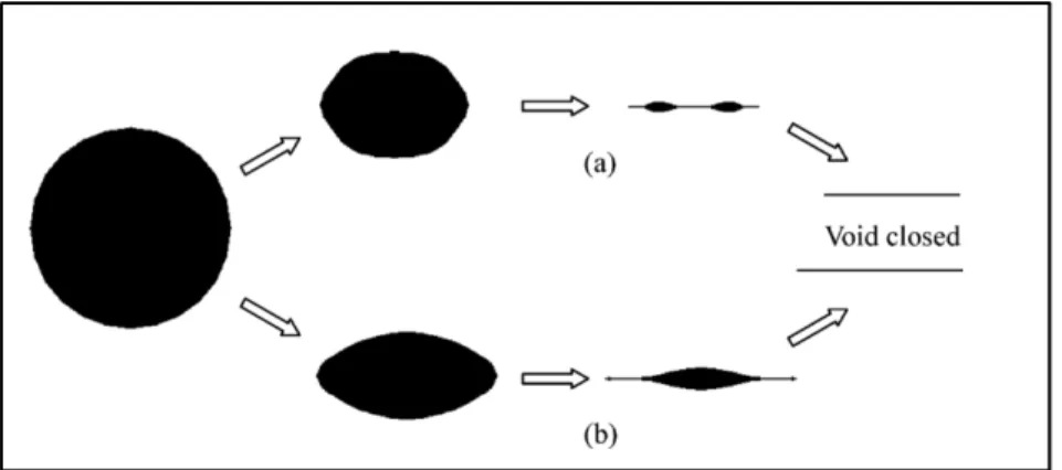
It is industrially inconceivable that all void morphologies be modelled with complex real geometries. Despite the apparition of numerous analytical, semi-analytical and numeric models, none allow for real geometry perception. Modern modelling considers spherical, cylindrical and equivalent ellipsoidal voids. Works on void closure by Rice and Tracey (1969) and Budiansky et al. (1982), propose the conservation of a spherical void during hot forging. Later papers including Zhang et al. (2009) and Saby (2013) envisage an evolution of the voids morphology over time. These considerations lead to more accurate results concerning current closure states. Real mean-field simulations show 3D void shape metamorphosis on a 2D plane from sphere to ellipsoid to crack (Figure 3). It must be noted that this evolution path shows an excellent analogy with real void closure results by Lee and Mear (1999).
Figure 3 : Void geometry evolution during hot forging taken from Zhang et al. (2009)
1.3.2.1 Simplified geometry (sphere, cylinder)
Traditional void closure models, Budiansky et al. (1982), Rice and Tracey (1969) or newer works from Chen et al. (2014) use simplified geometry in order obtain workable, analytical functions. Geometries include isolated spherical voids, circular-cylindrical and elliptic cylindrical voids. The latter will be discussed in a following paragraph.
Spherical models show good correlation to real void closure during initial stages of deformation. Significant error can occur for higher values of effective strain. This is explained by the fact that the current models do not consider void shape transformation. The initial spherical void remains spherical until completely closed.
Initial void morphology parameters are also considered significant. Accurate simulations depend on the adaptability of the model to compensate for the evolution of void geometry during the forging process.
1.3.2.2 Equivalent ellipsoids
More recent works from Saby (2013) and Zhang et al. (2012) introducing respectively the Zhang and Cisco models, use initial void geometry parameters; {qi∈[0, 4]}. The error of
these two models compared to real geometries is shown to be of 5% for the majority of voids encountered. The method details equivalent ellipsoids, calculated via inertia matrices to represent actual voids.
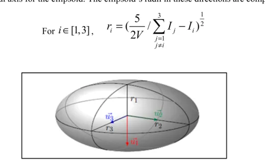
Inertia matrices can be calculated and implemented into source code as a subroutine at each integration step. The internal surfaces of a void were considered. Three node triangular elements were used and a homogenous unitary density supposed. The position of each of the three vertices , , of each finite element were used to obtain access to the diagonal components of the voids inertia matrix.
For
i
∈
[1,3]
, 3 1 i ij j j iMI
P
= ≠=
(1.3) With Pij = f vol T(( )
r , , , , )O A B C (1.4) being the triangular element of integration. The three strictly positive principal inertia moments , , are considered in order to calculate equivalent void dimensions , , . The eigenvectors, defined in an orthonormal basis , , , represent the three principal axis for the ellipsoid. The ellipsoid’s radii in these directions are computed as:For
i
∈
[1,3]
, 1 1 3 25
(
/
2
)
i j i j j ir
I
I
V
= ≠=
−
(1.5)Figure 4: Definition of the dimensions and orientation of an ellipsoid taken from (M. Saby, 2013)
FE simulations were prepared using the equivalent ellipsoid approximation after real void morphologies were identified using x-ray tube microtomography. Numerical inconsistences were exposed in the latter stages of void closure corresponding to the contact between internal surfaces. Nevertheless, even for tortuous voids, this transpired after 80% of void closure had already occurred.
Figure 5 : (From left to right) Transformation from real morphology to equivalent ellipsoid taken from Saby (2013)
1.4 Influence of hot forging on void closure
Forging processes are an essential step in the fabrication of a sound material. Void closure requires energy, in the case of hot forging, an increase in temperature coupled with energy transferred from exterior loadings in the form of plastic deformation, strain energy and void surface energy is produced. A major secondary effect is the activation of particle diffusion, necessary in the healing stages of void closure.
1.4.1 Principal hot forging techniques
A handful of hot forging techniques are used in today’s industrial climate. Open die forging or smith forging is paramount for workpiece sizes debuting as large ingots. Closed die forging is used for smaller parts and will therefore be omitted. The process of Upsetting and Cogging make up the prominent duo that lay the foundation a forging fabrication process. A brief description of these two hot forging operations follows.
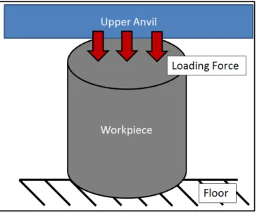
1.4.1.1 Upsetting
Upsetting is a shape transformation technique for cast ingots in hot forging that consists in applying pressure to one side of a workpiece along its principal axis with flat a die. The aim of this process is a reduction in height which comes accompanied by an increase in width of the workpiece. Main process parameters include initial and final die heights. Heat transfer conditions and existing friction between die face and ingot can cause barreling if left unmonitored. Azushima et al. (2012) showed that the correct choice of lubricant can significantly reduce this phenomenon. High viscosity lubricants allowing for uniform displacements. Low viscosity fluids were shown to create a non-uniform distribution, increasing from the counterpoint to the periphery.
The compressive forces fathered from the upsetting process can be beneficial to the closure of internal voids or other defects engendered during casting. Lee et al. (2011) determined a non-unique response in void closure to upsetting. Various void behaviours were observed, depending on size and position in the large ingot. Hydrostatic stresses around the void were shown to switch from tensile to compressive to tensile conditions. Effective strain of over 0.6 was indicated to validate void closure conditions.
1.4.1.2 Cogging
Cogging or drawing out often follows the upsetting process in the forging of long, square, octagonal or circular sectioned, steel slabs. The operation takes place in steps, generally starting at one end of the workpiece and finishing at the other. The repetition of these steps is alternated with the rotation of the workpiece in order to reduce thickness and increase length.
Cho et al. (1998) investigated the cogging process design using Conventional flat (CV) and Free Mannesmann (FM) dies (Figure 7). FM dies proved more efficient, increasing hydrostatic stresses in the ingots center. Bite width was also evaluated, concluding that optimal parameters were obtained using 40 to 75% of the width of the die. Quicker forging can be accomplished using a smaller bite, increasing thickness reduction. Kakimoto et al. (2010) demonstrated that a reduction ratio of 75% was necessary in order to achieve soundness in the material matrix.
Figure 7 : CV and FM models for the cogging process
1.4.2 Influential material and process parameters
The deformation occurred by applied external loading during industrial processes have been found to be the main source of void closure. Hydrostatic pressure was shown to be of high importance by Keife and Ståhlberg (1980) and the parameter, Q, based on this characteristic
was established by (Tanaka et al. 1986). The variable is calculated as the integral of stress triaxiality with regards to equivalent deformation.
0
x
Q
= −
ε
T d
ε
(1.6)A void closure parameter (VCP) was later proposed using numeric integration. Further work by Kakimoto et al. (2010) emitted a threshold value Q ≥ 0.21 for complete closure of an axisymmetric cylindrical drilled hole. The method for process optimization gave encouraging results. However, the modelling of an internal void with only drilled through hole could be seen as unrealistic and too simplistic, giving way for debate. More recent work by Chen and Lin (2013), extended the void closure criterion to a tridimensional space, using a phenomenological expression to correlate the established functions to ellipsoidal voids. FE simulations were used to identify model constants relative to void locations within the workpiece.
Works by Gurson (1977), Budiansky et al. (1982), Duva and Hutchinson (1984),Ragab (2004), Zhang and Cui (2009) and Saby (2013) all emphasise the importance of a trio of process and material parameters. The first, relating to the Q parameter is the stress triaxiality ratio. The second, hand in hand with the hot forging process is the level of deformation, directly related to the industrial process. The final parameters are the materials Norton and strain sensitivity exponents. The analysed void closure models that appear later in this work hypothesise a direct relationship between these two entities.
1
n
m
=
(1.7)1.4.3 Material behaviour during void closure
1.4.3.1 Local thermodynamic conditions in the workpiece
Process loading paths are directly responsible for internal void closure during hot forging. The application of a significant pressure and temperature induces a modification to
mechanical parameters such as strain, strain rate and internal stress on an elemental level. The modelling of this process typically includes a Representative Volume Element (RVE), or a cube of material, presented in Figure 8. Classic local thermodynamic boundary conditions are defined such as mesoscopic loading conditions given by Saby et al. (2013). The considered RVE possesses conditions of symmetry on three adjoining faces. Normal pressures σ σxx, yy and a given velocity V are applied to the remaining faces. RVE z
dimensions are subject notably to the dimensionless volumetric ratio,
η
, respectively void over cube. This ensures parameter homogeneity in the cube, a necessary initial hypothesis.Works including Saby (2013) and Tkadlečková et al. (2013) show the majority of voids and cavities to be located along the centerline and upper half of extra-large ingots. Boundary conditions for the represented RVEs are to be found using full field simulations. Adopting the mesoscale approach means defining selected positions within the ingot used as a basis for future analysis to provide the necessary thermodynamic RVE loading information. Importance is given to ensuring homogenous mechanical variable values for each calculated time step. Current mathematical void closure models, lacking the effects of local microstructure, validate the former premise.
Figure 8 : RVE with applied boundary conditions Taken from Saby (2013)
1.4.3.2 Effect on the local microstructure
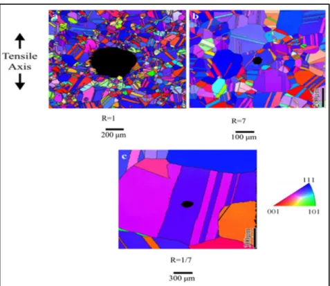
Very little research has appeared on the effect of the local microstructure on void aspects in crystalline materials. Carroll et al. (2012), however, analysed the effect of local grain size on stress concentration around a void-like structure. A Dimensionless parameter denoting relative void to grain size was adopted in order to quantify the phenomenon. Grain size and anisotropy were shown to have a significant influence over the dominant mechanism causing strain in the material around the void. For a void to grain size ratio of 1 or less, the stress of a cylindrical through hole was commanded by the grain anisotropy whereas the effect was lesser for larger ratios. Concluding remarks on material behaviour were that the closer the characteristic void dimensions came to the microscopic scale (grain size), the more local elastic and plastic deformation were affected by the fluctuation in grain heterogeneity and grain orientation, see Figure 9. This was demonstrated with data collected using the Scanning Electron Microscope (SEM) and Electron Backscattered Diffraction (EBSD) measurements.
Even if the work was solely linked to grain size, it gives thought to how the microstructure may affect void closure during hot forging. If anything, it has proven the necessity to adjust classical void closure models and FE simulations to account for microstructural conditions. Roux et al. (2013) noticed this tendency and created a level set and anisotropic adaptive remeshing strategy for the modeling of void growth under larger plastic strain.
Figure 9 : Resulting local grain orientation for various values of void to grain size ratios
1.4.3.3 Healing
Park and Yang (1996) deduced the existence of two stages in the closing of voids in large ingots, healing qualifying as the second stage in successful void closure. The current work isn’t focused on this aspect of the closure mechanism. Nevertheless, it was found to be beneficial in understanding future challenges.
After mechanical closure, the void’s volume has been theoretically reduced to zero. Contact has been achieved between internal surfaces and bonding must begin in order to restore superior material mechanical properties. The completion of this phase indicates a sound workpiece. Song et al. (2014) emitted the following basic assumptions and key issues with healing. Primary factors include the provision of material and energy. Fundamental sources incorporate internal surfaces, the material lattice and interface diffusion. Energy is provided
through exterior loading and temperature gradients. Diffusion plays an overriding role during the process and therefore implies a strong dependency on the materials chemical make-up. Several notable stages were defined. An initial fast healing stage followed by a reduction in healing speed. Closing stages displayed acceleration in healing caused by surface and interface diffusion. The completion of the healing process was shown to be controlled by lattice diffusion.
1.5 Comparison of existing void closure models
This section gives up to date compilation and comparison of existing void closure models, each using its own set of hypothesis, justified by the studied working scale. This extensive analysis considers models potentially viable for application to industry. Table 1 summarizes the reviewed void closure models.
Table 1: Summary of presented void closure models
1.5.1 STB model
The Stress Triaxiality Based (STB) Model was first used in Forge ®, a finite element forge prediction software, as a user defined subroutine implemented by Lasne (2008). The
Model Scale Type Constants Equation Tendency
STB Macro Empirical Kc=5 Eq. (1.8) Linear Ragab (2004) derived from
Gurson-Tvergaard
Macro Analytical q1=1.5,q2=1 Eq. (1.10) Exponential
Budiansky et al. (1982) Micro Analytical Eq. (1.11) Exponential
Duva and Hutchinson (1984) Micro Analytical c1,c2, (Table 2) Eq. (1.13) Exponential
Zhang and Cui (2009) Meso Analytical Eq. (1.17) Exponential
Zhang et al. (2009) Meso
Semi-Analytical
c1,c2,c3,c4 (Table 3) Eq. (1.18) Exponential
description is a simplest function correlating void volume variation with stress triaxiality ratio and incremental strain. Considering a constant stress triaxiality ratio and the absence of any initial strain, an affine void closure function can be deduced, as shown in Equation (1.8).
0
1
c xV
K T
V
= +
ε
(1.8)The value of Kc ≈ was obtained through a series of simulation tests looking at spherical 5 voids in a cuboid matrix. The numerical constant is also preprogrammed into Forge2011. The function’s slope becomes negative taking into account a compressive material state (Tx < ), 0 and the strain range limited to 0, 1
c x
K T ε ∈ −
. The model’s limitations, induced by a
macroscopic approximation, explain the discrepancies observed with real void closure. The model was observed to converge rapidly, overestimating the effect of far field strain on void closure for higher strain values.
1.5.2 Ragabs derived work of the Gurson-Tvergaard model
Introduced in 1977, Gurson (1977) established a model for rigid perfectly plastic porous materials. This considered state is denoted mathematically as m→0, Equation (1.7). Void evolution is based on the void volume fraction, f , present in the workpiece, and the plastic strain rate tensor, εpl.
(1 ) ( pl)
f = − f tr ε (1.9)
Solely focusing on void closure, Ragab (2004) simplified Gurson’s yield function hypothesising axial symmetric void deformation in order to formulate an expression to evaluate the volumetric strain rate
e
V E V
. In the case of compressive stresses, Tx ≤ , the 0
integrated void closure function can be expressed as 1 2 2 0
3
3
exp
sinh
2
2
e xq q
V
E
q T
V
=
−
−
(1.10)The values of the numerical constants were determined by Tvergaard (1982) upon Gurson’s yield criterion. The calculated values are q1 =1.5andq2 = , corresponding to the closure of a 1 continuously spherical void. Other authors have alleviated the initial expression of void volume fraction, but these studies do not correlate with the framework of the current thesis. Although widely used in void closure prediction models, the mathematical expression fails to account for material dependency.
1.5.3 Budiansky’s model
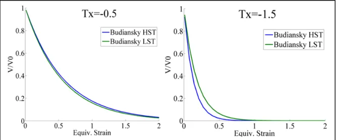
Budiansky et al. (1982) and derived works from Tvergaard (1984) provided mathematical models for nonlinear viscous materials. Two formulae were obtained using the Rayleigh-Ritz Method as analytical solutions were shown to be infeasible. The respective equations were assigned to high and low stress triaxiality (HST, LST) rates. Low stress triaxiality being defined for T x 1. Both formulae show similar results for stress triaxiality rates close to 1.
Discrepancies between the two models are observed for Tx≠1, see Figure 10. Under compressive stress the HST volumetric strain rate is integrated as follows.
1 0 3 3 exp ( ) 2 2 HST m e x sph V m E T G m V = − − + (1.11) With ( ) (1 )(1 2 ) 9 3 G m = −m + π , ∀ ≤ Tx 0 (1.12)
Figure 10 : Spherical Void Evolution for Budiansky’s HST and LST Void Closure Models
1.5.4 Duva and Hutchinsons modified model
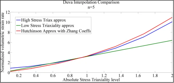
Duva and Hutchinson (1984) added the c1 and c2 coefficients to Budiansky’s model, creating a unique volumetric strain function (1.13) for both Low and High Stress Triaxialities. The model successfully corrects the underestimation of the effect of the deformation rate in Budiansky’s HST model as a consequence of its velocity field hypothesis. A comparison between all three models is available in Figure 11.
1 1 2 0 3 3 exp ( ) 2 2 m e x x sph V E mT G m c T c V = − − + − + (1.13)
The factors c1, c2 are strain rate sensitivity-dependant. The corresponding values were indexed by Zhang and Cui (2009) using the Rayleigh Ritz method and can be found in Table 2.
m 0.01 0.1 0.2 0.3 0.5 1.0
c1 1.0066 0.9002 0.7061 0.8049 0.5951 0
c2 -0.8329 -0.7874 -0.6571 -0.7340 -0.5479 0
Table 2: Values for the coefficient c1,c2 in Hutchison’s formula taken from Zhang and Cui (2009)
Figure 11 : Duva's Interpolated volumetric strain rate, Budiansky comparison
The interpolated function admits a maximum error of around 25 percent for extreme Norton exponent values and for stress triaxiality states close to 1 in comparison to both Budiansky’s HST and LST approximations and their respective intervals of validity.
1.5.5 Zhang and Cui’s analytical model
Zhang and Cui (2009) proposed a void closure model capable of predicting void closure accounting for void shape evolution during hot forging in regards to its shape parameter
a b
λ = , representing the quotient of the voids semi minor and major axes, see Figure 12. Special values of this coefficient are obtained for
λ
=1 and forλ
→0, depicting respectively a spherical void and a penny shaped crack.Figure 12 : Void represented with a and b parameters taken from Zhang and Cui (2009).
The volumetric strain rate for a sphere is given by Duva and Hutchinson (1984) , application of Equation (1.14) for any value of stress triaxiality.
1 1 2 3 3 ( ) 2 2 m sph x x m D = T +G m +c T +c , ∀ Tx (1.14)
The Rayleigh Ritz procedure and the variational principle were also applied to the amended analytic function by He and Hutchinson (1981) and the following approximate volumetric strain rate was identified.
1 6 2 3 1 3 cr x D T m λ λ π = + + for
λ
1 (1.15)In order to correlate with Budiansky’s formula (1.11) for spherical voids with m=1 a closed form expression is calculated. Here λ is the change rate of the void’s aspect ratio.
3 3 2 2.5 (1 ) (29 45 ) 1 3 2 9 e x D m m E T λ
λ
= = − − − + − − (1.16)The conclusion of Zhang’s aspect crack ratio work was a model that accounted for the transition from a spherical void to a penny shaped void during the latter stages of closure. The change in void volume relatively to the matrix is shown to be dependent on the materials Norton exponent, stress triaxiality and effective strain as far field variables.
0 exp( ) exp( ) exp( ) cr e cr e sph e cr D D E D D E V D E V D D λ λ λ − − − = − (1.17)
The formula is a weighted relative error between the crack like form and the change rate aspect balanced by the volumetric strain rate for spherical voids.
1.5.6 Zhang’s semi-analytical model
Further work, Zhang et al. (2009) , established a criterion focusing on the macroscopic strain effect during void closure. An initially spherical void was considered and void shape change accounted for. Four constants were introduced and calculated using FE simulations on a cubic cell model under axisymmetric remote stresses, see Table 3. The formula for void
volume evolution, Equation (1.18), was obtained after integration of the volumetric strain rate. 1 2 4 1 2 3 4 0 3 3 exp ( ) 2 2 m e x x e e V m E T G m c T c E c E c V = − + + + + + (1.18)
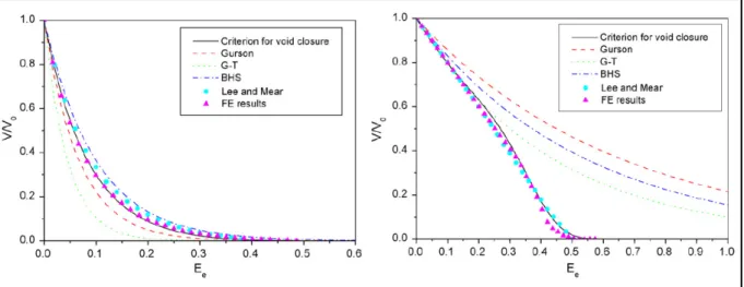
Numerical simulations with this model were shown to be in good correlation with data obtained by Lee and Mear (1999). This model shows greater accuracy when compared with classical damage definitions in the case of void closure. Significant evolution of an initial spherical void occurs, collapsing in latter stages due to internal surface contact, explaining the decrease in the collapse rate. FE simulations were also developed and compared to the former description. Again, the results showed a stronger correlation to the semi-analytical void closure model in comparison with other classical models, particularly for lower stress triaxiality states.
Figure 13 : Zhang semi analytical compared to other void closure models, experimental and FE results for Tx=-2 and Tx=-0.6, taken from Saby (2013).
m 0.01 0.1 0.2 0.3 0.5 1.0
c1 6.5456 2.9132 0.6016 1.1481 0.4911 0.5048
c3 324.4417 185.5622 72.6397 108.2114 53.8018 14.2610
c4 -1.9575 -0.6511 -0.1243 -0.2480 -0.2314 -0.3379
Table 3: Values for the coefficients c1,c2,c3,c4 in Zhang's equation taken from Zhang et al. (2009)
1.5.7 Saby’s CICAPORO model
Introduced in 2013, the CICAPORO model represents void closure with a strong emphasis on initial void geometry. Morphology equivalent ellipsoids are used and the matrix material follows the Hansel-Spittel law:
4/( 0) 0
(
0)
m n mA
e
ε εσ
=
ε ε ε
+
+ (1.19)This description denotes a dependency both on strain hardening and softening, n m and on , 4 strain rate sensitivity, m . The value of A characterizes a model optimisation parameter. The current material behavior law is an extension of Budiansky et al. (1982) and Tvergaard (1984) for a strain rate sensitivity depend-only model. An analytical function was chosen as
2 0 V A B C V = +
ε
+ε
(1.20)The initial void volume condition implies that A be equal to 1. The numerical value of the B and C criterion depends on case sensitive parameters.
3 2 1 1 0 0
( ) ( )
k j jk x i i i j kB
b T
γ
p
= = ==
(1.21) 3 2 1 1 0 0( ) ( )
k j jk x i i i j kC
c T
γ
p
= = ==
(1.22)Thep symbolize linear dependant void orientation, i T the stress triaxiality ratio, and x γia non-dimensional geometric ratio between initial void volume and ellipsoid principal direction radii. The bjk and cjkcoefficients were obtained using different regression techniques.
Void closure in advanced stages,
0
0.2
V
V ≤ , was shown to be less accurate because of the chosen ellipsoid shape evolution. However comparison with real void morphologies for closure ∈
[
1, 0.2]
displayed an excellent likeliness.1.6 Characterisation techniques
This section describes the main modern-day non-destructive void characterisation techniques used in metal forming industries. The main challenge lies in the size of the final workpiece. Void detection in large ingots is possible. However, current high resolution void analysing and visualisation technology is only available for smaller metal samples. The acquisition of a tri-dimensional image is not only used to characterize the void’s morphology, but also implemented in FE software, meshed and simulated to study a materials susceptibility to void closure.
1.6.1 Traditional void characterisation
Upon realisation of insufficient mechanical health due to void apparition, industries would traditionally use destructive metallographic techniques to analyse the extent of development. For obvious reasons, non-destructive characterisation techniques were deemed preferential leading to the adoption of ultrasonic waves for the metal working environment. Defect detection via ultrasound for on the spot structural health monitoring persists today as a viable inspection technique as shown by Zhang (2016).
The physical principle is simple. The variations of wave echoes are interpreted as a modification in the studied materials internal structure. The emitted regular wave pulse is disturbed by the presence of discontinuities such as voids or inclusions and reflected back to the detector. The received electronic signal is analysed and visualised on screen as intensity vs distance. High intensity pics symbolise flaw detection. Ultrasonic testing provides the advantage of being able to investigate internal material structure not only on the surface but
also in the bulk of the workpiece. Difficulties in the application of this technique include surface curvature, roughness and lack of parallelism.
Szelążek et al. (2009) studied the application of acoustic birefringence as a measurement for the evaluation of material degradation. An encouraging technique for void detection in metal samples was found to depend on shear wave velocity changes. A shear wave is propagated in the direction of material thickness and polarized in two orthogonal directions, those of the materials acoustic axis. The birefringence, B, in steels, depends on material texture or preferred grain orientation and internal material stress state. The measure of acoustic anisotropy is calculated as in Equation (1.23):
12 13 13 12 12 13 13 12 2.V V 2. t t B V V t t − − = = + + (1.23)
V12, V13 the velocities of the shear wave and t12, t13 their respective time of flight in the direction 1, polarized along 2 or 3. It is interesting to note that this expression of birefringence is independent of actual material thickness at the time of measure. Wave velocities were found to be function of void densities, size and orientation in comparison with the wave’s direction of propagation, therefore proving this technique to be a significant quantification parameter for the detection of internal defects.
1.6.2 Microtomography
1.6.2.1 3D microtomography
3D Tomography is an imaging technique through sectioning. The basic principal lies with the materials interaction to a penetrating wave. The information received by the equipment’s detectors is reconstructed to form 2D cross sections of the analysed sample. The 2D sections are cross referenced with a projection of the 3D form and reconstruction algorithms are used to generate a 3D image. The advantages of this technology lie in the precision of the reconstructed image and the range of material application including metal matrix composites, metallic foams and alloys. The current method of identification is often employed for
studying microstructures or material defects such as inclusions, pores and voids as studied by Lecarme et al. (2014). The clear visualisation of the internal structure incorporates an improved shape description and has led to a breakthrough in applied 3D material modelling. This technique also caters for real time experiments including material compression. Observations encompass images differentiating between the workpiece’s core and surface.
1.6.2.2 X-Ray microtomography
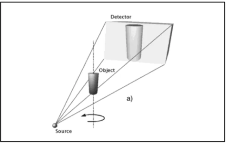
X-ray microtomography is a recent widely-used non-destructive tridimensional material analysis technique. Scientific application was studied by Maire et al. (2001). As in any tomography technique the acquisition of a 3D image requires two stages. The first entails obtaining sampled information, the second details its reconstruction. The sample is placed on a rotating support between the detector and the x-ray source. In general one complete rotation will become hundreds of images. The precision of the tomograph is function to the preprogrammed angular discretization. Initial x-ray technology used an x-ray tube as the source of photon emissions. The resulting image resolution reached 10 microns voxel size. Photons are accelerated by means of a difference in electric potentials ranging from 220kV and 450kV. Each sample must be studied to find optimal imaging parameters. Image sharpness is function to the sources focal. A radiograph obtained using a reduced acceleration tension will emit a sharper image, but can only be used on a sample with reduced thickness. To the contrary, larger samples require more energetic photons, reducing radiograph quality. The consequential beam emitted by this technology has the form of a cone, see Figure 14. (Lee et al. 2007) studied a porous steel specimen displacing the object in the x-ray tube’s conic beam thus achieving magnification of the final image.
Figure 14 : X-ray tube Microtomography image acquisition principle taken from Maire et al. (2001)
Beer-Lamberts law is used to associate the materials attenuation coefficient, alpha, to the beam’s intensity.
( D) 0
I
=
I e
−α (1.24)0
I is the incident intensity and D the length of the path travelled by a photon.
1.6.2.3 Synchrotron X-Ray microtomography
The most recent micro-tomographs use synchrotron lighting. The last decade has proved this new technology to be more clear-cut than its predecessors. Frequently used for steel imaging, the light source provides a more energetic wave resulting in a higher percentage of material interaction, consequently improving image precision. Used to study the evolution of voids under compression in steel and other alloying metal samples, Everett et al. (2001) and Toda et al. (2009) obtained tri-dimensional images providing a resolution around 1μm voxel size. Unlike x-ray tube technology a parallel beam is emitted by the source, see Figure 15.
Figure 15 : Synchrotron X-ray Microtomography image acquisition principle taken from Maire et al. (2001)
1.6.3 3D Reconstruction software
Various reconstruction algorithm software exist that produce a 3D grayscale image after numeric treatment of the 2D projections. The resulting imaging depends notably on the 2D radiographs taken during the 360o snapshot session. The detectors sensitivity range and transmitted light intensity are key factors to the amount of noise present on the final render. Image filtering is applied to eliminate unwanted noise. The median filter was shown to produce encouraging results, omitting greyscale noise without compromising image sharpness. The presence of lighter and darker zones is the result of a beam interaction surface phenomenon such as beam hardening and reflection. Treatment of these image defects include the background subtraction or Rolling Ball algorithm, established by Sternberg (1983). A decision is made on the level of details to be eliminated after computation of a background image, excluding extreme light and dark zones. Saby (2013) used x-ray tube micro-tomography to determine the presence of voids in a JD20 sample, see Figure 16.
Figure 16 : 2D cross sections and consequential raw 3D image of JD20 steel sample taken from Saby (2013)
CHAPTER 2
PRELIMARY ANALYSIS OF THE OPEN DIE FORGING PROCESS 2.1 Industrial partner and process selection
The current M.A.Sc was carried out in collaboration with FINKL Steel, a metal transformation company specialised in high performance steels. Time was accorded to visit one of the subsidiaries, Sorel Forge, in order to analyse the current open die forging process.
Sorel Forge manufactures numerous parts, all various sizes. The largest cast ingot is 63 inches in diameter and was selected for initial geometry in order to respect the framework of this thesis.
The shape most often forged from the 63’’ ingot is a parallelepiped, and more precisely, a rectangular prism. Internally, the process is known as slab forging. This process was selected for the current study.