Dam-break flow computation using high resolution DEM

Fourth International Conference on Advanced COmputational Methods in ENgineering (ACOMEN 2008) Editors: M. Hogge, R. Van Keer, L. Noels, L. Stainier, J.-P. Ponthot, J.-F. Remacle, E. Dick ©University of Liège, Belgium, 26-28 May 2008

Dam-break flow computation using high resolution DEM

S. Erpicum

1*

, B.J. Dewals

1,2

, P. Archambeau

1

and M. Pirotton

1

1

HACH Research Unit, ArGEnCo Department, University of Liège Chemin des Chevreuils, 1 B52/3, B-4000 Liège, Belgium

2

Belgian National Fund for Scientific Research F.R.S-FNRS

e-mails: {S.Erpicum, B.Dewals, Pierre.Archambeau, Michel.Pirotton}@ulg.ac.be

Abstract

Dam-break flow computation is a task of prime interest in the scope of risk analysis processes related to dams and reservoirs. High resolution Digital Elevation Models (DEMs) available today provide extremely dense and accurate topography information in the valley downstream of these structures, even in urban area. In this paper, a 2D finite volume flow solver, able to deal with these DEMs, is presented in details. Validation examples are comprehensively described.

1 Introduction

Dams and reservoirs are recognized for their valuable contribution to the prosperity and wealth of societies across the world, while they are also blamed for their risk of failure. Failures of large dams remain fortunately very seldom events. Nevertheless, a number of occurrences have been recorded in the world, corresponding in average to one to two failures worldwide every year. Some of those accidents have caused catastrophic consequences, but past experience reveals also that loss of life and damage can be drastically reduced if Emergency Action Planning (EAP) is implemented in the downstream valley. The development of EAP is an outcome of a complete risk analysis process, which requires, among other components, a detailed prediction of the propagation of the flood wave induced by the dam failure.

In this general scope, since practical risk analysis must be applicable for long real valleys at a sufficiently high space resolution, depth-averaged hydrodynamic models still constitute the most appealing approach. Nevertheless, numerical modelling of such flows involves numerous challenges to be taken up. First, the flow is characterized by a highly transient behaviour involving the propagation of stiff fronts. Therefore, a proper upwind numerical scheme is required for the computation to be stable, while a satisfactory accuracy must be reached in space and time. Secondly, conservation of physical quantities must be preserved during wetting and drying of computation cells. Finally, the hydrodynamic model must be able to deal with flows over natural topographies, which are inherently irregular. The conservation of momentum and energy requires a suited discretization of the source term representing the bottom slope.

At the University of Liege, a pioneering work was conducted by Pirotton [1] in the early nineties, leading to 1D simulations of dam break flows on natural topography and to their validation by physical modelling. Based on an upwind finite element scheme, the simulation time exceeded one week to run on 200 cells. Today, a corresponding 2D model is run in less than one day on a 200,000-cell grid. Based on a finite volume scheme, this 2D hydrodynamic model, called WOLF 2D, handles multiblock regular grids and includes turbulence modelling as well as a specific iterative process to simulate wetting and drying of computation cells without mass or momentum error.

Following extensive validation by comparison with theoretical, experimental and field data, the 2D model has proved its efficiency and reliability. In addition, the availability of high resolution Digital Elevation Models, directly usable with the flow solver, makes possible huge improvements in the numerical modelling of the flow field propagation in urban areas for example. As a consequence, the combination of both an efficient and up to date numerical model and high resolution DEM, presented in this paper, enables dam break flow computations in a very accurate, finely distributed and reliable way. This approach provides thus entry data of prime interest for EAP setting. It has subsequently been applied

for practical risk analysis in Belgium and abroad. This model and some validation test cases are presented in details in the following paragraphs.

2 Hydraulic model description

2.1 Mathematical

model

The 2D hydraulic model is based on the two-dimensional depth-averaged equations of volume and momentum conservation, namely the shallow-water equations (SWE). In the “shallow-water” approach, the only assumption states that velocities normal to a main flow direction are significantly smaller than those in this main flow direction. As a consequence, the pressure field is found to be almost hydrostatic everywhere. The large majority of flows occurring in natural valleys, even highly transient, can be reasonably seen as shallow, except in the vicinity of some singularities (e.g. weirs). Indeed, vertical velocity components remain generally low compared to velocity components in the horizontal plane and, consequently, flows may be considered as mainly two-dimensional. Thus, the approach presented in this paper is suitable for many of the problems encountered in river management as well as for dam break modelling.

The conservative form of the depth-averaged equations of volume and momentum conservation can be written as follows, using vector notations:

0 d d t x y x y ∂ ∂ ∂ ∂ ∂ f + + + + = − ∂ ∂ ∂ ∂ ∂ f g s f g S S (1)

where is the vector of the conservative unknowns. f and g represent the advective and pressure fluxes in directions x and y, while f

[

T

h hu hv

=

s

]

d and gd are the diffusive fluxes:

2 1 2 hu hu gh huv ⎛ ⎞ ⎜ ⎟ =_⎜ + _⎟ ⎜ ⎟ ⎝ ⎠ f 2 _, 2 1 2 2 hv huv hv gh ⎛ ⎞ ⎜ ⎟ = ⎜ ⎟ ⎜ ₊ ⎟ ⎝ ⎠ g , d 0 x xy h σ ρ τ ⎛ ⎞ ⎜ ⎟ = − ⎜ ⎟ ⎜ ⎟ ⎝ ⎠ f , d 0 xy y h τ ρ σ ⎛ ⎞ ⎜ ⎟ = − ⎜ ⎟ ⎜ ⎟ ⎝ ⎠ g . (2)

S0 and Sf designates respectively the bottom slope and the friction terms:

[

]

T

0 = −gh 0 ∂zb ∂x ∂zb ∂y

S Sf =⎡⎣0 τbx∆Σ ρ τby∆Σ ρ⎤⎦T (3)

In equations 1 to 3, t represents the time, x and y the space coordinates, h the water depth, u and v the depth-averaged velocity components, zb the bottom elevation, g the gravity acceleration, ρ the density of

water, τbx and τby the bottom shear stresses, σx and σy the turbulent normal stresses and τxy the turbulent

shear stresses. Consistently with Hervouet [2],

(

) (

2

)

2

b b

1 z x z y

∆Σ = + ∂ ∂ + ∂ ∂ (4)

reproduces the increased friction area on an irregular (natural) topography [3].

2.2 Friction

modelling

The bottom friction is conventionally modelled thanks to an empirical law, such as the Manning formula. The model enables the definition of a spatially distributed roughness coefficient to represent different land-uses, floodplain vegetations or sub-grid bed forms… Besides, the friction along side walls is reproduced through a process-oriented formulation developed by the authors [3]:

2 2 2 2 b b 4 / 3 1/ 3 1 4 3 x x N x k n n gh u u v u h h τ ρ = ⎡ ⎤ = _⎢ + + w _⎥ y ∆ ⎣

∑

⎦ and 2 3 b 2 2 b 4 / 3 1/ 3 1 4 3 y y N y k n n gh v u v v h h τ ρ = / 2 w x ⎡ ⎤ = ⎢ + + ⎥ ∆ ⎢ ⎥ ⎣

∑

⎦ (5)

where the Manning coefficient nb and nw characterize respectively the bottom and the side-walls

roughness. Those relations are particularized for Cartesian grids exploited in the present study.

The internal friction should be reproduced by applying a proper turbulence model. Several ones have been implemented and tested in the solver, starting from rather simple algebraic expressions of turbulent

viscosity to a depth-integrated k-ε type model involving additional partial differential equations [4]. For the computations presented in this paper, no turbulence model has been used due to the mainly advective behaviour of dam break induced flows. All friction effects are thus globalized in the bottom and wall friction term in a fitted value of the roughness coefficient.

2.3 Grid and numerical scheme

The solver includes a mesh generator and deals with multiblock grids. Within each block, the grid is Cartesian. The main advantages of this type of structured grids compared to unstructured ones are the lower computation time and the gain in accuracy. To solve the main drawback of Cartesian grid, i.e. the high number of cells they need to reach a fine enough discretization, the multiblock feature increases the surface of domains discretizable with a constant cells number while enabling local mesh refinements close to interesting areas. In addition, an automatic grid adaptation technique restricts the simulation domain to the wet cells to decrease the number of computation elements. Besides, wetting and drying of cells is handled free of volume and momentum conservation errors by the way of an iterative resolution of the continuity equation prior to any evaluation of the momentum equations [4, 5].

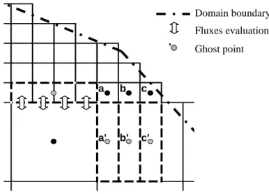
The space discretization of Eq. (1) is performed by means of a finite volume scheme. This ensures a proper mass and momentum conservation, which is a prerequisite for handling reliably discontinuous solutions such as moving hydraulic jumps. As a consequence, no assumption is required as regards the smoothness of the solution. Reconstruction at cells interfaces can be performed constantly or linearly, in conjunction with slope limiting, leading in the second case to a second-order spatial accuracy. In a similar way, variables at the border between adjacent blocks are reconstructed linearly, using in addition ghost points as depicted in Figure 1. The variables at the ghost points are evaluated from the value of the subjacent cells. Moreover, to ensure conservation properties at the border between adjacent blocks and thus to compute accurate volume and momentum balances, fluxes related to the larger cells are computed at the level of the finer ones.

a b c

a' b' c'

Domain boundary Fluxes evaluation

’ _{Ghost point}

Figure 1: Border between two adjacent blocks on a Cartesian multiblock grid

Appropriate flux computation has always been a challenging issue in computational fluid dynamics. The fluxes f and g are computed by a Flux Vector Splitting (FVS) method developed by the authors. Following this FVS, the upwinding direction of each term of the fluxes is simply dictated by the sign of the flow velocity reconstructed at the cells interfaces. It can be formally expressed as follows:

2 2 0 ; 2 0 hu hu gh huv + − ⎛ ⎞ ⎛ ⎜ ⎟ ⎜ =_{⎜ ⎟} =_⎜ ⎜ ⎟ ⎜ ⎝ ⎠ ⎝ f f ⎞ ⎟ ⎟ ⎟ ⎠ and 2 2 0 ; 0 2 hv huv hv gh + − ⎛ ⎞ ⎛ ⎜ ⎟ ⎜ =_{⎜ ⎟} =_⎜ ⎜ ⎟ ⎜ ⎝ ⎠ ⎝ ⎞ ⎟ ⎟ ⎟ ⎠ g g , (6)

where the exponents + and – refer to, respectively, an upstream and a downstream evaluation of the corresponding terms. A Von Neumann stability analysis has demonstrated that this FVS leads to a stable spatial discretization of the terms ∂ ∂f x and ∂ ∂g y in Eq. (1) [3]. Due to their diffusive nature, the fluxes

fd and gd are legitimately evaluated by means of a centred scheme.

Besides requiring a low computation cost, this FVS offers the advantages of being completely Froude independent and of facilitating a satisfactory adequacy with the discretization of the bottom slope term. This FVS has already proved its validity and efficiency for numerous applications [3, 4, 5, 6, 7].

2.4 Topography

gradients

The discretization of the topography gradients is also a challenging task when setting up a numerical flow solver based on the SWE. The bed slope appears as a source term in the momentum equations. As a driving force of the flow, it has however to be discretized carefully, in particular regarding the treatment of the advective terms leading to the water movement, such as pressure and momentum.

In the model presented in this paper, according to the FVS characteristics, a suitable treatment of the topography gradient source term of Eq. 4 is a downstream discretization of the bottom slope and a mean evaluation of the corresponding water heights [4]. For a mesh i and considering a constant reconstruction of the variables, the bottom slope discretization writes:

(

1

) (

1

)

, 2 , b b i i i b i h h z z z gh g x y x y + + ∂ + − ∂ − → − ∂ ∂ i (7) where subscript i+1 refers to the downstream mesh along x- or y- axis.

This approach fulfils the numerical compatibility conditions defined by Nujic [8] regarding the stability of water at rest. The final formulation is the same as the one proposed by Soares Frazão [9] or Audusse [10]. It is suited to be used in both 1D and 2D models, along x- and y- axis. Its very light expression benefits directly from the simplicity of the original spatial discretization scheme.

Nevertheless, the formulation of Eq. (7) constitutes only a first step towards an adequate form of the topography gradient as it is not entirely suited regarding water in movement over an irregular bed. The effect of kinetic terms is not taken into account and, as a consequence, inaccurate evaluation of the flow energy evolution can occur when modelling flow over a variable topography [4].

2.5 Time discretization and boundary conditions

Since the model is applied to transient flows and flood waves, the time integration is performed by means of a second order accurate and hardly dissipative explicit Runge-Kutta (RK) method. For stability reasons, the time step is constrained by the Courant-Friedrichs-Levy (CFL) condition based on gravity waves. A semi-implicit treatment of the bottom friction term is used, without requiring additional computational costs.

For each application, the value of the specific discharge can be prescribed as an inflow boundary condition. Besides, the transverse specific discharge is usually set to zero at the inflow even if its value can also be prescribed to a different value if necessary. In case of supercritical flow, a water elevation can be provided as additional inflow boundary condition. The outflow boundary condition may be a water surface elevation, a Froude number or no specific condition if the outflow is supercritical. At solid walls, the component of the specific discharge normal to the wall is set to zero. In case of dam break flow modelling, no boundary condition is generally needed in the model as the flows in the reservoir and the downstream valley are bounded by the natural topography.

3 Model

validation

The first test case consists in computing the flow induced by the instantaneous collapse of an idealized circular dam, as initially described by Alcrudo [11]. A cylindrical dam with radius equal to 11 m is considered, separating the computational domain into an inner and an external area, with respective initial water depths of 10 m and 1 m, and zero discharge. The bed is horizontal, while the bed friction and viscosity are neglected. The dam is removed at time t = 0.

Since the problem is actually one-dimensional along the radial direction, a reference solution obtained from a 1D computation on a very fine grid may be used to compare with the results of the 2D simulations. The test case enables to verify, on one hand, the ability of the model to represent the two-dimensional propagation of unsteady stiff waves and, on the other hand, to check the capacity of the model to preserve symmetry within the numerical solution.

The reference solution is obtained by solving the 1D formulation of the continuity and momentum equations, written as a function of a radial coordinate and considering the rotational symmetry [3]. The system has been solved on a fine mesh (2,000 elements), based on a finite volume scheme second-order accurate both in space and time (RK22 and linear reconstruction with slope limitation).

Two-dimensional simulations have been conducted on a single block with cells of 0.25 m, as well as on a finer mesh (0.10 m cells). The time integration is performed with the same numerical scheme.

Figure 2 illustrates the free surface obtained at four successive times. The solution involves a shock propagating towards outside and a rarefaction wave propagating towards inside. It must be noted that, in contrast with the Stoker solution, the part of the solution immediately upstream of the shock is not a horizontal platform anymore, as a result of the two-dimensional behaviour of the flow.

(a) (b) (c) (d)

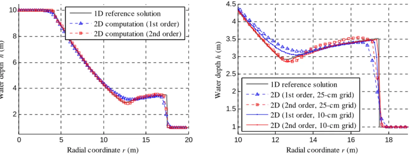
Figure 2: Instantaneous 3D views of the free surface at four different time steps following the instantaneous collapse of an idealized circular dam: (a) 0 s, (b) 0.20 s, (c) 0.40 s and (d) 0.69 s. Figure 3 shows the satisfactory agreement between the radial distributions of water depth in the reference solution and the one predicted by the computation. For comparison purpose, the 2D simulations have been conducted with either a first or a second order accurate space discretization. The overall shock propagation is faithfully reproduced by both schemes, while the second-order scheme achieves slightly better results at both sides of the rarefaction wave as well as in the vicinity of the shock, as a result of its weaker numerical diffusion. Although refining the grid obviously contributes to improve the solution, the second-order space discretization on the 0.25 m mesh performs almost as well as it does on the finer mesh.

0 5 10 15 20 2 4 6 8 10 Radial coordinate r (m) W at er de pt h h (m ) 1D reference solution 2D computation (1st order) 2D computation (2nd order) 10 12 14 16 18 1 1.5 2 2.5 3 3.5 4 4.5 Radial coordinate r (m) W at er de pt h h (m ) 1D reference solution 2D (1st order, 25-cm grid) 2D (2nd order, 25-cm grid) 2D (1st order, 10-cm grid) 2D (2nd order, 10-cm grid)

Figure 3: Computed water depths after 0.69 s for the flow induced by the collapse of a circular dam. 1D reference solution as well as 2D solutions obtained with schemes first and second order accurate in

Different authors have studied the circular dam-break problem on structured polar grids [11, 12], which enable to preserve the cylindrical symmetry of the solution. In contrast, computations performed on Cartesian grids show some influence of the axes of reference on the waves propagation [11, 12] and simulations based on unstructured grids, such as triangular cells, are unable to preserve the cylindrical symmetry [13]. In the present case, the contourlines displayed in Figure 4(a) demonstrate the correct global reproduction of the symmetry of the flow, while Figure 4(b) highlights precisely the achieved rotational symmetry of order four, which is actually the best level of symmetry possible to be reached exactly on a Cartesian grid.

(a) -20 -15 -10 -5 0 5 10 15 20 -20 -15 -10 -5 0 5 10 15 20 1 1 1 11 1 1 1 1 1 1 2 2 ₂ 2 2 2 2 2 3 3 3 3 3 3 3 3 4 4 4 4 4 5 5 5 5 6 6 6 6 7 7 7 8 8 8 9 9 (b) -20 -15 -10 -5 0 5 10 15 20 -20 -15 -10 -5 0 5 10 15 20 1 1 1 11 1 1 1 1 1 1 1.1 1.1 1.1 1.1 1.1 1.1 1.1 1 .1 3.2 5 3.25 3.25 3 .2 5 3.25 3.25 3.25 3.2 5 3.25 3.25 3.25 3.25 3.2₅ 3.25 3.25 3.25 3.2₅ 3.25 3.25 3 .2 5 3.5 3.5 3.5 3.5 3.5 5 5 5 5 6 6 6 6 7 7 7 8 8 8 9 9

Figure 4: Contourlines of the free surface (m) after 0.69 s for the flow induced by the circular dam break. (a) Uniform distribution of the contourlines and (b) detail of the variations close to the shock.

3.2 Dam break in a L-channel

To assess the efficiency of the numerical model to compute dam break induced waves in non straight channels, the L-channel experimental benchmark of the European CADAM Project [14, 15] has been considered as a second validation example.

Elevation 2 cm square meshes 6 cm square meshes Plane view

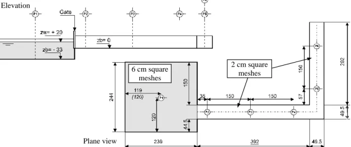
Figure 5: Experimental facility for the L-channel test (dimensions in cm) and numerical discretization features

The experimental facility consists in a square reservoir upstream of two rough horizontal channel reaches linked by a 90° bend (Fig. 5). The channel cross section is rectangular. The downstream reach extremity is a free chute. A 33 cm high topography step is located between the reservoir and the first reach. A guillotine type gate separates the reservoir and the channel. At time zero, the gate is almost instantaneously lifted and a wave propagates into the channel reaches, with partial reflection on the 90° bend. The experimental facility is equipped with 6 gauges measuring the water depth evolution during 20 s with a frequency of 0.1 s.

Preliminary numerical tests suggested a roughness coefficient equal to

0.006 s/m

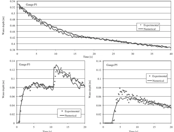
1/3 for both the steel bottom and the glass side walls. The simulation has been performed with a first order accurate space discretization scheme (even across block boundaries) and a second order accurate time integration scheme (RK 22 – CFL = 0.1). The grid for numerical modelling is based on 2 cm square meshes in the channel reaches and 6 cm ones in the reservoir (Fig. 5).

The curves of Figure 6 show the unsteady evolution of the water depths in the reservoir and the channel reaches at gauges 1, 3 and 5 in both the experimental facility and the numerical model. The numerical results are in very good agreement with the experimental ones.

0.38 0.4 0.42 0.44 0.46 0.48 0.5 0.52 0.54 0 5 10 15 20 25 30 35 40 W a te r de pt h [ m ] Time [s] Gauge P1 Experimental Numerical 0 0.02 0.04 0.06 0.08 0.1 0.12 0.14 0 5 10 15 20 W a te r d e pt h [ m ] Time [s] Gauge P3 Experimental Numerical 0 0.02 0.04 0.06 0.08 0.1 0.12 0.14 0 5 10 15 20 W a te r dep th [m ] Time [s] Gauge P5 Experimental Numerical

Figure 6: Comparison of experimental and computed water depths evolution in the L-channel.

3.4 Malpasset

dam

break

As it is well documented, the dramatic real dam break case of the Malpasset 66-m high arch-dam in France (2nd December 1959) has been used as a benchmark in the frame of the CADAM project [14]. Wave propagation times are available since exact shutdown times are known for three electric transformers destroyed by the wave induced by the sudden and total collapse of the dam. In addition, a survey conducted by the police showed the highest water marks on both left and right banks of the downstream 12-km long Reyran valley. Furthermore, a non-distorted 1/400 scale model was built in 1964

by EDF, the former owner of the dam and member of CADAM group, and was calibrated against field measurements. It provided supplementary water levels and propagation time data [16].

Topographic information has been generated by interpolation from maps of the National Geographical Institute. Elevation of the valley ranges from minus 20 m at the sea bottom up to 100 m, this latter being the estimated initial free surface level in the reservoir (with an uncertainty of about 50 cm). From physical scale model tests, the Manning roughness has been estimated to be 0.0286 s/m1/3. Upstream of the reservoir, the inlet discharge is assumed to be null.

The numerical model discretization sketch is defined as on Figure 7 [5]. No boundary conditions are needed since the topography is high enough to include a dry strip all around the computation domain. In the sea, the free surface water level is assumed to be constant at 0 m. Initially, the dam is defined as a straight line between two points, with a reservoir at constant level. Except in the reservoir and in the sea, the computation domain is dry. The simulations have been carried out with a RK 22 time scheme and a CFL number equal to 0.1.

(b) (a)

Figure 7: Blocks definition on shaded view of the topography (m) (a) and comparison of the flood extension, represented with maximum water depths (m), according to the police survey points (b) Figure 8 shows the satisfactory comparison between computed results and the field and laboratory measurements. Marks A to C designate the 3 electric transformers. Since transformer A is located in the bottom of the valley, its shutdown time is the wave arrival time. For the two others, as the shutdown time is supposed to be between wave arrival time and time of maximum water level, it is more relevant to compare the time interval between shutdowns. Regarding topography precision, maximum water levels are satisfactory in comparison with measurement points (Figure 8). The map of the maximum water depths (Fig. 7) corroborates again the good results of the simulation regarding flood extension, in comparison with the police survey points.

A B C S6 S7 S8 S9 S10 S11 S12 S13 S14 (a) 0 _(b) 200 400 600 800 1000 1200 1400 1600 Ti m e ( s) Real event Numerical P1 P2 P3 P4 P5 P6 P7 P8 P9 P10 P11 P12 P15 P17 S6 S7 S8 S9 S10 S11 S12 S13 S14 0 10 20 30 40 50 60 70 80 90 100 F re e s u rf ace e levat ion (m ) Real event Numerical

Figure 8: Wave arrival times to electric transformers (A to C) and physical model gauges (S6 to S14) (a) and maximum water levels at police survey points (P1 to P17) and at physical model gauges (b)

4 Application using high resolution DEM

A few years ago, the Walloon Ministry of Facilities and Transport (MET) of Belgium acquired an accurate DEM covering a large part of the hydrographic network in the South of the country. An airborne laser has been used to measure the topography of the floodplain of the main rivers network and an echo-sonar technique has been applied to characterise the bathymetry of the main channel on navigable rivers. Consequently, the poor and inaccurate topography information available for many years, i.e. 30 m of plan resolution with a weak precision in elevation, has been replaced by an exceptional data set since the laser and sonar precision in altitude is 15 cm and the information density is one point per square meter. Regarding flow computations, scientific work has demonstrated that this huge improvement in the quality of the main data set enables to focus on proper physical values of the roughness coefficient rather than using it to assess the effect of blockage by buildings or of large irregularities of the topography. It allows also refining the hydrodynamics computations at the scale of houses and streets [7].

The hydrodynamic model presented in this paper has been applied, using this high resolution DEM, to produce hazard maps downstream of Belgian large dams in the framework of a complete risk analysis. In this scope, after the definition of specific failure scenarios for each dam, global transient 2D simulations have been carried out to assess the wave propagation in the reservoirs and in the downstream valleys. The simulation meshes were based on grids of about 1,000,000 potential computation cells. The results enable to plot essential hazard maps (time of arrival of the front, maximum water depths and unit discharges) as well as hydrographs and limnigraphs at a number of strategic points downstream of the dams (urbanized areas, bridges, …), which constitute key input for the subsequent stages of the risk analysis process [17]. The refinement of these results in urban area is illustrated on Figure 9.

(a)

(b)

Figure 9: Instantaneous views of the water depths (a) and field of unit discharges (b) in an urban area downstream of a dam break.

5 Conclusion

Depth-averaged hydrodynamic models constitute a realistic numerical approach for accurate and finely distributed computation of dam-break wave propagation. Such a model is presented in details in this paper. Its particular features enable a stable and accurate flow computation, even on irregular wetting-drying topography, with an exact conservation of the mass and momentum quantities. It is also able to deal with large grids, up to 1,000,000 meshes, without leading to prohibitive computation times. Following extensive validation by comparison with theoretical, experimental and field data, the 2D model

application to real cases, in combination with high resolution DEM, provides entry data of prime interest for EAP setting at the scale of houses and streets.

More recently, theoretical and experimental investigations have been initiated with the purpose of a better understanding of the interactions between the flood wave and the buildings or other structures present in the downstream valley. Based on a process-oriented analysis, the scope of the research is to identify the criteria for failure of those buildings and to take it into account in the flow simulations.

References

[1] M. Pirotton. Modélisation des discontinuités en écoulement instationnaire à surface libre. Du ruissellement hydrologique en fine lame à la propagation d’ondes consécutives aux ruptures de barrages. PhD Thesis, University of Liege, 1994

[2] J-M Hervouet. Hydrodynamique des écoulements à surface libre – Modélisation numérique avec la méthode des éléments finis. Presses de l’école nationale des Ponts et Chaussées : Paris, 2003.

[3] B.J. Dewals. Une approche unifiée pour la modélisation d'écoulements à surface libre, de leur effet érosif sur une structure et de leur interaction avec divers constituants. PhD thesis, University of

Liege, 2006

[4] S. Erpicum. Optimisation objective de paramètres en écoulements turbulents à surface libre sur maillage multibloc. PhD thesis, University of Liege, 2006

[5] S. Erpicum, P. Archambeau, B.J. Dewals, S. Detrembleur, C. Fraikin and M. Pirotton. Computation of the Malpasset dam break with a 2D conservative flow solver on a multiblock structured grid. In Liong, Phoon and Babovic, editors, Proc. of 6th Int. Conf. on Hydroinformatics, Singapore, 2004

[6] P. Archambeau. Contribution à la modélisation de la genèse et de la propagation des crues et inondations. PhD thesis, University of Liege, 2006

[7] S. Erpicum, B.J. Dewals, P. Archambeau, S. Detrembleur and M. Pirotton. Detailed 2D numerical modeling for flood extension forecasting. Riverflow’08 , Izmir, Turkey, 2008 (Accepted)

[8] M. Nujic. Efficient implementation of non-oscillatory schemes for the computation of free surface flows. Journal of Hydraulic Research. 33(1):101-111, 1995

[9] S. Soares Frazão. Dam-break induced flows in complex topographies – Theoretical, numerical and

experimental approaches. PhD Thesis, Université Catholique de Louvain, 2000

[10] E. Audusse. Modélisation hyperbolique et analyse numérique pour les écoulements en eaux peu profondes. PhD thesis, Université Paris VI – Pierre et Marie Curie, 2004.

[11] F. Alcrudo and P. Garcia-Navarro. A high resolution Godunov-type scheme in finite volumes for the 2D shallow-water equations. Int. J. for Numerical Methods in Fluids, 16: 489-505, 1993

[12] C. Mingham and D. Causon, High-resolution finite volume method for shallow water flows. J. of

Hydraulic Engineering - ASCE, 124(6):605-614, 1998

[13] K. Anastasiou and C. Chan, Solution of the 2D shallow water equations using finite volume method on unstructured triangular meshes. Int. J. for Numerical Methods in Fluids, 24:1225-1245, 1997 [14] M. Morris, CADAM – Final report. European Commission, 2000

[15] S. Soares Frazão, X. Sillen and Y. Zech. Dam-break flow through sharp bends – Physical model and 2D Boltzmann model validation. In Proc. of CADAM Wallingford Meeting, Wallingford, 1998 [16] N. Goutal. The Malpasset dam failure. An overview and test case definition. In Proc. of CADAM

Zaragoza meeting, Zaragoza, 1999

[17] B.J. Dewals, S. Erpicum, P. Archambeau, S. Detrembleur and M. Pirotton, Numerical tools for dam break risk assessment: validation and application to a large complex of dams, in Improvements in

reservoir construction, operation and maintenance, H. Hewlett, editor, Thomas Telford: London,