Family Income and Child Outcomes: The 1990 Cocoa Price Shock in Cote d’Ivoire

(1)

D

OCUMENT DE

T

RAVAIL

DT/2008-05

Family Income and Child

Outcomes: The 1990 Cocoa Price

Shock in Cote d’Ivoire

Denis COGNEAU

Rémi JEDWAB

(2)

List of Figures

Figure 1: National Cocoa Producer Prices and Average Per Capita Consumption forCocoa Producers and Non-Cocoa Farmers ... 25

Figure 2: Kernel Density of the Share of Cocoa Producers Within Villages where this Share is Positive ... 25

Figure 3: Average Cocoa Production by District in 1987-1988-1989 and Occupational Specialization of Surveyed Villages in 1986-1988 and 1993 ... 26

Figure 4: Difference-in-Difference in Income CDFs for 5-11 y.o. Children... 27

Figure 5: Actual and Simulated (Uniform Shock) Difference-in-Difference in Income CDFs for 5-11 y.o. Children ... 27

List of Tables

Table 1: Results for the Reduced-Form Model, School Enrollment (School 5-11), Child Labor ... 28

Table 2: Mean Characteristics for 2-15 y.o. Children for Cocoa Producers and Non- Cocoa Farmers, in 1988 ... 29

Table 3: Relative 1988-1993 Change in Observables for 2-15 y.o. Children between Cocoa Producers and Non-Cocoa Farmers ... 29

Table 4: IV1 and IV2 Second-Stage and First-Stage Results for School Enrollment, 5-11 y.o. Children ... 30

Table 5: Results for School Enrollment (School 5-11), Child Labor (Work 9-15), Heightfor- Age Z-score (HAZ 2-5), and Health Status (Sick 2-15) ... 31

Table 6: IV1 Results for School Enrollment (School 5-11), Child Labor (Work 9-15), Height-for-Age Z-score (HAZ 2-5) and Health Status (Sick 2-15) according to the Spatial ... 32

(3)

Family Income and Child Outcomes: The 1990

Cocoa Price Shock in Cote d’Ivoire

∗

Denis Cogneau

†

R´

emi Jedwab

‡

Draft Version: July 17th 2008

Abstract

We study the drastic cut of the administered cocoa producer price in 1990 Cote d’Ivoire and investigate the extent to which cocoa producers’ children suffered from this severe income shock in terms of school enrollment, increased labor, height stature and sickness. Comparing pre-crisis (1986-1988) data and post-crisis (1993) data, we propose a difference-in-difference within-village strategy in order to identify the causal effect of family income on children outcomes. We find a strong impact of family income variation for the four variables we examine.

Keywords: Education, Health, Child Labor, Development. JEL classification codes: I12, I21, 012

∗_{We thank the Ivorian National Institute for Statistics for giving us access to the surveys.} We also thank Michael Grimm, Marc Gurgand, Sylvie Lambert and Thomas Piketty for help-ful discussions and suggestions, and seminar participants at Oxford (CSAE), London (Brunel), Stockholm, Clermont-Ferrand (CERDI) and Paris (PSE). The usual disclaimer applies.

†_{Corresponding author.} _{IRD, DIAL and Paris School of Economics (INRA). Paris} School of Economics, 48 boulevard Jourdan - 75014 Paris. Tel: +33143136373. E-mail: cogneau@dial.prd.fr

(4)

Family Income and Child Outcomes: The 1990 Cocoa Price Shock in Cote d’Ivoire

Abstract

We study the drastic cut of the administered cocoa producer price in 1990 Cote d’Ivoire and investigate the extent to which cocoa producers’ children suffered from this severe income shock in terms of school enrollment, increased labor, height stature and sickness. Comparing pre-crisis (1986-1988) data and post-crisis (1993) data, we propose a difference-in-difference within-village strategy in order to identify the causal effect of family income on children outcomes. We find a strong impact of family income variation for the four variables we examine.

1 Introduction

In many low-income countries and in Africa in particular, performances with re-gard to child education and health are still very much disappointing (see Appendix 1). While the disease-prone environment and the low availability and quality of infrastructures bear a large responsibility in this situation, on the demand side low parental resources also constitute a direct limiting factor. A large body of econo-metric works has already addressed the issue of estimating the impact of parental income on child outcomes in developing countries. This literature has long recog-nized that the statistical correlations between these two latter variables are merely an indirect and potentially biased reflection of the causal impact of income (see, e.g., Blau 1999; Behrman and Knowles 1999). One reason is the contamination of income indicators by relatively large measurement errors or idiosyncratic tran-sient components. Another reason is the possible endogeneity of parental income due to omitted variables: Some unobservable preferences and resources may si-multaneously determine parental income, child work, child schooling, and child care.

Randomized experiments are a first answer to this endogeneity problem. The evaluations of the famous Mexican conditional cash transfer program Progresa

(5)

have revealed a strong and causal sensitivity of school enrollment to the transfers delivered to families that send their children to school (e.g., Schultz, 2004; De Janvry and al. 2004). However, the impacts of unconditional income variations and of negative income shocks, the impacts on other outcomes than schooling such as health, and the influence of the socioeconomic context (e.g. Africa vis-a-vis Latin America) are still not well known. In the absence of randomized experiments, a bunch of recent works exploits the income variability generated by macroeconomic crises (Thomas and al., 2004), commodity price changes (Edmonds and Pavcnik 2005; Kruger, 2007), shocks on production (Jensen, 2000; Beegle, Dehejia and Gatti, 2006; Banerjee et al., 2007) or targeted policy reforms (like that of the South-African pension-system: Duflo 2000 and 2003; Case, 2001; Edmonds 2006) in a variety of contexts. Many of these works suggest that income has direct and large effects on child outcomes, and are suggestive of the strong liquidity constraints that weight on poor households (with the exception of Kruger, op.cit., in the case of child labor in Brazil).

Our work pertains to this family. We study the drastic cut of the adminis-tered cocoa producer price in 1990 Cote d’Ivoire and look at the extent to which cocoa producers’ children suffered from this severe income shock in terms of school enrollment, increased labor, height stature and sickness. Cote d’Ivoire is the world leading exporter of cocoa beans. In the period 1985-1994, cocoa beans exports amounted to more than one third of Ivorian total exports; as such, the Cote d’Ivoire economy was and still is highly dependent on cocoa international prices. As those latter were plummeting over the 1980s, the parastatal marketing board finally decided to halve the producer price in 1990, from 400 to 200 CFA francs per kilogram. We exploit two datasets from nationally representative large sam-ple household surveys that were imsam-plemented before and after the cocoa crisis, in 1986-89 and 1992-93 respectively.

We implement two kinds of identification strategies of the impact of income shocks. Our preferred strategy is a double difference, whereby we compare the

(6)

evolution of outcomes of children living in cocoa producing households with that of children living in other agricultural households. We even compare children living in the same villages, in order to absorb the potential variation in supply-side factors. Of course, given the weight of cocoa production in the Cote d’Ivoire economy, the comparison group (non-cocoa farmers’ children) is also affected by the cocoa crisis, so that we do not measure the overall impact of the cocoa crisis but only use it in order to identify the causal impact of a negative private income shock. A second identification strategy exploits the weight of cocoa production in the district of birth of the children, in keeping with previous works that also rely on regional variation (Jensen, 2000; Kruger, 2007; Banerjee et al., 2007). This second strategy offers results that are broadly consistent with the first; Income matters as regards parental decisions to invest in the health and education of their children.

The remainder of this paper is organized as follows. Section 2 proposes a very simple theoretical model of school enrollment that illustrates the main endogeneity bias that may affect the econometric estimation of the causal impact of household income on children outcomes. Section 3 presents the data and the construction of the main variables. Section 4 describes the socioeconomic context of the natural experiment and some suggestive descriptive statistics about the long-term consequences of the cocoa shock. Section 5 presents our two double-difference identification strategies. Section 6 examines the assumptions that underlie the validity of our identification strategies and provides supportive evidence in their favor. Section 7 presents the results. Section 8 discusses distinct aspects of our results regarding the influence of the local context. Section 9 summarizes and concludes.

2 Theoretical Framework and Identification Issues

We here write the simplest microeconomic model of school enrollment decision, in order to raise the main identification questions that we have to solve out. A child

(7)

care model (including nutrition and medical expenditures) could be devised the same way. Let us consider families (indexed by i) which have to decide whether they send their children to school (Si = 1) or not (Si = 0), depending on their

ability to pay the costs of schooling (γi) and on the impact of the schooling decision

on their utility. Parents determine the allocation of their permanent income (Yi)

between consumption (Ci) and schooling in order to maximize a utility function

U (Ci, Si). The maximization is performed subject to a budget constraint Ci +

γiSi = Yi. Assuming that U is concave and additively separable (U (Ci, Si) =

C_iα+ βiSi) and that γi remains small with respect to Yi, it is not difficult to check

that: Si = 1 ⇐⇒ U (Yi − γi, 1) > U (Yi, 0) ⇐⇒ ln Yi > 1 1 − αln αγi βi ! (1)

Parents send their children to school if and only if their income is sufficiently high for the impact of schooling cost on family consumption to be small enough. One straightforward extension of this school enrollment model is to assume that the net cost γi/βi depends on the characteristics of the child and that the parental

decision is taken in two steps: in a first step, they evaluate the optimal timing of their children’s schooling (i.e., the timing that minimizes γi/βi) and, in a second

step, they choose to send or not their children to school depending on whether condition (1) holds true or not. In particular, we will consider that the optimal timing is not necessarily the same for cocoa producers compared to other farmers. It should however be acknowledged that such a model is more adapted to explaining delayed entry, i.e. the probability of not being schooled on time (at 5 years old, at the first compulsory primary level called CP1) or at any age conditional on a given timing. It is less suited to explaining school dropouts, as the model should then be dynamic and include past school experience into the net cost of school enrollment. However, the data will not allow us to distinguish late entries and early drop-outs, unlike Bommier and Lambert (2002), as the age of entry into school and

(8)

the school curriculum of children are not available. Moreover, dynamic models raise identification difficulties that are rather difficult to overcome (Cameron and Heckman, 1998). Therefore, we will simply analyze the probability of attending school in a given year and relate it to the household current income, but will consider the heterogeneity of the income treatment with respect to such observable variables as the age of children, as well as to their gender, relation to the household head and birth order. To specify our empirical models, we will assume that the net cost γi/βi of schooling can be expressed as a linear function of (a) the child’s

exogenous characteristics Xi such as her/his gender and age, (b) head’s education

and other household characteristics Hi, (c) location characteristics Vi, and (d)

child or household unobservable determinants εi.

Si = I(aYi+ Xib1+ Hib2+ Vi+ εi > 0) (2)

where I(x > 0) is a dummy that takes the value 1 whenever x is positive. From an econometric point of view, the main problem for estimating (2) is the potential en-dogeneity of income, parental education and some other household characteristics. In this paper, we are only interested in the estimation of the causal effect of the former. The reasons for such endogeneity of income are the classical simultaneity, omission and measurement errors biases. A first example of simultaneity bias is the fact that child schooling and household income are jointly determined through the decision regarding child labor; in other words, the more a child works, the lower his/her schooling enrollment but the higher the total household income (downward bias). Another omission bias is income being correlated with unobserved parental abilities and parental preferences towards education, which could either positively influence child schooling (upward bias) or else negatively (downward bias) if skilled parents put their children to work early in order to transmit their savoir-faire. Be-sides, richer parents may locate in villages with a better school (Vi), thus implying

a relatively lower net cost γi/βi (upward bias). Lastly, our measure of income

(9)

bias). Therefore, the identification of our model requires the construction of in-strumental variables which are correlated with household income but uncorrelated with unobserved family-specific factors and measurement errors.

3 Data

Our main sources of data are three Cote d’Ivoire Living Standards Surveys (CILSS) from 1986 to 1988, and the Enquˆete Prioritaire (EP) 1993, conducted by the Institut National de la Statistique of Cote d’Ivoire with the support of the World Bank. As we are only interested in the comparison of children between the pre-crisis and the post-pre-crisis period, we stack all the household data for 1986-1988 and label them 1988.

Regarding children outcomes, the surveys ask the same questions about school enrollment and child work during the previous year. Our definition of child work includes child labor on domestic farms and in domestic businesses, but not household chores since there are no related data. As already noted, the surveys unfortunately do not provide details on the children school curriculum nor on age of entry into school.1 With respect to health outcomes, the questions about sick-ness episodes during the preceding month are the same, and height and weight are measured for every child between 6 months and 5 years. We can then construct height-for-age Z-scores following the procedure recommended by the World Health Organization.2

In each of the two datasets, we are able to define in an homogeneous way the

1_{Moreover, the question ”Have you ever been at school?” that is asked in 1993 is formulated} in a much wider manner in 1988 as ”Have you ever followed any kind of training?” and thus includes apprenticeship and koranic schools. Likewise, level attained can not be used as informal curricula are not distinguished. The questions on literacy are not comparable either as the ability of reading and writing is asked without any precision in 1993, whereas it is characterized as the capacity to read a newspaper and write a letter in 1988.

2_{See WHO Multicentre Growth Reference Study Group (2006). Details of such calculations} are available on the Internet WHO website: http://www.who.int/childgrowth/software/en/

(10)

group of cocoa producing households, whether they are landowners with tenants who grow cocoa trees, or landowners or sharecroppers who directly collect cocoa (at least 1 kg within the year). As the district (”d´epartement”) of birth is available in each survey, we are also able to know whether a child was born in a cocoa-producing district or not.

Our preferred income variable is consumption per capita at 1988 prices; con-sumption is much better measured than income in that kind of surveys (see e.g. Deaton, 1997). Our consumption concept includes consumption of own food pro-duction, and all cash expenditures including an imputed housing rent, but exclud-ing very infrequent durable goods acquisition and health expenditures.3 _Income

available for consumption corresponds to the ex-post income obtained once coping strategies have been implemented to mitigate the ex-ante cocoa income cut: in-crease in labor supply, dissaving and sale of assets, borrowing, etc. Despite these coping strategies, what follows will show that liquidity constraints still weight heavily on the welfare of the children.

4 The Cocoa Shock

So as to solve income endogeneity, we use the natural experiment provided by the exogenous changes in cocoa producer prices in Cote d’Ivoire over the period 1986-1993. From independence till the mid-1970’s, Cote d’Ivoire has experienced dramatic growth thanks to the development of cocoa exports in a context of ris-ing primary commodity prices. Migration from Northern regions and neighborris-ing countries (Burkina-Faso and Mali) was encouraged in order to provide the neces-sary workforce to this expanding sector. The expansion of production also relied on the extensive exploitation of new forest areas in the South-Western part of the country. The producer price was administered by the state-owned marketing board

3_{We also used the cash expenditures variable excluding consumption of own food production,} knowing that the cocoa income loss directly affects cash income. The results obtained with this latter are largely consistent with those obtained with total consumption.

(11)

(the ”Caisstab”), which fixed it much below the international price: for instance, over the period 1974-1980, the producer price only represented 45% of the export price. The benefits of the Caisstab constituted extra-budgetary resources which were extensively used to finance the fiscal deficit, aside to the taxes also levied on cocoa exports. This allowed the Ivorian government to pay high wages to its skilled civil servants and to fund a wide expansion of the education sector (Azam, 1993). Starting from a very low colonial level, Cote d’Ivoire managed to catch up with the neighboring Ghana where the British colonial ruler had much more developed education. From 1979, the decline in international cocoa prices and the subsequent increasing deficits of the Caisstab designated the end of the ”Ivorian Miracle”. Many public investments that had been financed through international debt proved to be at the same time not very efficient. Cote d’Ivoire progres-sively entered in a period of financial crisis and adjustment that would last almost twenty years (Berth´elemy and Bourguignon, 1996; Cogneau and Mespl´e-Somps, 2003). After a short-lived rebound in 1985-1986, and despite a governmental at-tempt to influence international cocoa prices by rationing cocoa exports in 1987, those latter kept falling. In June 1989, the cocoa producer price was abruptly cut for the first time in 25 years, first from 400 to 250 CFA francs per kilogram; then in 1990, it was purely halved to 200 CFA francs. In 1994, a new rebound of international prices, combined with the CFA franc devaluation, authorized to increase at new the producer price. In 1998, the Caisstab was dismantled and the cocoa trade liberalized. But this is another story (Grimm, 2004).

Between 1986 and 1993, we expect cocoa-producers’ income to have fallen much more than the rest of the population. In particular, 1986, 1987 and 1988 have been years of high yields and high prices for cocoa producers while they were years of low yields and low prices for coffee producers, and years of low prices for staple food producers (Jones and Ye, 1997). After 1990, yields remained high for cocoa producers, while the prices of other agricultural products remained stable. In order to examine the income consequences of the shock, we define a

(12)

treatment group, the sample of cocoa-producing households (whether landowner or tenant, as already stated above), and a comparison group, the sample of non-cocoa agricultural households (defined as being households whose head is a farmer but do not produce cocoa at all). Even if we work with the whole national sample in order for our two IV strategies to be comparable (see thereafter), we set aside non-agricultural households by including specific dummies for them. Figure 1 confirms that cocoa households’ average income has fallen more than the one of their non-cocoa agricultural counterparts, by 36% against 24%, although each category has been very much affected by the cocoa-induced macroeconomic crisis.4

We now look at whether cocoa households have comparatively more de-creased their investments in their offspring’s health or education. In the case of education, let us first point out that assessing the long-term consequences of the cocoa shock turns out to be difficult. Indeed, the data does not allow tracing back the type of household (cocoa vs. non-cocoa) where an adult individual actually lived at school age years. This precludes comparing definitive educational attain-ments (literacy, completed primary level) between treated adults and non-treated adults. In the case of health however, average differences in height-for-age deficits mirror the past investments in child care from the parents and the quantity and quality of nutrition received, especially at very young ages (Martorell and Habicht, 1986). In particular, a height-for-age Z-score lower than -2 means that a child has experienced a severe growth failure, and this kind of accident is widely considered as a health handicap in adult age. We actually focus on the analysis of height stature on 2-5 year-old children. First, we only have anthropometric data from 6 months to 5. Second, it can be argued that differences that are due to distinct investments between 0 and 2 usually better show up at ages 2-5 (Moradi 2006).

Table 1 anticipates on econometric results and presents the double differences

4_{For the whole sample, our estimated consumption per capita loss between 1986-88 and 1993} amounts to 28%, which is consistent with estimates from Maddison (2003) indicating a 27% fall of real GDP per capita.

(13)

of children outcomes and household income that we shall exploit later on. It shows that in 1993 the situation of children living in cocoa households has significantly deteriorated in comparison with children living in other farming households: they are less often enrolled at school and more often working, they have become rela-tively smaller and are more often declared as sick. The two figures about schooling and stunting suggest that the cocoa price shock might have had very serious con-sequences on the capabilities of the children living in cocoa-producing districts or cocoa-producing households. Although we can not definitively prove it, it is fairly possible that some minimal education was not received and could not be recovered; the same holds for the small stature inherited from stunting in that it reflects an irreversibly diminished health capital. The cohorts who were the most at risk in terms of primary education or nutrition and health care in the beginning 1990s could be doomed to carry all along their life the handicaps brought about by this unfavorable period. It remains to be checked whether the parental income channel can credibly explain these long-term consequences.

Before focusing on this channel, it is worth pointing out that the cocoa price shock had potentially two distinct effects: one was to decrease the returns to cocoa production and the relative price of labor in that sector (for both adults and children), and another was to decrease the income of cocoa-producing regions or households. The former price effect could be expected to have decreased labor in cocoa-production from both children and adults. Let us first notice that no child labor decrease is observed, and that 9-15 year-old children are rather observed to work more in cocoa-producing districts and households (this of course does not mean that they work more in cocoa production). Further, if child labor substitutes at least partially for time spent in school, and if adult labor substitutes at least partially for time spent in child care, the price effect should have led to an increase in school enrolment and in health status. Here again, this is not what is observed. We are therefore led to consider that this price/time effect is by far dominated by the income effect. Our econometric strategy will not allow us to separately

(14)

identify this price effect; but, as its consequences are theoretically the opposite of the income effect, we argue that disregarding it only means underestimating the income effect. This latter effect in fact reflects a variety of interconnected behavioral responses: while liquidity constraints lead to save school and health care costs, coping strategies also lead to increase child labor. In fact, the two right columns of Table 1 reveal that, once district or village level externalities have been canceled out, the former effect is most obvious for children between 5 and 11 year-old 5_{, while the latter strongly holds for 9-15 year-old children. Results}

not shown indeed indicate that child labor increases are not significant under 8 years old, whereas school attendance is also again not significantly affected above 12: When compared with other agricultural households in the same districts or villages, cocoa-producing households mainly seem to have postponed the school enrolment of their youngest children and to have asked more work from the oldest. Whatever the age of children between 2 and 15, health outcomes have fallen. The comparison of the ”pooled” and ”within” (districts or villages) columns of Table 1 also indicates that the local context plays a greater role for school enrolment and work than for health outcomes.

5 Identification Strategies for the Income Effect

The previous section has already circumscribed the core of our IV strategy. The price shock has had a relatively more negative impact on the income of cocoa households relatively to our control group of non-cocoa agricultural households, who would have in turn relatively less invested in the education and health of their children. Therefore, we propose to instrument household income with belonging to a cocoa-producing household rather than to another farming household in 1993,

5_{We calculated that the poorest families (1st quartile) would spend an average of 2% of their} income on each 5-11 year-old child attending school. 49% was spent on books, 26% on uniforms and only 14% on fees and parental donations.

(15)

i.e. implement a difference-in-difference instrumental variable strategy (DiD-IV).6

We estimate the following econometric model, that we label IV1, for child i in household h in village v at time t :

Sihvt= aYhvt+ Xhvtb + δCocoa + θN agri + ϑN agri1993+ Vvt+ uihvt (3) Yihvt= a0Cocoa1993+ Xhvtb0+ δ0Cocoa + θ0N agri + ϑ0N agri1993+ Vvt0 + u0ihvt (4)

where S is the outcome, Y household income, and X a set of child and household exogenous variables (including a constant). Cocoa and N agri are dummy vari-ables respectively taking the value 1 if the household produces cocoa or is not in agriculture, and N agri1993 interacts N agri with a dummy for the year 1993. V

is a vector of village-time fixed effects (see Figure 3 for the spatial distribution of villages over the map of Cote d’Ivoire), and u is a residual. Cocoa1993 indicates

if the household produces cocoa in 1993, and is our instrumental variable. As such, it must be reasonably correlated with income in 1993, and uncorrelated with the residual in the main equation: once we control for a certain set of observable variables, belonging to the treatment group in 1993 should not affect our outcome (S) this same year through another channel than income (Y).

When translated in the experimentalist lexicon, our identification strategy tries to simulate a counterfactual change of 5 to 7 years in the date of birth for chil-dren living in cocoa-producing households (or born in cocoa-producing districts, see thereafter our IV2 estimator). Conditionally to a list of controls, in particu-lar geographical ones, we pretend to manipulate family income and only family income when ”cocoa children” are compared to ”non-cocoa children” over this 5 to 7 years period covering the cocoa price shock. Whether non-cocoa farmers are indirectly affected by the cocoa crisis or simultaneously affected by a specific price

6_{As we stack 1986, 1987 and 1988 data, we rely on a simple comparison between only two} periods, before and after the shock. Therefore, the double-difference strategy should not be affected by the bias linked to the autocorrelation of outcomes across time that have been pointed out by Bertrand, Duflo and Mullainathan (2004).

(16)

or income shock is irrelevant, provided that the evolution of the difference in out-comes between cocoa and non-cocoa children is only affected by the evolution of their relative income over the period 1986-1993.

We also implement a second instrumental variable strategy for comparative purposes. Instead of instrumenting by ”belonging to a cocoa household in 1993” (the strategy which we label IV1), we instrument by the density of cocoa produc-tion in the district of birth interacted with a 1993 year dummy (IV2). Density of cocoa production is captured by a set of three variables: a dummy distinguish-ing non-cocoa districts, and the level and squared level of cocoa production per squared kilometers in each district as measured by administrative statistics in the pre-crisis period (1987-89). We replace Cocoa1993 by the set CDDB1993 (for Cocoa

Density in District of Birth) corresponding to this latter definition. Then, since we can no longer consider village-time fixed effects, as they would absorb too much of the instrument variation, we just include a time dummy:

Sihvt= aYhvt+ Xhvtb + CDDBd + λt + uihvt (5)

Yihvt= CDDB1993a0+ Xhvtb0+ CDDBd0+ λ0t + u0ihvt (6)

When referred to the previous literature, this strategy echoes the exploitation of local aggregate shocks instead of individual shocks (Jensen, 2000; Kruger, 2007; Banerjee et al., 2007). As Figure 3 reveals, the cocoa-producing districts are all located in the Southern part of the country; in the South, dark grey and black areas then distinguish low cocoa density and high cocoa density districts. It should however be stressed that the district of birth can influence private household income but also a whole bunch of contextual factors: educational and sanitary infrastructures, aggregate income and demand for products and for labor, etc. It may also reflect social interactions effects whereby neighbors in the same district imitate each other in terms of schooling, child work or child care behaviors. Since those are also affected by the cocoa crisis, the IV2 strategy should usually produce

(17)

an overestimation of the private income effect, by attributing too much of the variation in outcome to this latter variable. This is why we give our preference to the within-village IV1 strategy.

6 Supporting Evidence for the Double-Difference

Strat-egy

We examine here whether other factors than income can plausibly have influ-enced the evolution across time of the difference between children living in cocoa-producing households and their non-cocoa counterparts.

6.1 Occupational Mobility and Sectoral Changes in Observables

Some households may have switched from cocoa to cocoa farming / non-farming as a result of the price shock. In fact, such a move is unlikely in the short-term since cocoa production imposes irreversible investments. A cocoa tree needs 3-5 years to produce cocoa beans, is mature after 7-10 years, and may live much longer. Since cocoa prices were high before 1990, households who were producing cocoa before 1990 are likely to have remained so in 1993. Anecdotal evidence from the field says that many cocoa producers were waiting for a price upturn. Indeed, the shares of cocoa and non-cocoa households in the total population kept stable between 1988 and 1993: respectively 27.8 and 29.3 for cocoa households, 36.2 and 35.2 for non-cocoa agricultural households. We also calculated the share of cocoa households in each village and checked the density distribution of this share did not change between the two years (Figure 2).

We are nevertheless aware that such stability could hide some compositional change within sectors. Table 2 compares mean characteristics between treatment (cocoa producers) and control (other farmers) groups in 1988. A difference between the two is a potential source of bias only if it is varies over time. Table 3 tests for the existence of such variations within districts or within villages, for the sample of children between 2 and 15 years of age. It reveals slight differential evolutions

(18)

in observable variables, the most significant being the household head ageing and the increased ownership of livestock in cocoa-producing households. When a non-constant difference is observed, even at 10% confidence, we additionally control for this variable in our IV1 regressions (column (5) of Table 5).

6.2 Selection and Fostering

Then, it could be that cocoa households have fostered more or less children in 1993 than in 1988, when compared to non-cocoa households. The 1986-88 surveys contain a specific section dedicated to fostered children, from which we learn that 1 child in 3 is fostered and that children are 4 percentage points more likely to be fostered when they are the offspring of cocoa-producing households’ members. Yet, we cannot say whether this bias remains constant over time, since there is no data about fostered children in 1993. Our identification strategies could then be contaminated by the endogeneity of household composition. However, we first restrict our analysis to 2-15 year-old children, which are less subject to fostering than 16-18 year-old children (in 1988, the fostering rate is 22.6 for the former and 38.6 for the latter). Second, we examine whether children of cocoa households are dynamically more likely to be born outside the district of residence, which could indicate between-district fostering. We also check whether the likelihood of being the head’s biological child dynamically varies with belonging to a cocoa household. Table 3 confirms that if a change has occurred, it was a very slight one (see ”Was not born in the district of residence” and ”Is the biological child of HH head”). Lastly, let us point out that our IV2 strategy should not be contaminated by this type of bias, as it corrects for endogenous migration by using cocoa specialization in the district of birth as an instrumental variable.

7 Results

We estimate the household income effect under six model specifications, although we do not consider that all of them provide a valid identification of the causal

(19)

impact of family income. All the specification includes a full set of age and gen-der dummies interacted with a dummy indicating whether the household produces cocoa, as well as a set of district-time or village-time dummies. The seven specifica-tions are the following (see table 5): OLS within-district (column 1), OLS-within village (column 2), IV1-within-districts (column 3), IV1-within-village (column 4), IV1-within-village with additional controls (column 5), and IV2 using the di-chotomy cocoa producing/non-producing districts plus the level and squared level of cocoa production (column 6). We report the coefficient for the logarithm of per capita consumption (pcc), our income measure; the list of additional controls is given below each table (estimated coefficients for such variables are not reported since they are not of primary interest, but they are available upon request). Table 4 provides a detailed example of the IV1-within-village and IV2 estimations in the case of school enrollment, with the first stage in the bottom panel and the second stage in the top panel. IV estimation is performed using the Generalized Moments Method (GMM).7 Double Least-Squares (2SLS) were also tried and gave similar results, even in terms of efficiency. For each IV regression, we report the Kleibergen-Paap Wald rk F statistic which must be compared with the F statistic Hausman, Stock and Yogo critical values to test for the weakness of instruments (Hausman, Stock, and Yogo, 2005). Actually, our F statistic almost always passes the 10% maximal IV bias size threshold. Lastly, we only report results for the linear probability model, since IV-Probit or IV-Logit results are similar (but much more time-consuming to perform with village-time fixed effects).

7.1 School Enrollment and Child Labor

We now describe the results of our estimations of the income effect for school en-rollment and child labor. Regarding the former, we consider the sample of 5-11 year-old children, 5 being the theoretical age of entry in CP1 the first class of the 6 years of primary school cycle, and 11 being the theoretical age of termination

(20)

of this latter cycle. As for child work, we focus on 9-15 year-old children. First, comparison of columns (1) and (2) vs. (3) and (4) confirms that OLS estimates are downward biased. Second, comparison of columns (4) and (5) confirms that our IV1-within-village results are robust to the inclusion of control variables whose difference in means between the treatment group and the comparison group varies across time. We also ran the same model using even more control variables (the list is provided below table 5) but results were again unchanged (regression not shown here but available upon request). Lastly, column (6) confirms that IV2 may lead to overestimated income effects but IV1 and IV2 estimates are not significantly different. To conclude, if we refer to the results from column (4), a 10% increase in income leads to a 3.2 percentage points increase in school enrollment, and a 5.1 de-crease in child labor. Then, our double-difference strategy leads to strong upward revisions of the naive correlations between private income and child schooling or child labor. These revisions stress the importance of downward bias affecting the naive correlation. In the case of schooling and child labor, these potential sources of downward bias have already been listed and discussed in section 2: in addition to classical measurement errors and simultaneity bias, parents with informal skills and higher income may prefer to train their children on the job rather than to send them to school. It is also worth noting that such an upward revision is obtained despite the counterbalancing force of the pure cocoa price effect.

7.2 Height Stature and Sickness

We now turn to our results for height-for-age Z-score and declared sickness (having been sick or not in the previous month). For children of 2 to 5 years of age, we find that a 10 % change in income leads to a 0.28 variation in Z-score, i.e. a variation in height equivalent to 0.28 international standard deviations (column (4)). We also directly analyzed height, controlling for age in months and gender, and results were not altered: the equivalent variation in height corresponding to the same 10 % change in income is found to be around 1 centimer on average between 2 and

(21)

5 years of age. Here, comparison of columns (1) and (2) vs. (3) and (4) confirm our intuition that OLS very strongly underestimate the causal effect of income on height stature or stunting in comparison of IV estimates, actually by a factor of nine. We found no indication of weak instruments bias that could underlie this result. Regarding declared sickness, we use the larger sample of 2-15 year-old children and find in column (4) that a 10% fall in income leads to 3.8 percentage points decrease in the likelihood to have been sick in the last month.

Here, the upward revision of OLS estimates is even stronger than in the case of child schooling and child labor. In the case of declared sickness, it even modifies the sign of the correlation; naive estimates are clearly flawed by a correlation of the household income level with the parental assessment of children’s sickness status, through a hypochondriac bias from the rich (over-reporting of sickness) that or symmetrically some preference attrition from the poor (under-reporting), or even the fact that the rich more often consult a doctor or more easily recognize symp-toms. In the case of height, the IV estimate is ten times the OLS estimate. It is however worth noting that this OLS estimate is itself very low, making poor chil-dren almost as tall as wealthy chilchil-dren. However, this downward bias can not be accounted for by the sole measurement errors. As it is also obtained with district or village fixed effects, it can not either reflect reflect correlated variations in the infectious environment or in local food quality, like for instance contrasts between urban and rural areas. It rather implies that some factors positively correlated with income have a negative impact on the protection against diseases or on the quality of nutritional intakes, the two factors that are considered as most influential for growth in stature at early ages. First, differential child mortality may induce a survival bias that would select taller children among the poor (Deaton, 2007); the cocoa income shock that we exploit would be high enough to dynamically impact other factors of children’s stature, but not to significantly change the differential mortality between the rich and the poor that prevails in the cross-sectional dimen-sion of the data. Second, the rich may make nutritional choices that are not as

(22)

beneficial as they could be, or even detrimental, to the growth of their children. For instance, they may favor powdered milk over breastfeeding and industrial food products over natural food products, although the latter are more nourishing than the former. They may also buy much more expensive calories or proteins, so that the caloric and proteinic intakes do not increase in proportion of income. For in-stance, we could check in the surveys that the rich more often eat meat whereas the poor more often eat fish: this kind difference in consumption basket should not have any consequence on the quality of nutrition, as fish can bring as many proteins as meat but are less expensive. We also find that the absolute consump-tion levels of coarse cereals (the ”nutritious grain”) and fruits and vegetables only slightly increase when income rises, indicating that households move from cheap to expensive but ”tasty” calories as soon as their liquidity constraint looses (the same phenomenon as described in India by Deaton and Dreze 2008).

8 A Supplement on Spatial Issues

Table 6 makes obvious that the income effect magnitude is influenced by the extent to which some local factors are taken into account: except in the case of sickness status, the pooled estimates tend to provide higher estimates of the impact of income than within-village estimates, within-region and within-district estimates standing in-between, even if the precision of these four estimates is most often not high enough to detect statistically significant differences. The channel involved may be the supply of local public goods and market or non-market social inter-actions. This problem is apparently less an issue in the case of health outcomes, maybe because local access to public health services is very limited and/or less de-terminant for the health outcomes that are considered, so that only private income matters.

8.1 Robustness Checks for Changes in the Village Samples

(23)

affected by the draws of survey clusters (primary sampling units) in the first stage of the sample design. Indeed, these surveys are not meant to be representative at the district level, and they do not provide either a panel of villages (clusters). Because of changes in the sample designs, we have indeed far more villages in 1993 than in 1988 and their spatial distribution may slightly differ across the two years. To assess the potential influence of these changes, we implement a few robustness checks. First, we drop districts for which we only have data in 1993. Second, we omit districts for which we have at least three times more villages in 1993 than in 1988. Third, we only keep villages that can be matched with a close enough village in the other year; we successively use 100, 50, 20 and even 10 kilometers as a distance threshold. In every case, IV1 point estimates are not altered, even if they are less precisely estimated as the number of observations decreases. Regarding the IV2 strategy, we check that results are not driven by individual districts: we try the same regression first without Abidjan, then without the western border districts, last without the eastern border districts. Results are again unchanged.

8.2 A Local Treatment Effect Interpretation of the Impact of Spatial Disaggregation

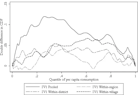
All our estimates are better seen as local average treatment effects (LATE), in the terminology of Angrist and Imbens (1995). The latter show that two-stage least squares instrumental variable estimations mechanically overweight the causal effect for those subgroups (here, income quantiles) that are the most affected by the instrument (here, by the double difference between cocoa-producers and other farmers). As the impact of family income on children outcomes is not necessarily the same at each quantile of the income distribution, one may wonder whether various IV estimates capture the same local effect of income. From this standpoint, the difference between our IV estimates at each level of spatial disaggregation would not only stem from the presence of contextual effects but also from distinct weighing schemes across the income distribution. Figure 4 plots double-differences

(24)

in income cumulative distribution functions (CDFs) for the four different levels of spatial disaggregation. It indeed reveals that the four estimates do not manipulate the same parts of the income distribution. Of course they do not manipulate the same amount either: cocoa producers lose more when they are compared with the whole sample of other farmers than when they are compared only with their neighbors. This is why it is useful to compare each double difference in CDF with a ”uniform counterfactual”, which we simulated by applying the same average change in mean to the income distribution observed in the 1986-88 sample of cocoa and non-cocoa farmers. Figure 5 provides the comparisons between the actual double-difference and the uniform simple difference in CDFs. In the end, both Figure 4 and Figure 5 show that pooled IV tends to overweight the bottom of the farmers income distribution whereas the within-villages IV places more weight at the top. Then, if only for school enrollment and child labor, part of the explanation for the differences between the four IV estimates presented in Table 6 could stem from the combination of two basic features: (i) they are local average treatment effects that do not manipulate the same parts of the income distribution; (ii) income elasticities school enrollment and/or child labor are higher (in absolute value) in the lower part of the distribution (among the poor) than in the upper part.8 _{Whereas the bias linked to contextual effects should lead us to prefer the}

highest level of spatial disaggregation (the village level), the local character of each estimate would lead us to value each of them equitably for not estimating the same weighted average of income elasticities. Of course, it is impossible for us

8_{One question is then why the manipulation of fixed effects allows us to exhibit those} het-erogeneous effects. A plausible explanation would be that the introduction of disaggregate fixed effects would select poor non-cocoa farmers that would have been relatively more affected by the loss of income of their cocoa neighbors and additionally affected by low prices and / or yields for their own culture (coffee producers in particular). Conversely, disregarding local effects gives more weight to the comparison of the poor cocoa farmers with poor non-cocoa farmers that were little affected over the period (especially cotton farmers in the more northern regions and staple producers close to urban areas).

(25)

to discriminate between the two potential explanations we have just given for the observed heterogeneity of the family income effect; as they are not incompatible, they may also share responsibility.

9 Conclusion

We study the drastic cut of the administered cocoa producer price in 1990 Cote d’Ivoire and look at the extent to which cocoa producers’ children suffered from this severe income shock in terms of school enrollment, increased labor, height stature and sickness. Comparing pre-crisis (1986-88) data and post-crisis (1993) data, we propose a difference-in-difference within-village strategy in order to iden-tify the causal effect of family income on children outcomes, whereby we compare the evolution of outcomes of children living in cocoa producing households with that of children living in other agricultural households of the same village. A sec-ond identification strategy exploits the weight of cocoa production in the district of birth of the children. With both strategies, we find a strong and significant impact of family income for the four variables we examine.

In comparison with the previous literature, we believe that our analysis of-fers several advantages. First, we exploit a negative income shock, for which no randomized experimental data will ever exist. Second, we not only examine child schooling and child labor, but also child care and child health, which are under-represented issues in the literature, especially in African countries. Third, using good microeconomic data on income, we are able to derive direct estimates of the causal effect of family income on children education and health. Fourth, we show that instrumenting with aggregate shocks may underestimate or overestimate the individual income effect, since contextual effects are not accounted for, hence our preference for the within-village strategy. Fifth, we indeed confirm that naive OLS estimation tends to underestimate the effect of household income. Sixth, our anal-ysis of local average treatment effects exhibits the possible heterogeneity of income effects along the income distribution.

(26)

African economies remain little diversified and vulnerable to changing in-ternational prices for their exports. In Cote d’Ivoire, a considerable part of the population still works in the agricultural sector, and directly undergoes the fluctu-ations of international prices. By the past, the national marketing board and price stabilization fund for cocoa and coffee, the Caisstab, did not really served its orig-inal mission; it was dismantled in 1998. Nevertheless, new insurance schemes and safety nets could be invented to protect households and children from unexpected shocks on income. If one believes in the income elasticities presented in this study, the transposition of conditional transfer programs already implemented in Latin America could deserve some attention, and could constitute a very defendable use of foreign aid money.

(27)

Figure 1: National Cocoa Producer Prices and Average Per Capita Consumption for Cocoa Producers and Non-Cocoa Farmers (Base 100 = Per Capita Consumption for Cocoa Households in 1988).

Sources: Berth´elemy and Bourguignon 1996, World Bank 2001, IMF 2007. Authors’ calculations.

Figure 2: Kernel Density of the Share of Cocoa Producers Within Villages where this Share is Positive.

(28)

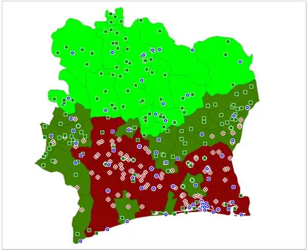
Figure 3: Average Cocoa Production by District in 1987-1988-1989 and Occupational Specialization of Surveyed Villages in 1986-1988 and 1993.

Reading: Light Grey Areas = no cocoa production, Dark Grey Areas = low density of cocoa production, Black Areas = high density of cocoa production. Production expressed in thousands of tonnes of cocoa beans per squared kilometer. Sources: CSSPPA (1990), DCGTx (1995). Authors’ calculations. Lozenges = cocoa producers are the most numerous group in the village, Squares = non-cocoa farmers are, Circles = non-agricultural households are.

(29)

Figure 4: Difference-in-Difference in Income CDFs for 5-11 y.o. Children.

Figure 5: Actual and Simulated (Uniform Shock) Difference-in-Difference in In-come CDFs for 5-11 y.o. Children (NW: pooled, NE: region, SW: within-district, SE: within-village).

(30)

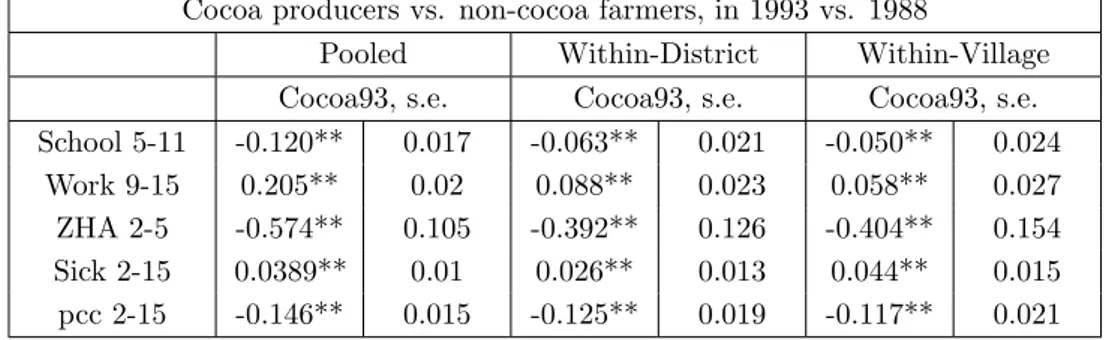
Table 1: Results for the Reduced-Form Model, School Enrollment (School 5-11), Child Labor (Work 9-15), Height-for-Age Z-score (HAZ 2-5) and Health Status (Sick 2-15).

Cocoa producers vs. non-cocoa farmers, in 1993 vs. 1988

Pooled Within-District Within-Village Cocoa93, s.e. Cocoa93, s.e. Cocoa93, s.e. School 5-11 -0.120** 0.017 -0.063** 0.021 -0.050** 0.024

Work 9-15 0.205** 0.02 0.088** 0.023 0.058** 0.027 ZHA 2-5 -0.574** 0.105 -0.392** 0.126 -0.404** 0.154 Sick 2-15 0.0389** 0.01 0.026** 0.013 0.044** 0.015 pcc 2-15 -0.146** 0.015 -0.125** 0.019 -0.117** 0.021

Regressions: OLS, pooled or within-district/village (including time-district or time-village fixed effects), robust to heteroscedasticity, including N agri, N agri1993, dummies for age, gender and cocoa specialization and their multiple interactions as well as time dummies for pooled regressions. pcc: log of per capita consumption. Obs. 5-11: 20657, 9-15: 17829, 2-5: 8764, 2-15: 39123. ** significant at 5%, * significant at 10 %.

(31)

Table 2: Mean Characteristics for 2-15 y.o. Children for Cocoa Producers and Non-Cocoa Farmers, in 1988.

Non-Cocoa Cocoa

Age 7.915 8.113**

Sex 0.534 0.551*

Was born out of Ivory Coast 0.007 0.008 Was not born in the district of residence 0.140 0.109** Is the biological child of HH head 0.698 0.744** Size of the HH 10.08 10.9** Age of HH head 50.24 50.77** HH head is a woman 0.079 0.026** HH head has ever been to school 0.175 0.267** HH head has at least achieved prim. school 0.112 0.159** HH owns livestock 0.654 0.608** HH head has migrated in the last 3 years. 0.065 0.041** HH head was born out of Ivory Coast 0.071 0.137**

Obs. 2-15: 39123. Stars indicate whether means between cocoa producers and other farmers are stastically significant. ** significant at 5%, * significant at 10%.

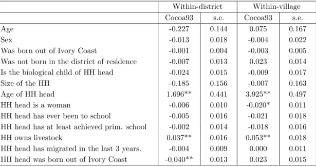
Table 3: Relative 1988-1993 Change in Observables for 2-15 y.o. Children between Cocoa Producers and Non-Cocoa Farmers.

Within-district Within-village Cocoa93 s.e. Cocoa93 s.e. Age -0.227 0.144 0.075 0.167 Sex -0.013 0.018 -0.004 0.022 Was born out of Ivory Coast -0.001 0.004 -0.003 0.005 Was not born in the district of residence -0.007 0.013 0.023 0.014 Is the biological child of HH head -0.024 0.015 -0.009 0.017 Size of the HH -0.185 0.156 -0.007 0.163 Age of HH head 1.696** 0.441 3.925** 0.497 HH head is a woman -0.006 0.010 -0.020* 0.011 HH head has ever been to school -0.005 0.016 -0.021 0.018 HH head has at least achieved prim. school -0.002 0.014 -0.018 0.016 HH owns livestock 0.037** 0.016 0.053** 0.018 HH head has migrated in the last 3 years. -0.004 0.009 0.000 0.011 HH head was born out of Ivory Coast -0.040** 0.013 0.023 0.015

Regressions: OLS-within-district/village (including time-district or time-village fixed effects), robust to het-eroscedasticity. Obs. 2-15: 39123. ** significant at 5%, * significant at 10 %.

(32)

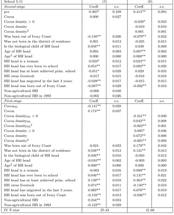
Table 4: IV1 and IV2 Second-Stage and First-Stage Results for School Enrollment, 5-11 y.o. Children.

School 5-11 (5) (6)

Second-stage Coeff. s.e. Coeff. s.e.

pcc 0.305* 0.169 0.414** 0.094

Cocoa 0.000 0.027

Cocoa density > 0 -0.039* 0.023

Cocoa density -0.010 0.010

Cocoa density2 _0.001 _0.001

Was born out of Ivory Coast -0.150** 0.026 -0.079** 0.032 Was not born in the district of residence 0.001 0.013 -0.025 0.015 Is the biological child of HH head 0.058** 0.011 0.039 0.009 Age of HH head 0.004 0.003 0.007** 0.002 Age2 _{of HH head} _0.000 _0.000 _0.000** _0.000 HH head is a woman 0.023* 0.012 0.024** 0.015 HH head has ever been to school 0.054** 0.017 0.082** 0.020 HH head has at least achieved prim. school 0.051* 0.028 0.029 0.033 HH owns livestock -0.017 0.015 -0.016 0.016 HH head has migrated in the last 3 years. -0.039** 0.017 -0.015 0.015 HH head was born out of Ivory Coast -0.087** 0.029 -0.092** 0.010 Non-agricultural HH -0.006 0.040

Non-agricultural HH in 1993 -0.002 0.026

First-stage Coeff. s.e. Coeff. s.e.

Cocoa93 -0.141** 0.028 Cocoa 0.174** 0.037 Cocoa density93> 0 -0.241** 0.030 Cocoa density93 0.042** 0.008 Cocoa density932 _-0.002** _0.001 Cocoa density > 0 0.085* 0.046 Cocoa density 0.072** 0.006 Cocoa density2 _-0.005** _0.000

Was born out of Ivory Coast 0.024 0.033 0.179** 0.042 Was not born in the district of residence 0.048** 0.012 0.121** 0.013 Is the biological child of HH head 0.038** 0.010 -0.003 0.012 Age of HH head -0.010** 0.002 -0.003 0.003 Age2 _{of HH head} _0.000** _0.000 _0.000 _0.000 HH head is a woman -0.003 0.016 0.080** 0.019 HH head has ever been to school 0.046** 0.017 0.131** 0.021 HH head has at least achieved prim. school 0.139** 0.018 0.304** 0.022 HH owns livestock 0.074** 0.011 -0.150** 0.010 HH head has migrated in the last 3 years. 0.069** 0.017 0.070** 0.019 HH head was born out of Ivory Coast -0.158** 0.013 -0.036** 0.012 Non-agricultural HH 0.244** 0.024

Non-agricultural HH in 1993 -0.122** 0.029

IV F-stat 25.43 21.66

Columns: (5) IV1-within-village, (6) IV2 with cocoa density > 0, cocoa density and cocoa density squared. Non-reported controls: dummies for age, gender and cocoa specialization and their multiple interactions, and time dummies for IV2 regressions. pcc: log of per capita consumption. Obs. 5-11: 20657. ** significant at 5%, * significant at 10 %.

(33)

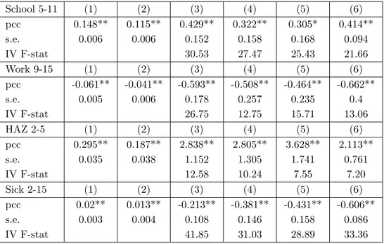
Table 5: Results for School Enrollment (School 5-11), Child Labor (Work 9-15), Height-for-Age Z-score (HAZ 2-5), and Health Status (Sick 2-15).

School 5-11 (1) (2) (3) (4) (5) (6) pcc 0.148** 0.115** 0.429** 0.322** 0.305* 0.414** s.e. 0.006 0.006 0.152 0.158 0.168 0.094 IV F-stat 30.53 27.47 25.43 21.66 Work 9-15 (1) (2) (3) (4) (5) (6) pcc -0.061** -0.041** -0.593** -0.508** -0.464** -0.662** s.e. 0.005 0.006 0.178 0.257 0.235 0.4 IV F-stat 26.75 12.75 15.71 13.06 HAZ 2-5 (1) (2) (3) (4) (5) (6) pcc 0.295** 0.187** 2.838** 2.805** 3.628** 2.113** s.e. 0.035 0.038 1.152 1.305 1.741 0.761 IV F-stat 12.58 10.24 7.55 7.20 Sick 2-15 (1) (2) (3) (4) (5) (6) pcc 0.02** 0.013** -0.213** -0.381** -0.431** -0.606** s.e. 0.003 0.004 0.108 0.146 0.158 0.086 IV F-stat 41.85 31.03 28.89 33.36

Columns: (1) OLS-within-district, (2) OLS-within-village, (3) IV1-within-district, (4) IV1-within-village; (1) to (4) models include dummies for age, gender and cocoa specialization and their multiple interactions (in the case of height-for-age Z-score, only dummies for cocoa specialization and the interactions between age in months and gender) plus N agri and N agri1993; (5) IV1-within-village with additional controls (list provided below); (6) IV2 with cocoa density > 0, cocoa density and cocoa density squared. First set of additional controls: age and age squared of the household head, dummies variables for the child was not born in Ivory Coast, for the household head was not born in Ivory Coast, is a woman, has ever been to school, has achieved at least primary schooling, and for the household owns livestock. Second set of additional controls (regression not shown): is the youngest child, is the youngest boy, was not born in the region of residence, household owns a business, number of household head spouses, head or spouse is a civil servant, head has migrated in the last year, head’s main ethnical group and main religion, number of rooms in the accommodation, access to water, access to electricity, household owns a bicycle, household owns a radio. pcc: log of per capita consumption. Obs. 5-11: 20657, 9-15: 17829, 2-5: 8764, 2-15: 39123. ** significant at 5%, * significant at 10 %.

(34)

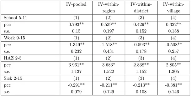
Table 6: IV1 Results for School Enrollment (School 5-11), Child Labor (Work 9-15), Height-for-Age Z-score (HAZ 2-5) and Health Status (Sick 2-15) according to the Spatial Disaggregation of Fixed Effects.

IV-pooled IV-within-region IV-within-district IV-within-village School 5-11 (1) (2) (3) (4) pcc 0.793** 0.539** 0.429** 0.322** s.e. 0.15 0.197 0.152 0.158 Work 9-15 (1) (2) (3) (4) pcc -1.349** -1.518** -0.593** -0.508** s.e. 0.232 0.431 0.178 0.257 HAZ 2-5 (1) (2) (3) (4) pcc 3.961** 3.683* 2.838** 2.805** s.e. 1.137 1.522 1.152 1.305 Sick 2-15 (1) (2) (3) (4) pcc -0.291** -0.211** -0.213** -0.381** s.e. 0.079 0.129 0.108 0.146

Columns: (1) IV1, (2) IV1-within-region (including time-region fixed effects), (3) IV1-within-district (including time-district fixed effects), (4) IV1-within-village (including time-village fixed effects). (1) to (4) models include dummies for age, gender and cocoa specialization and their multiple interactions Obs. 5-11: 20657, 9-15: 17829, 2-5: 8764, 2-15: 39123. pcc: log of per capita consumption. ** significant at 5%, * significant at 10 %.

(35)

APPENDIX 1: Schooling and Health in Cote d’Ivoire: Facts

Cote d’Ivoire, like its neighboring Western African countries, is a demographically young country to the extent that the share of children aged 0 to 14 is high in the total population: 46.1% (UN 2007). The Ivorian educational system proposes the following curriculum: from 5 to 11, ”école primaire”, from 12 to 15, ”collège”, from 16 to 18, ”lycée” (high school), and from 19, ”université”. Actually, children enter rather late into the first grade of primary schooling (”Cours Préparatoire 1ère année”, CP1). In our specific sample, the average entry age into primary schooling is 7.33 (and not 5 as in theory). Girls seem to enter slightly sooner than boys (6.93 vs 7.61 for the latter). Then, less than half of children attend primary schooling, and even less achieve the full cycle. In our 1988 sample, amongst the children aged 9 to 15, 50% only attend school, 3.6% both attend school and work, and 25.4% only work. As for nutritional and mortality indicators, Cote d’Ivoire performs rather well in comparison with other West African countries, even if this country is the West African country where the AIDS epidemics is the most widespread.

Table 7: Investments in Education and Health for Five West African Countries

Burkina-Faso

Cote d’Ivoire

Ghana Guinea Mali Net primary education enrolment ratio, 1990

(%)

26.2 45.6 52.4 25.5 20.4 Completion rate of primary schooling, 1991

(%)

21.3 43.4 62.8 16.8 10.8 Completion rate of primary schooling, girls

only, 1991 (%)

16.1 32.2 54.9 9.1 8.5 Percentage of pupils starting grade 1 and

reaching grade 5, 1991

69.7 72.5 80.5 58.6 69.7 % of children under 5 who are stunted 43.1

(2003) 31.5 (1999) 35.6 (2003) 39.3 (2005) 42.7 (2001) % of children under 5 who are underweight 35.2

(2003) 18.2 (1999) 18.8 (2003) 22.5 (2005) 30.1 (2001) % of newborns with low birth weight, 2002 19 17 11 12 23 Under-5 mortality rate (per 1000 live births),

1990

210 157 122 240 250

Children under 5 years of age with diarrhoea who received oral rehydratation therapy (%)

62.8 (2004) 66.1 (2000) 63.3 (2004) 56.7 (2005) 65.7 (2002) Children under 5 years of age with acute

respiratory infection and fever taken to facility (%) 32.6 (2004) 34.9 (2000) 44 (2004) 34.5 (2005) 42.8 (2002) Sources: UN, 2007 and WHO, 2007

(36)

References

[1] Angrist, J. and G. Imbens (1995). ”Two-Stage Least Squares Estimation of Average Causal Effects in Models with Variable Treatment Intensity”, Journal of the American Statistical Association, Vol. 90, No. 430, 431-442.

[2] Azam, J.-P. (1993). ”The Cote d’Ivoire Model of Endogenous Growth”, Eu-ropean Economic Review, 37:2-3, 566-576.

[3] Banerjee A., E. Duflo, G. Postel-Vinay, and T. Watts (2007). ”Long Run Health Impacts of Income Shocks: Wine and Phylloxera in 19th Century France”, NBER Working Paper, No. 12895.

[4] Beegle K., R. Dehejia and R. Gatti (2006). ”Child Labor and Agricultural Shocks”, Journal of Development Economics, 81(1): 80-96.

[5] Behrman J. and J. Knowles (1999). ”Household Income and Child Schooling in Vietnam”, World Bank Economic Review, 13(2): 211-56.

[6] Berth´elemy J.-C. and F. Bourguignon (1996). ”Growth and Crisis in Cote d’Ivoire”, World Bank.

[7] Bertrand M., E. Duflo, and S. Mullainathan (2004), ”How Much Should We Trust Differences-in-Differences Estimates?”, The Quarterly Journal of Eco-nomics, 119(1):249-275.

[8] Blau, D.M. (1999). ”The Effect of Income on Child Development”, Review of Economics and Statistics, 81(2):261-277.

[9] Bommier, A. and S. Lambert (2000). ”Education Demand and Age at School Enrollment in Tanzania”, Journal of Human Resources, 35(1):177-203.

[10] Cameron, S.V and J.J. Heckman (1998). ”Life Cycle Schooling Decisions, and Dynamic Selection Bias: Models and Evidence for Five Cohorts of American Males”, Journal of Political Economy, 106(2): 262-334.

(37)

[11] Case, A. (2001). ”Does Money Protect Health Status? Evidence from South African Pensions”, NBER Working Paper, No. 8495.

[12] Cogneau, D. and S. Mespl´e-Somps (2003). ”Les illusions perdues de l’´economie ivoirienne et la crise politique”, Afrique Contemporaine, 206: 87-104.

[13] CSSPPA (1990), ”Statistiques de production de cacao”, R´epublique de Cote d’Ivoire.

[14] DCGTx (1995), ”Cote d’Ivoire, Statistiques macro-´economiques”, R´epublique de Cote d’Ivoire, 25 p.

[15] Deaton, A. (1997). The Analysis of Household Surveys: A Microeconomet-ric Approach to Development Policy, Washington: Johns Hopkins University Press, World Bank.

[16] Deaton, A. (2007). Height, Health and Development, Proceedings of the Na-tional Academy of Sciences, 104(33): 13232-13237.

[17] Deaton, A. and J. Dreze (2008). ”Nutrition in India: Facts and Interpreta-tions”, mimeo.

[18] De Janvry A., F. Finan, E. Sadoulet and R. Vakis (2006). ”Can Conditional Cash Transfers Serve as Safety Nets to Keep Children at School and Out of the Labor Market?”, Journal of Development Economics, 79(2):349-373.

[19] Duflo, E. (2000). ”Child Health and Household Resources in South Africa: Evidence from the Old Age Pension Program”, American Economic Review, 90(2): 393-398.

[20] Duflo, E. (2003). ”Grandmothers and Granddaughters: Old-Age Pensions and Intrahousehold Allocation in South Africa”, World Bank Economic Review, 17: 1-25.

(38)

[21] Edmonds, E. and N. Pavcnik (2005). ”The Effect of Trade Liberalization on Child Labor”, Journal of International Economics, 65(2): 401-419.

[22] Edmonds, E. (2006). ”Child Labor and Schooling Responses to Anticipated Income in South Africa”, Journal of Development Economics, 81(2): 386-414.

[23] IMF (2007). International Monetary Fund, World Economic Outlook Databases.

[24] Grimm M. (2004). ”A Decomposition of Inequality and Poverty Changes in the Context of Macroeconomic Adjustment : A Microsimulation Study for Cote d’Ivoire”, in Shorrocks A. F. and R. van der Hoeven (eds), Growth, Inequality and Poverty. Prospects for Pro-Poor Development, Oxford: Oxford University Press.

[25] Hausman J., J.H. Stock and M. Yogo (2005). ”Asymptotic Properties of the Hahn-Hausman Test for Weak-Instruments,” Economics Letters, 89(3): 333-342.

[26] Jensen, R. (2000). ”Agricultural Volatility and Investments in Children”, American Economic Review, 90(2): 399-404.

[27] Jones, C. and X. Ye (1997). ”Issues in Comparing Poverty Trends over Time in Cote d’Ivoire”, World Bank Policy Research Working Paper, 1711.

[28] Kruger, D. (2007). ”Coffee Production Effects on Child Labor and Schooling in Rural Brazil”, Journal of Development Economics 82: 448-463.

[29] Maddison, A. (2003). The World Economy: Historical Statistics, Development Centre Studies, Paris: OECD.

[30] Martorell, R. and J. Halbicht (1986). ”Growth in Early Childhood in Devel-oping Countries”. In ”Human Growth: A Comprehensive Treatise”, ed. F. Falkner and J.M. Tanner, 2nd ed., vol. 3, NY: Plenum Press.

(39)

[31] Moradi, A. (2006). ”Nutritional Status and Economic Development in sub-Saharan Africa 1950-1980”, GPRG Working Paper, No 046.

[32] Schaffer, M. (2007). ”Xtivreg2: Stata Module to Perform Extended IV/2SLS, GMM and AC/HAC, LIML and k-class Regression for Panel Data Models”.

[33] Schultz, T. P. (2004). ”School Subsidies for the Poor: Evaluating the Mexican Progresa Poverty Program”, Journal of Development, Economics, 74(1): 199-250.

[34] Thomas D., K. Beegle, E. Frankenberg, B. Sikoki, J. Strauss and G. Teruel (2004). ”Education in a Crisis”, Journal of Development Economics, 74(1): 53-85.

[35] UN (2007). United Nations, Common Database (UNDCB).

[36] WHO Multicentre Growth Reference Study Group (2006). WHO Child Growth Standards: Length/height-for-age, weight-for-age, weight-for-length, weight-for-height and body mass index-for-age: Methods and development. Geneva: World Health Organization.

[37] WHS (2007). World Health Statistics 2007, WHO Statistical Information Sys-tem.