The correlation of electrochemical and magnetic techniques for use in characterization of underfilm corrosion

The Correlation of Electrochemical and Magnetic

Techniques for use in Characterization of

Underfilm Corrosion

by

Suzanne L. Wallace

B.S., Johns Hopkins University (1997)

Submitted to the Department of Materials Science and Engineering

in partial fulfillment of the requirements for the degree of

Master of Science in Materials Science and Engineering

at the

MASSACHUSETTS INSTITUTE OF TECHNOLOGY

June 1999

©

Massachusetts Institute of Technology 1999. All rights reserved.

A uthor .. . ... ...

'9

Department of Materials Science and Engineering

May 07, 1999

Certified by.... ...

-. ...

r. ...

Professor Ronald M. Latanision

Director, H. H. Uhlig Corrosion Lab

Thesis Supervisor

A ccepted by ...

...

Linn W. Hobbs, John F. Elliott Professor of Materials

Chairman, Departmental Committee on Graduate Students

MASSACHUSETTS INSTITUTE

OF TECHNOL

The Correlation of Electrochemical and Magnetic

Techniques for use in Characterization of Underfilm

Corrosion

by

Suzanne L. Wallace

Submitted to the Department of Materials Science and Engineering on May 07, 1999, in partial fulfillment of the

requirements for the degree of

Master of Science in Materials Science and Engineering

Abstract

Coated systems are used in many different applications. These systems, while less susceptible to corrosion than uncoated systems, are not impervious to corrosion. Since there is a coating, however, the traditional corrosion measurement techniques can not be used. Techniques such as electrochemical impedance spectroscopy (EIS) have been applied in this capacity. While EIS is useful in monitoring the degradation of the system, it has not previously been possible to definitively show a correlation between corrosion rate and mass loss data.

To quantify the mass loss and corrosion rate, an established technique from an-other discipline was used. The vibrating sample magnetometer (VSM) records the magnetic moment of a sample and the corresponding applied field. The magnetic saturation of a ferromagnetic material is a structure insensitive material property; thus it only changes with a change in mass and/or volume of a material. When a material is corroded it loses mass, and this mass change is detectable with a VSM.

The goal is to use the magnetic technique in conjunction with the electrochem-ical technique to determine mass loss and corrosion rate for a coated system. The groundwork for this was laid here. First the mass loss determined from gravimet-ric, electrochemical, and magnetic methods was correlated. This indicates that the methodology is possible. Next, the comparison between VSM and EIS data is neces-sary.

Before coated samples were used, bare cobalt foils and silicon wafers with sputter deposited cobalt were tested. The results of electrochemical and magnetic testing re-vealed a 1:1 relationship between the percent change in mass and the percent change in magnetic saturation. Samples were then coated with either an acrylic or a poly-imide and were then tested using electrochemical impedance spectroscopy.

Thesis Supervisor: Professor Ronald M. Latanision Title: Director, H. H. Uhlig Corrosion Lab

Acknowledgments

This research was supported by an NSF grant for the study of the fundamental aspects of underfilm corrosion. It was an international collaboration of some great people from three different countries. My gratitude is owed to these people: Prof. Ron Latanision and Dr. Bryce Mitton of MIT, Prof. George Thompson of UMIST in England, and Prof. Francesco Bellucci and Mr. Luca DeRosa of the University of Naples in Italy.

I would not have made it around the lab without the help of the wonderful group

of people assembled in the H.H. Uhlig Corrosion Lab. First I owe my advisor, Prof. Latanision, for the opportunity to take part in this project. Bryce knows how much I owe him for everything. Dr. Gary Leisk and soon-to-be-Dr. Jason Cline were the best and most helpful office mates I could have had. Dr. Geetha Berera, Dr. Jae-Hong Yoon, Dr. Young-Sik Kim, and Dr. Seisho Take were always there to support me. Ellie Bonsaint made the administrative side of things easier. Although we started working together late in this project, Amy Lin was a great UROP. And I am grateful that what was started here will be continued by Nicolas Cantini, and of course, Bryce. This thesis would never have been completed without the support and force of some helpful guys. I am quite glad that Sean George and Jason convinced me that LTEXwas the way to go when writing my thesis, it was much smoother than I antic-ipated. Whenever I had questions while working on Athena, Alex Budge was always there to patiently answer them. I can not imagine how to express my gratitude to Sean and Gary for their assistance with assembling my thesis seminar transparencies. As always, I must thank the people who supported my decision to pursue a grad-uate degree, and all of my decisions; my parents John and Linda Wallace, and my sister, Shannon. And finally, thanks to Sean for being there over these past two years when I've fallen apart and when I've succeeded.

Contents

2.5.2 _{Electrochemical Impedance Spectroscopy . . . . 24}

2.6 _{Experimental Setup . . . . 29}

2.6.1 _{Samples . . . . 29}

2.6.2 _{Electrochemical Cell . . . . 32}

2.6.3 _{Equipment . . . . 33}

2.7 Results and Discussion . . . . 34

2.7.1 _{Potentiodynamic and Potentiostatic Scans . . . . 34}

2.7.2 _{Linear Polarization . . . . 42}

2.7.3 _{Electrochemical Impedance Spectroscopy . . . . 45} 3 Magnetics

3.1 _{Ferromagnetism . . . .} 52

3.2 Properties and Hysteresis Loop . . . .

3.3 Cobalt . . . . 3.4 Measurement Instrumentation . . . . 3.4.1 Vibrating Sample Magnetometer . . .

3.4.2 Magnetics and Corrosion . . . .

3.5 Experimental Setup . . . .

3.5.1 Sam ples . . . .

3.5.2 Equipment . . . .

3.6 R esults . . . .

4 Correlation of Electrochemical and Magnetic

4.1 Combination of Data from All Techniques . .

4.2 Error... ... 5 Conclusions and Future Work

A List of Symbols B List of Abbreviations Techniques 53 55 57 57 59 60 60 60 62 67 67 70 72 76 78

List of Figures

2-1 Schematic Cross Section of Underfilm Corrosion . . . . 15

2-2 Potential-pH Diagram for Cobalt . . . . 19

2-3 Potentiostat Controlled Measurement Setup . . . . 22

2-4 Impedance Relationships . . . . 25

2-5 _{RC Circuits and Corresponding Impedance Spectra . . . . 26}

2-6 _{Equivalent Circuit and Corresponding Bode Plots for Coated System 28} 2-7 SEM Cross Section of PI-Coated Cobalt-Silicon Wafer . . . . 31

2-8 EIS Test Cell . . . . 33

2-9 Polarization Curves in 0.5 M NaCl for Foil and Wafer Cobalt Samples 35 2-10 Polarization Curves for Cobalt Foil Samples in Both Solutions . . . . 36

2-11 Potentiostatic Scan Performed at -170 mV vs. SCE . . . . 38

2-12 Uniform Corrosion in Acidified Solution . . . . 39

2-13 Pitting Corrosion in 0.5 M NaCl . . . . 40

2-14 Comparison of Electrochemical and Gravimetric Mass Loss Data . . . 41

2-15 Linear Polarization Curves Generated at Different Times . . . . 42

2-16 Comparison Between Experimental and Theoretical Plots . . . . 44

2-17 Corrosion Current With Time . . . . 45

2-18 Bare Cobalt Foil Impedance Spectra . . . . 46

2-19 Initial High Impedance of the Acrylic Coating . . . . 47

2-20 Underfilm Corrosion Initiating in Surface Defects . . . . 48

2-21 Underfilm Corrosion, Close-up . . . . 49

2-22 Coated Cobalt Foil Impedance Spectra . . . . 50

3-1 Magnetic Hysteresis Loop . . . . 54

3-2 Diagram of VSM . . . . 58

3-3 DMS Model 880 VSM . . . . 61

3-4 Comparison of Cobalt Foil and Wafer Hysteresis Loops . . . . 63

3-5 Decrease in Saturation After Corrosion . . . . 64

3-6 Comparison of Saturation Change and Gravimetric Mass Loss Data . 65 4-1 Comparison of Magnetic Saturation Change and Electrochemical Mass Loss ... ... 68

List of Tables

2.1 _{Electrochemical Data . . . . 34}

3.1 _{Magnetic Properties of Cobalt . . . . 56}

Chapter 1

Introduction

Corrosion is a problem that has always affected mankind, and while it can currently be controlled to some extent, it will likely always exist. Each year it costs the US about $30 billion [1] in maintenance, repairs, and lost production time. A large part of that cost could be saved by utilizing the methods of protection and prevention available.

The protection and prevention methods available today consist of three main cat-egories: materials selection and design, cathodic and anodic protection, and coatings

[1]. Materials selection and design is the easiest to employ, since it should be a

fun-damental part of any engineering project. Cathodic and anodic protection involve either actively polarizing a system or employing a sacrificial system in connection with the main one. The third, coatings, finds widespread use in many different in-dustries, such as microelectronics, automotive, infrastructure and construction, and food packaging. The primary function of these coatings is to act as a physical and chemical barrier between the corrosive environment and the structure being protected [2]. These coatings are not permanent solutions to corrosion issues, however. With time they can degrade through mechanical or chemical attack, and when the coat-ing is compromised, corrosion begins to occur at the coatcoat-ing/metal interface. This corrosion beneath the coating is termed underfilm corrosion.

While it is known that underfilm corrosion takes place, and it can currently be detected visually after it has begun, and monitored electrochemically; there is much

yet to be learned on this subject. One problem of coated systems is delamination of the polymer. It is not known whether this delamination is due to a simple loss of adhesion or due to corrosion reactions and products at the interface. Methods are available to detect the existence of corrosion as well as the existence of delamination; however, currently there is not an exact technique to determine if the delamination was due to loss of adhesion from the swelling polymer and water aggregation or due to the corrosion occuring at the interface.

Techniques such as Electrochemical Impedance Spectroscopy (EIS) monitor the underfilm corrosion [3], but EIS can do no more than estimate the corrosion rate. Traditional corrosion testing methods which yield corrosion rates, involve knowledge of the mass loss of the material. Most simply, this can be done by weighing the sample before and after corrosion. A problem with coated systems is that an accurate mass loss measurement is difficult to make. The coating can swell when introduced to an electrolyte and it can trap corrosion products, causing inaccurate mass measurements. For non-coated, or bare metal samples, the relationship between the electrochemical data and the mass loss is well established in the literature [4] [2]. But for coated systems, this has not yet been satisfactorily achieved.

To establish a relationship between electrochemistry and mass loss of a coated system, a different approach to measuring mass loss had to be found. Certain metals known as ferromagnets exhibit a material property called magnetic saturation, (MS). Saturation can be measured as an absolute value that is a known quantity when normalized by sample mass and volume [5]. Thus saturation is affected only by the amount of magnetic material. The change in the relative saturation can be used to indicate change in mass and volume of the metal [6]. It is possible to use a change in saturation to determine the corrosion rate by correlating the change in saturation and mass loss. The saturation measurements are not significantly affected by the polymer nor by non-ferromagnetic oxides present as corrosion products. Another potential benefit of employing magnetic measurements is that it should be possible to differentiate between delamination due to loss of adhesion or corrosion. Thus, only delamination due to corrosion can be detected by magnetic testing because only in

this case will there be a loss of magnetic material.

The study performed here used magnetic methods to correlate mass loss and electrochemical data for both a polymer coated metal and a non-coated metal. The next chapter will briefly explain the background of the corrosion principles employed here as well as the experimental setup and results of the electrochemical testing. Chapter 3 will do the same for the magnetics aspect of the project. The ensuing chapters will correlate the corrosion and magnetics results, the ultimate goal of this work.

Chapter 2

Corrosion

2.1

Background

Corrosion is a chemical reaction that occurs between a material and its environment. This is usually considered a destructive reaction that results in a loss of the material. Metallic corrosion involves charge transfer as the result of an oxidation reaction and a reduction reaction. The common anodic reaction is

M <4 Mn+ + ne~

The corresponding cathodic reaction in an aqueous media is frequently one of the following:

2H+ + 2e- <+ H2(g)

02 + 2H20+ 4e +

40H-Water dissociation, which is essentially equivalent to the hydrogen reduction reaction, can also occur

2H20 + 2e- 4 H2(g) +

20H-Determination of the reaction kinetics is important, it yields information about corrosion rates. The rate of electron charge transfer gives a good measure of the

reaction rates of corrosion. The current density, defined as the current (electron flow) per surface area, is proportional to the corrosion rate. Along with a current, there is a corresponding potential in the electrochemical cell which is a corroding metal.

A steady state potential known as the corrosion potential, Ecorr, defines where

the system is in an equilibrium with respect to the exchange of electrons due to the anodic and cathodic reactions. As the system's potential fluctuates from Ecorr the potential change is referred to as polarization, or over-potential.

Another useful tool in studying corrosion is a quantity known as the Tafel constant. This constant relates polarization and current density. This is represented by the equation

io

S= s log -(2.1)

where q is the polarization, 3 is the Tafel constant, and i is the current density. The

Tafel constant is usually in units of volts per decade. When the potential is plotted as a function of the log of the current density, the Tafel region, where this relationship holds, is a linear portion of the curve near the corrosion potential. This Tafel zone exists for both the cathodic and anodic reactions, and, in addition there are different corresponding constants for the two reactions.

2.2

Underfilm Corrosion

In a coated system, the degradation of the coated metal is governed by the same general corrosion reactions stated above, the difference is the protection provided by the coating. Thus, the entire corrosion process is not governed only by the electrolyte solution and the metal interactions, but also by the behavior of the organic coating.

For a polymer system to provide long-term protection, it must demonstrate strong mechanical resistance and adhesion, chemical stability, and low permeability [7]. The mechanical resistance and adhesion reflect the strength of the bond between the coating and the metal substrate. The coated system might be subjected to various loads in the working environment, and the coating should be able to withstand them. Chemical stability refers to the ability of the coating to maintain integrity during

chemical attack from such things as water, radiation, temperature, and different salts and ions. Permeability reflects the water or solution uptake of the coating. The lower the permeability of the coating to moisture, the lower is the probability that the substrate will encounter that environment.

There are two main mechanisms involved in protection by coatings, barrier be-havior and reactions due to additives in the coating [8] [9]. As a barrier, the coat-ing limits diffusion of water, oxygen, ionic species, and other corrosive agents. No coating is ever impermeable to these compounds, but the amount a coating limits permeation is a function of its capability to protect the substrate [10]. In resisting transport through the coating, it is also necessary to resist the transport laterally along the metal/coating interface. The additives in a coating can passivate the metal substrate, behave as an inhibitor to corrosion, or provide cathodic protection.

A coating will not function as a very good barrier if it is compromised. Thus the

application of the film is often the limiting step in the performance of a coating [11].

A poor application can result in defects such as uneven regions, pinholes, cracks or

crazes, local uncured zones, and nonuniform cross-linking. Since underfilm corrosion is usually a local event, even such small defects may initiate substrate degradation. A key factor in determining performance is the quality of the bond between the metal and the polymer. Often the bond is not with the metal itself, but with the native oxide film that has formed on the metal's surface [12]. The surface finish of the substrate is also quite relevant to the bond formed. Generally, smooth surfaces are considered to be superior since a polymer applied in the liquid form can achieve good contact. When the surface is rough, polymer penetration into the various topography depends on contact angle and pore shape of the surface, as well as the viscosity and flow properties of the polymer [13]. A good bond requires extensive molecular contact, which is affected by the surface energies and contact angles of the substrate and polymer. Organic polymers generally exhibit low contact angles on high energy substrates, but surface contaminations would lower these energies. Roughness does limit the contact with the polymer, but with a low contact angle and a low viscosity, an extended time before the cure or set can allow for a good bond [13]. One benefit

Na+ COATING

H2 NO M+

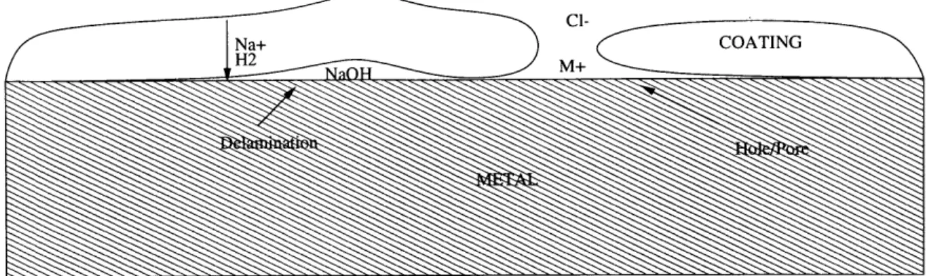
Figure 2-1: Schematic Cross Section of Underfilm Corrosion

of surface roughness is that it can alter the stress distribution of the surface, which can enhance bonds. Once a polymer is actually in use, however, the maintenance of a minimum level of adhesion is much more important than the initial bond strength [14].

Another common mode of coating failure is delamination [15] [8] [9]. This can occur due to a number of different processes. One can be poor wet adhesion, the aggregation of water at the polymer/metal interface weakens the adherence of the coating to the substrate. Another potential cause is cathodic delamination. The cathodic corrosion reaction, the oxygen reduction, creates a high pH environment which leads to delamination. The coating can also delaminate when the polymer swells due to uptake of the electrolyte solution. A schematic of delamination as a mode of underfilm corrosion can be seen in Figure 2-1. This shows a region of delamination occurring and a region where it has already occurred due to a defect such as a pore or hole or anything that allows the substrate and the solution to be in free contact and free ion exchange. In the region marked delamination there is an alkaline environment shown, the result of the cathodic corrosion reaction.

As in corrosion in the absence of a coating, corrosion underneath a polymer re-quires cathodic and anodic reactions. The reacting species need to migrate to the polymer/metal interface. This migration takes place through a few different methods. These pathways include activated diffusion, nonactivated diffusion, and interfacial

diffusion [8]. The nonactivated, or passive diffusion takes place through defects in a coating such as pores and pinholes. The uptake of water and ionic species is related to the diffusivity of the species in the organic medium, or the permeability of that medium. Migration of ions can also occur due to a gradient that is set up in the system, the coating/environment interface has one concentration of species or charge while the coating/metal interface has another, thus driving the electrolytes along the gradient. Interfacial diffusion occurs when there is already some water or solution aggregated at the metal/coating interface. The diffusion then occurs laterally along the interface. The migration of these ions may lead not only to corrosion but also to blistering of the coating and delamination [7]. This blistering is seen in regions where ionic conduction through the coating is enhanced.

2.3

Polymeric Coatings

Coatings can consist of many types of materials such as organic polymers, ceram-ics, or metallics [2]; however, polymers make up a majority of the coatings in use. Two specific coatings are of interest here. A polyimide coating is commonly used in microelectronics and an acrylic coating is used in the automotive industry.

2.3.1

Polyimides

Polyimides are formed through a two step process. The first step synthesizes polyamic acid from an aromatic diamine with pyromellitic dianhydride [16]. This is then applied to a substrate. The second step consists of heating the system between 200 and 400

'C to produce the polyimide. This process is an imidization reaction which releases

water as a by-product. During this process an interaction between the polyamic acid and the metal substrate, or surface oxide, may occur which leads to chemical bonding and results in good adhesion [17]. This reaction is substrate dependent, however, and in some cases an adhesion promoter must be used.

In the field of semiconductor devices these polymers are used in two main roles: protection and interlayer dielectrics. As a protective polymer, polyimides are

ap-plied as junction coatings, buffer coatings, a-ray shielding, and in passivation roles. The advantages to using polyimides in this field are many-heat and chemical resis-tance, low dielectric constant, low temperature processing, elasticity, and absorption of mechanical stress. The disadvantages are lower thermal stability than some other polymer options, and high moisture absorption and penetration [18].

Polyimides have frequently been the study of underfilm corrosion research [19] [20] as the area of microelectronics is particularly sensitive to this form of corrosion. The amount of metal used in semiconductor devices is so minute that once initiated, corrosion can quickly destroy it. An example of a problem region is in the inner layers of a multi-layered microelectronic structure. This structure is composed of many alternating layers of dielectrics and metals, often more than one type of metal. These layers corrode more quickly than the outer layers because of the increased number of interfaces with different materials. Utilizing polyimides in these devices has brought about a decrease in this problem [18].

2.3.2

Acrylics

The type of acrylic used during this research project is a thermoset resin. These resins react chemically after they are applied. They contain functional groups that can react with different functional polymers or cross-linkers. A common functional polymer is a melamine-formaldehyde (MF). The acrylic is prepared by a free radical initiated chain-growth polymerization. This is cross-linked with a polymer, such as MF, resulting in ether bonds that make the polymer more stable to hydrolysis. As the name suggests, these polymers require a temperature cure. The melamine-formaldehyde resin is created by a two step process: the first step is a methylolation which reacts the melamine and the formaldehyde and the second is etherification, a reaction with an alcohol. [21]

The disadvantage to using this system is generally a health and environmental consideration. During cross-linking of the acrylic resin and the MF, formaldehyde gas is produced. If not performed in a location with adequate ventilation, this can cause harm to the user during prolonged exposure. The advantages are the ease of

application, the relatively low curing temperatures, the hard coating formed, and its temperature resistance in application. In underfilm testing, acrylic coatings were found to provide incomplete corrosion protection [22].

2.4

Cobalt

Cobalt was first obtained as an element in 1742 by Brandt [23], although it was used in ancient times as a blue pigment for ceramics and glasses. It is rarely found in pure form in nature, but can be found in trace quantities in many different forms [24]. Thus many source ores are used, which leads to different forms of extraction and refining. In turn this can result in a variety of purity metals which all possess slightly varied properties, behavior, grain size, isotropies, and impurities [24].

Cobalt is an element of the first triad of Group VIII of the periodic table. It possesses an atomic number of 27, an atomic weight of 58.9332 and one stable isotope with a mass number 59 [23]. Its most useful radioiosotope, Co6 0_{, is obtained through}

neutron irradiation of Co5 9_{, has a half-life of 5.28 years and emits 'y-rays with energies}

of 1.17 and 1.33 MeV [24].

The anodic reaction of cobalt corrosion leading to dissolution of the metal in aqueous media is

Co ++ Co02 +

2e-This reaction is usually considered the rate limiting step of the corrosion process in an aqueous environment [25]. The cathodic reaction was stated previously.

Depending on the corrosive environment, different corrosion products will form. These products can be predicted by the Pourbaix diagram for Co which is shown in Figure 2-2 [26]. These diagrams show the theoretical corrosion, passivity, and im-munity regions for cobalt, as well as the products formed for a given electrolyte at a given temperature for a set of potential and pH values [26]. Corrosion is favored in the diagram where soluble metal ions are stable. The passivation regime is indi-cated in the diagram in the region of stable oxides, and immunity results where it is thermodynamically unfavorable for corrosion to occur.

-2 -1 0 1 2 3 4 5 6 7 8 9 10 11 12 13 14 15 1 2 1,8 --- --- -CoO2 1.4 1,2 0,S U,6 Co -3,30 1--1,2 Co -1,4 . -1,6. -2 - 1 2 3 4 5 6 7 8 5 10 11 12 13 14 ISPH I

Figure 2-2: Potential-pH Diagram for Cobalt

From Figure 2-2 it can be seen that cobalt is a slightly noble metal. This is evidenced on the diagram by the small common area between the immunity domain of cobalt and the stability domain of water. The stability domain of water occurs between the two dashed diagonal lines, labeled a and b in the plot. These lines correspond to water reactions. The upper line delineates the region where water can anodically form oxygen gas and the lower line indicates where water can cathodically form hydrogen gas. In between the two lines water molecules are stable. [2]

It can also be seen that cobalt is not corrodible in neutral and alkaline solutions without oxidizing agents, is somewhat corrodible in acid solutions without oxidizing agents, and is quite corrodible in acidic or extremely alkaline solutions with oxidizing

6 2'? 2 1,8 1,6 1,4 O,8 0,6 0,4, 0,2 0 -0,4 -0,6 -,8 -1,2 -1,4 -1,6 -1,8 6

agents [26]. In acids such as dilute hydrochloric and sulfuric acids, cobalt will slowly dissolve yielding cobaltous ions and salts; and hydrogen gas [23]. Oxidizing solutions of neutral or somewhat alkaline conditions form an oxide layer, and fuming nitric acid easily passivates cobalt. Unlike the oxides of some other metals, however, a native cobalt oxide is neither very stable, nor protective [27].

These native oxides, which can be formed in air, are usually only about 2 nm thick on the surface of the cobalt. The oxide formed is considered a duplex passive layer, consisting of two different states. The bulk oxide is CoO or Co(OH)2 and the outer

layer is CoOOH or C020 3 [28].

2.5

Measurement Techniques

There are a number of different ways to measure corrosion. One of the most basic is a simple mass loss experiment [2] [1]. A specimen is weighed and then exposed to an aggressive environment-an acidic or basic electrolyte, a salt spray, an extremely humid atmosphere. After prolonged exposure, the specimen is weighed again to find the mass loss. From such data, the corrosion rate of a uniformly corroded material can be determined. It is important that corrosion is uniform, because at sites of localized corrosion, such as a pit, the corrosion rate can be extreme compared with the bulk metal; however, due to the small area involved, mass loss would be small.

Not all methods are so simple, and most employed today capitalize on the fact that a corroding system is an electrochemical cell. Most electrochemical experiments employ the three-electrode set-up. The corroding metal is the working electrode, an inert material, typically platinum, is the counter electrode where the complement reaction occurs, and the third electrode, the reference, provides the means for the measurement to be made quantitatively. This reference electrode is necessary be-cause it is impossible to measure an absolute value of a half-cell electrode potential

[16]. Thus the potential of the half-cell reaction occurring at the working electrode

is measured as a relative potential with respect to the reference. Frequently, the ref-erence electrode is connected to the cell via a solution or salt bridge and a Luggin

probe, with the probe tip very near the working electrode [29]. This is done to reduce the ohmic resistance in the electrolyte which can mask the potential of the cell. A 1 mm distance from probe tip to working electrode surface is considered ideal for most scenarios [2].

2.5.1

Polarization Methods

There are two main types of polarization techniques-galvanostatic and potentio-static. During a galvanostatic experiment the current is controlled and during a potentiostatic experiment the potential is controlled. The techniques utilized dur-ing this project were the potentiostatic and potentiodynamic methods. The central equipment required for this type of experiment is the potentiostat. This adjusts the applied current to control the potential difference between the working and the reference electrodes. Controlled current methods are not generally as useful as con-trolled potential measurements in producing anodic polarization (E vs. log I) curves in determining active-passive behavior of metals [2].

During a potentiostatic experiment, the potential is held at a specified value while the current is monitored. This type of experiment can also be used to produce a set of incremental potentiostatic measurements to build a polarization curve. Potentiody-namic measurements control the potential change between measurements in a contin-uous measurement that spans a range of potentials. This yields the same polarization curve as the potentiostatic technique. The general setup for either a potentiostatic or a potentiodynamic scan is presented in Figure 2-3. A is an ammeter, N is a null detector, and P is a potentiometer in the diagram [2].

The polarization curve generated during this type of experiment can be used to determine the corrosion rate. Tafel extrapolation is performed on the curve in the linear region near Ecorr for both the cathodic and the anodic region. The intersection of the Tafel line at Ecorr yields the corrosion current, Icorr, which is proportional to the corrosion rate. There are limitations to this technique, however. Generally one decade of linearity is required for sufficient determination of the Tafel constant. Also, a steady-state polarization curve is the most useful in assessing the Tafel constants,

Potentiostat ]EEE/GPIB Connecrinn Computer A Solution Bridge Reference Electrode Electrode Luggin Probe Working Electrode

Figure 2-3: Potentiostat Controlled Measurement Setup

but this is not always generated [2]. To try and achieve this, most scans are started after the specimen has been immersed in the solution for some set period of time. Another concern is that irreversible changes to the sample which are due to the measuring process occur, thus affecting later measurements [30].

Linear Polarization

The concept of linear polarization was developed by Milton Stern and his coworkers in the 1950's [16]. Stern and Geary [31] [32] arrived at the following equation:

do _/0Ac

(2.2)

di 0- _ (2.3)(icorr)(Oa + #c)

which equates the slope of a potential-current plot to the Tafel constants and the corrosion current, where q is the potential. A linear relationship was found for potential as a function of current for very small changes in potential with respect to the corrosion potential. The main assumption made here is that both the anodic and

cathodic reactions are charge transfer controlled [16]. Thus the relationship between current and potential is expressed as

I - iCorr exp2.3(# - #corr) - exp -2.3(o - Ocorr) (2.3)

Plotting the same data as a current vs. potential curve yields a similar equation. The slope d near Ecorr is the inverse of Rp, where Rp is the polarization resistance of the

corroding metal. Therefore equation 2.2 can be rewritten as [4]:

Icorr = 23a+3c 1 (2.4)

" 2.3(/3a+/3c) Rp

Combining equation 2.3 with equation 2.4 yields:

/3afc 2.3ZA# -2.3__

2.3RpI = a+ exp - exp (2.5)

Oa + c 13a Oc

with A# =

#

To perform linear polarization, a potentiodynamic scan is conducted in the region of ± 30 mV from the corrosion potential. The corrosion potential is found by measur-ing the open circuit potential of the system until the system appears to have reached a steady-state value. The slope of this plot in the region near Ecorr is then determined to yield a value for Rp. The corrosion current, and thus the corrosion rate, can then be determined once the Tafel constants are known. This can be accomplished in a few steps: 1. plot the left hand side of equation 2.5 vs. A#, 2. use curve fitting to determine the values of the Tafel constants, and 3. using equation 2.4 calculate Icorr [4].

A number of subsequent measurements can be made which lead to information

about the corrosion rate, corrosion potential, Tafel slopes, and polarization resistance as a function of time.

2.5.2

Electrochemical Impedance Spectroscopy

The concept of impedance spectroscopy was first introduced in the 1880's by Oliver Heaviside [33]. Impedance spectroscopy characterizes the electrical properties of inter-faces and materials through the use of conducting electrodes. Basically, an electrical stimulus is applied to electrodes and the response, which is assumed to be time vari-ant, is observed. An example of a response is the transport of electrons or ionic species. This flow of charged particles in turn depends on the ohmic resistance of the system which is affected by the electrodes, electrolyte, and reaction kinetics at the interface. The most common use of EIS is to measure the impedance in the frequency domain by applying a single frequency voltage to the interface and measuring the phase shift and amplitude of the current at that frequency.

The voltage applied and corresponding current are

v(t) = Vmsin(wt) (2.6)

i(t) = Imsin(wt + 0) (2.7)

where the frequency, w 27rf, and

e

is written as Z(w) v t.

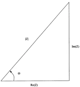
The impedance is most often broken into its real and imaginary forms. A series of useful equations is based on the geometry of Figure 2-4.

Re(Z) Z' Z

J

e

Impedance spectroscopy is only useful when there is a linear response; however, most systems are non-linear. The amplitude of the applied potential difference must be less than the thermal voltage, V = k. At room temperature a linear response

Izi

Im(Z)

Re(Z)

Figure 2-4: Impedance Relationships

for a coated system ± 25 mV is utilized. If the coated system has not undergone too much corrosion it can be considered a linear system and the larger AC signal of ± 25 mV is possible [3]. The larger signal decreases the scatter in the recorded data. Thus this technique is characterized by its small AC fluctuations, which also maintains a measure of a non-destructive testing technique. [33]

The impedance data is relatively simple to generate, and the results can be cor-related with many of the complex material variables of the test system. The data is either analyzed with a mathematical model [34] or an empirical equivalent circuit. Conversely, there is a lot of ambiguity in interpretation of the data. For any given set of data, a number of different equivalent circuits may fit, [33] and from these different circuits, different parameter values yield different information about the actual, phys-ical system. Thus, it is important to use an equivalent circuit that closely represents this physical system.

Electrochemical impedance spectroscopy can be used for many different applica-tions, but one of primary interest is its use in the study of the corrosion behavior of coated metals. This is not possible through more traditional electrochemical tech-niques such as the ones explained previously, due to their poor detection capabilities

08 04 , 0 04 0 R i2 lkohn) KY' 10-go. R 0' E 2w1RC ~04 0 04 08 12 (kohmn) lo' / (HzI cot [~0 1014 10 K)

Figure 2-5: RC Circuits and Corresponding Impedance Spectra

in low-conductivity media. In this field of study, EIS is used to rate coatings, look at interfacial reactions, quantify coating breakdown, and predict the lifetime of coat-ing/metal systems [3]. The study of coated systems employs not only the complex plane or Nyquist plot, which is the Zim (the reactive component) vs Ze (the resistive component) [35], but also Bode plots. Bode plots show the impedance modulus and the phase angle as a function of frequency. From these Bode diagrams, the resistances and capacitances of the circuit elements, the experimental system's components and reactions, can be determined. These plots are much more sensitive to changes with frequency than the Nyquist plots [3].

While a real corroding system is never a simple equivalent circuit, the best way to describe the interpretation method of equivalent circuits is to start simplistically. A parallel RC circuit and a series RC circuit are the most basic. The circuits and their corresponding plots are shown in Figure 2-5 [35]. The complex plane plot of a series

r r gt-i . -45

1~

-RC circuit is a vertical line. The corresponding Bode plot of modulus is a horizontal line in the high frequency range switching to a linear curve with a slope of -1 at lower frequencies. The horizontal portion represents the resistor while the slope of -1 is a pure capacitor. The parallel RC circuit has a complex plane plot of a semicircle with a diameter of the resistance. The Bode modulus plot is the reverse of that for the series circuit. The phase plot is close to 90' when the capacitive element is exhibited and an angle close to 00 when the behavior is resistive. [35]

The more complex behavior of a corroding coated system is built upon these basic circuits. A coated system must take into account the solution resistance, RQ, pore resistance in the coating, Rpo, the capacitance of the film, Cc, the double layer capacitance at the interface, Cdl, and the resistance of the charge transfer at the interface, Rt sometimes taken as the polarization resistance. These last two are attributed to the metal. Another complicating factor that must be accounted for is the possibility of diffusion within the system. This is usually represented by a Warburg impedance. In the complex plane plot this is commonly manifested as a tail at the low frequency end of the semicircle which exhibits a 450 angle [35] for a sample with a planar surface.

An example of the spectra for a coated sample and equivalent circuit can be seen in Figure 2-6 [3]. The equivalent circuit shown here has the following elements: RQ which is the solution resistance, Rpo the pore resistance, Rp the polarization resistance, C, the coating capacitance, and Cdl the double layer capacitance at the metal/coating

interface where corrosion occurs. The capacitance of the polymer is defined by

cc = _Cd d(2.12)

where E is the dielectric constant of the polymer and Eo is the dielectric constant of free space, A is the exposed area of the working electrode, and d is the thickness of the coating. Most impedance models for coated systems are similar to this equivalent circuit, perhaps with more complicated elements embedded in the circuit such as a Warburg impedance. The corresponding Bode plot in Figure 2-6 presents the

modu-C, Rrj R. 106 -90 -80 701 104:- 60 50 -140 102 30 -420 10 100 10-2 100 102 104 106 108 (b) Frequency/Hz

Figure 2-6: Equivalent Circuit and Corresponding Bode Plots for Coated System

lus of the impedance and the phase angle over the measured frequency range. From this plot the values for the circuit are determined. In the modulus representation the plateaus represent resistance and the linear portions with a slope of -1 represent ca-pacitances. The component termed R, is actually Rct, the charge transfer resistance, but it can be related to the polarization resistance, and thus the corrosion rate. The coated system shown here has two time constants, -r = RC, represented as peaks in the phase spectra. The time constant at the high frequency contains information about the polymer coating and the time constant at the low frequency contains in-formation about the metallic substrate. The high frequency resistive plateau is RQ, the mid-frequency one corresponds to Rn + R,,, and the low frequency plateau is Rn + R], + R,. Taking the difference of the latter two yields the R, value which

can be related to the corrosion curent and the mass lost by the system. The first capacitive portion of the modulus plot gives information on Cc, while the second does

When studying a coated system, the impedance spectra changes with time. Ini-tially an intact coating can be detected. Subsequently, water and ionic species diffuse through the polymer. This will lead, ultimately, to corrosion initiation. Once the corrosion of the metal begins, the El spectra can exhibit significant variations. This is dependent on the type of corrosion that occurs and whether it is accompanied

by delamination or not. From the data, corrosion rates can be estimated, using

de-termination of Rp and the charge transfer resistance. The dede-termination of rates is not, however, as simple as those performed with DC techniques, and care must be taken to understand the corroding system during interpretation of the data [30]. The main benefit of EIS relative to DC tests is that EIS measurements have a frequency component which can provide mechanistic information [2].

2.6

Experimental Setup

The electrochemical measurements performed in this study were of two types: DC and AC. The DC tests performed were potentiodynamic and potentiostatic scans

and linear polarization. The AC tests performed were electrochemical impedance spectroscopy.

2.6.1

Samples

There were two main types of samples studied: coated metal and non-coated metal. Within each sample type there were two categories, foils and wafers. The metal of choice was cobalt. Cobalt was chosen because of its magnetic properties. The foils used were 0.25 mm thick, 99.95% pure in an as-rolled condition from Alpha Esar. The wafer samples were 10 cm diameter silicon wafers with an e-beam deposited layer of 99.95% pure cobalt from a target produced by Pure Tech, Inc. The wafer samples were made by the Microsystems Technology Laboratory (MTL) at MIT. The depth of the cobalt coating on the wafers was measured by profilometry on a Tencor-KLA P10. First kapton tape was placed on a monitor silicon wafer before cobalt deposition. After the cobalt was deposited, the tape was removed and the depth difference was

measured. The thickness was determined to be 3200 A. This thickness, while thicker than that used in most microelectronics, was chosen to avoid problems with sheet resistance, which is known to cause ohmic error during electrochemical testing [28].

A polymer coating was then applied to some of the samples. The foil and wafer

samples were coated with a transparent acrylic varnish. The varnish was mixed from Viacryl VSC 5754/60 and Maprenal MF800 both from Vianova Resins. Viacryl is an acrylic emulsion of 60% acrylic in butylacetate. Maprenal is a melamine-formaldehyde of 72% MF in iso-butanol. The mix ratio was 36 g MF to 100 g of resin. Acetone was added to the mixture to produce the right amount of fluidity before application. Greater amounts of acetone were utilized to make the varnish more fluid during application, decreasing the thickness of the polymer. The samples were then dipped into a bath of the varnish and allowed to air dry for a short time prior to curing in an oven at 150 "C for 30 minutes. The curing time was systematically altered to provide a different defect density in the coatings. Thus, the time to coating failure could be decreased and the corrosion initiation rate increased. By lowering the cure time, the number of cross-links formed decreased, making the polymer more permeable to moisture and ions. Thus the undercured polymer was more readily attacked by the test solutions. The thickness of the coating on the foils was measured with a magnetic induction coating thickness measurement system. The range of thicknesses was

15-30 pm. The wafer samples were unable to be measured in this fashion due to their

composite nature. They were coated at the same time and in the same manner as the foils and the thickness was assumed to be the same.

A number of wafer samples were coated with a polyimide coating. This process

was also performed by MTL. The polyimide used was Pyralin PI 2556 from DuPont. The coating process consisted of a spin-coating process followed by a soft bake and then a cure cycle. This cure is the imidization reaction and should be performed in a controlled environment oven free from oxygen which could cause oxidation of the metal substrate at high temperatures. The temperature of the acrylic varnish was sufficiently low to avoid this problem. The polyimide can be fully cured at 180 "C, but higher temperatures are used to achieve the best electrical and mechanical properties

Figure 2-7: SEM Cross Section of PI-Coated Cobalt-Silicon Wafer

of the polymer. A cross section of a polyimide coated wafer sample is shown in Figure

2-7. Three distinct layers are visible; the dark upper layer is the PI coating, the thin

bright layer in the middle is the cobalt, and the large lower layer is the silicon wafer. This image was taken of a sample that was fragmented in liquid nitrogen and then viewed by SEM.

The samples, bare or coated, were sectioned into pieces approximately 1.5 cm by 1.2 cm. The foils were cut with scissors while the wafers were cut with a scribe and snap technique. The silicon side of the wafer sample was marked using a carbide scribe. A small amount of force was then applied to the sample to snap the piece at the scribe mark.

For electrochemical testing the samples needed to have a wire attached for con-nection with the equipment. A thin copper wire with an insulating sheath was used. At the attachment point the wire was stripped and then adhered to the metal surface using either silver epoxy or silver paint. The silver epoxy provided a better mechani-cal bond while the silver paint allowed for a quicker dry time. For the coated samples a region of the polymer was removed prior to wire attachment. For samples using

silver paint, a small amount of 5-minute epoxy was then applied to the attachment region for more stability. And finally a grey paint, Ameron's Amercoat 90, which is a mixture of a resin and cure in a 4:1 volume ratio, was applied to the wire attachment area as well as edges or discontinuities to avoid any unnecessary regions in which localized corrosion could occur.

2.6.2

Electrochemical Cell

The electrochemical cell utilized a three-electrode system. The working electrode was the cobalt sample. The auxiliary or counter electrode was a piece of platinum foil, and the reference was a saturated calomel electrode (SCE). This electrode is a solution of mercurous chloride, Hg₂Cl2, and liquid mercury in contact with a saturated

potassium chloride, KCl, solution. A platinum wire in the mercury allows for an electrical contact. The corresponding half-cell reaction with this electrode is

Hg2Cl2 + 2e- < 2Hg +

2CL-All potentials reported here were measured with respect to this electrode. This

elec-trode has a potential of +0.241 V vs. SHE. SHE is a standard hydrogen elecelec-trode which has a potential defined as 0.00 V for the reaction

2H-+ _{2e- + H}

2

For the potentiodynamic and potentiostatic experiments, the reference electrode was in a separate vessel from the working electrode. The connection was made with a solution bridge and a Luggin probe, similar to the setup in Figure 2-3. For the

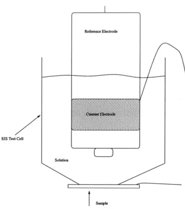
EIS experiments, the counter electrode was wrapped around the working electrode

and they were placed directly into the solution that was in contact with the working electrode, as demonstrated by Figure 2-8. The vessel used for the EIS experiments was a 60 ml syringe with the tip cut off. This provided an area small enough for the sample size, and a volume large enough to contain the electrolyte solution and the

Reference Electrode

EIS Test Cell

Solution

SMIp

Figure 2-8: EIS Test Cell

other two electrodes.

Two test solutions were used-0.5 M NaCl and acidified NaCl. The solutions were made up from reagent grade NaCl and DI water in volumetric flasks. The second solution was made with HCl and the base NaCl solution. The solution was adjusted to a pH in the range of 2-3.

2.6.3

Equipment

Potentiostatic and Potentiodynarnic Scans

For the potentiodynamic and potentiostatic scans, as well as the linear polarization tests, the potentiostat used was a Schlumberger Solartron 1286 Electrochemical In-terface. The potentiostat was joined to a PC by an IEEE/GPIB connection. The scans were performed using the electrochemical software, DC Corrware from Scribner Associates. The majority of the analysis was carried out using this same software or in Microsoft Excel.

Electrochemical Impedance Spectroscopy

The EIS tests were carried out with a Schlumberger Solartron 1287 Electrochemical Interface and a Solartron 1260 Impedance/Gain-Phase Analyzer joined to a computer through an IEEE/GPIB connection. The software used to perform tests was ZPlot and the corresponding analysis package ZView, both from Scribner Associates.

2.7

Results and Discussion

2.7.1

Potentiodynamic and Potentiostatic Scans

The polarization curves for the cobalt samples were performed either in 0.5 M NaCl or in the same solution acidified with HCl to a pH in the range of 2-3. Potentiodynamic curves were generated at a scan rate of 1 mV/s. Before beginning the scan, the open circuit potential of the solution was monitored for at least 10 minutes after sample immersion. Scans were initiated in the cathodic region about -250 mV relative to the corrosion potential and continued into the anodic region to a potential of 700 mV with respect to the reference electrode. Representative curves for both a foil sample and a wafer sample in 0.5 M NaCl are shown in Figure 2-9. Figure 2-10 presents polarization curves for foil samples in the two different electrolytes. Table 2.1 lists the corrosion potential, Ecorr, the corrosion current, Icorr, and the anodic and cathodic Tafel constants, 0,a amd , _{for the three different sample types: wafer in 0.5 M NaCl,}

foil in acidified NaCl, and foil in 0.5 M NaCl.

Sample Ecorr Icorr #a #c

wafer in 0.5 M NaCl -350 mV 1.8 e 5 A 60 mV/decade 180 mV/decade

foil in acidified solution -260 mV 4.1 e- A 40 mV/decade 170 mV/decade

foil in 0.5 M NaCl -370 mV 1.7e- 6 A 70 mV/decade 160 mV/decade

Table 2.1: Electrochemical Data

The potentiodynamic curves for the foil and wafer samples are presented in both Figure 2-9 and Figure 2-10 An example of corroded surface can be seen in Figure 2-12.

Potentiodynamic Polarization Curve 0.8- .6- 0.4- 0.2--o- Co Wafer -U-Co Foil -0.2- -0.4--0.6

-1.006-07 1.00E-06 1.00E-05 1.00E-04 1.OOE-03 1.00E-02 1. OE-01 O OE+00

Current (Amps)

Figure 2-9: Polarization Curves in 0.5 M NaCl for Foil and Wafer Cobalt Samples

The curve for the silicon wafer with deposited cobalt, exhibits a decrease in current in the potential range -240 to -100 mV, which is a tendency towards passivation. This was also noticed in some nickel-cobalt alloy thin films and bulk samples by other researchers [6]. The passive film that is likely formed here is quickly dissolved as the curve returns to an active state. At higher potentials, the current for the wafer sample decreases again, above 190 mV. This is likely due to the removal of most of the cobalt layer, revealing the silicon substrate. Upon completion of such a potentiodynamic scan, the mass loss for the wafer samples was in the range of 60% and the silicon substrate was visible in some regions. Some wafer samples were prepared with cobalt deposited to a thickness of 300

A.

3200 Asamples. It was determined that these samples would not be the most suitable

for use in this project.

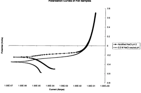
Polarization Curves of Foil Samples 0.8 0.6 0.4 0.2 -*- Acidified NaC pH 2 -- 0.5 M NaC1 neutral pH -0.2 -0.4 -0.8 j-0.8

1.OOE-07 1.OOE-06 1.00E-05 1.00E-04 1.00E-03 1.00E-02 1.OE-01 1.00E+00

Current (Amps)

Figure 2-10: Polarization Curves for Cobalt Foil Samples in Both Solutions

are in the region of -360 mV to -380 mV vs. SCE. From these plots, Tafel slopes were also calculated. These are 70 +15 mV/decade for the anodic region and 160 +15 mV/decade for the cathodic region. These values are in reasonably good agreement with values reported in the literature [36]. It should be noted that there is a slight difference in the corrosion potential between the cobalt wafers and the cobalt foils. There is a more considerable difference in the current, both the corrosion current and the current corresponding to voltages greater than -200 mV. These differences are due to the thickness of the material as well as the structure. The wafer samples have a deposited cobalt layer which has some oxide content, as well as a smaller grain size

[36]. This grain size can cause more homogeneous properties in the material. The

corrosion potential for cobalt on silicon wafers is about -350 mV vs. SCE while the Tafel slopes are 60 +10 mV/decade in the anodic and 180 +10 mV/decade in the cathodic regions. It should be noted that the numbers reported here and the plots are in current, not current density. While the dimensions of all the samples used in these

potentiodynamic tests were the same, the surface area of the wafer and foil samples are different. This is due to the surface roughness of the foil samples.

It can also be seen in Figure 2-10 that there is a change in the corrosion potential and corrosion current with a change in the electrolyte solution. This is due to the pH difference of the electrolytes, as well as the difference in concentration of chloride ions which affect the equilibrium of the anodic and cathodic reactions. In the acidified solution Ecor, is -260 mV vs. SCE and the Tafel constants are 40 mV/decade and 170 mV/decade for the anodic and cathodic regions, respectively. The corrosion rate in the acidified solution is greater than in the neutral NaCl solution, and the corrosion potential is more negative.

Some cobalt wafer samples were tested in the 0.5 M NaCl solution yielding good results, while others did not. In the acidified solution, however, all the wafer samples behaved in an unusual manner. About 3 minutes after immersion, during an open circuit potential test the cobalt started to peel and flake off of the wafer. Some of the wafer samples showed similar behavior in the 0.5 M NaCl solution, even in DI water. This could be an artifact of the cobalt deposition process, or the bond between the cobalt and the silicon could have been aggressively attacked by the acidic solution. The most probable scenario is that the cobalt is poorly adhered to the wafer and the deposited cobalt layer is under stress such that the moisture upsets the precarious system, causing the cobalt layer to delaminate. All subsequent tests were performed solely in the 0.5 M NaCl solution, with the batch of wafers that exhibited no delamination when exposed to this environment.

Potentiostatic scans were carried out on both types of samples. These scans were performed at a specific potential and recorded the current with time. An example of a potentiostatic scan of a foil is presented in Figure 2-11. This reveals the change in current with time, and was performed at -170 mV vs. SCE, in the anodic region with respect to Ecorr,. The curve appears to plateau at a reasonably level current after a short period of time. This would indicate that the corrosion rate for this scan is quite constant.

Potentlostatic Scan 1,20E-01 1.OOE-01 8 OOE-02 S, 6.OOE-02 4.OOE-02-

2.OOE-02--1.00E+02 1.00E+02 3.OOE+02 5.OOE+02 7.OOE+02 9.OOE+02 1.10E+03 1.30E+03 1.50E+03 Time (a)

Figure 2-11: Potentiostatic Scan Performed at -170 mV vs. SCE

find the area under the curve yields the number of coulombs lost by the sample. In this particular sample 142.9 coulombs were lost. Using the following equation

Ita

M = I(2.13)

nF

yields m, the change in mass, where I is the current, t is time, a is the atomic mass, n is the valence change of the metal in the reaction, and F is Faraday's constant, 96,500 C/equivalent. For cobalt the atomic mass, a, is 58.93 g/mol and the valence change is 2. Thus 0.0436 g of mass were lost by the sample from Figure 2-11.

In some instances, a specific mass loss was desired. Then equation 2.13 was utilized to determine the number of coulombs that needed to be lost by the sample. From that information, the potential and time necessary to run the potentiostatic scan could be approximated from a previously generated polarization curve, such as Figure 2-9.

Figure 2-12 shows a cobalt foil sample that was corroded during a potentiodynamic scan in acidified NaCl; it is representative of most of the samples corroded in this