HAL Id: hal-03213015
https://hal.archives-ouvertes.fr/hal-03213015
Submitted on 30 Apr 2021HAL is a multi-disciplinary open access
archive for the deposit and dissemination of sci-entific research documents, whether they are pub-lished or not. The documents may come from teaching and research institutions in France or abroad, or from public or private research centers.
L’archive ouverte pluridisciplinaire HAL, est destinée au dépôt et à la diffusion de documents scientifiques de niveau recherche, publiés ou non, émanant des établissements d’enseignement et de recherche français ou étrangers, des laboratoires publics ou privés.
Application of sparse grid combination techniques to low
temperature plasmas Particle-In-Cell simulations. Part
2 Electron drift instability in a Hall thruster
L. Garrigues, B. Tezenas Du Montcel, G. Fubiani, B. Reman
To cite this version:
L. Garrigues, B. Tezenas Du Montcel, G. Fubiani, B. Reman. Application of sparse grid combination techniques to low temperature plasmas Particle-In-Cell simulations. Part 2 Electron drift instability in a Hall thruster. Journal of Applied Physics, American Institute of Physics, 2021, 129 (15), pp.153304. �10.1063/5.0044865�. �hal-03213015�
1
Application of Sparse grid combination techniques to low
temperature plasmas Particle-In-Cell simulations. Part 2:
Electron Drift Instability in a Hall thruster
L. Garrigues*, B. Tezenas du Montcel, G. Fubiani, and B. Reman
LAPLACE, Université de Toulouse, CNRS, 31062 Toulouse, France.
Three-dimensional simulations of partially magnetized plasma are real challenges that actually limit the understanding of the discharges operations such as the role of kinetic instabilities using explicit Particle-In-Cell (PIC) schemes. The transition to high performance computing cannot overcome all the limits inherent to very high plasma densities and thin mesh sizes employed to avoid numerical heating. We have applied a recent method proposed in the literature [Ricketson and Cerfon, Plasma Phys. Control. Fusion 59, 024002 (2017)] to model low temperature plasmas. This new approach, namely the sparse grid combination technique, offers a gain in computational time by solving the problem on a reduced number of grid cells hence allowing also the reduction of the total number of macroparticles in the system. We have modeled the example of the two-dimensional electron drift instability which
was extensively studied in the literatureto explain the anomalous electron transport in a Hall
thruster. Comparisons between standard and sparse grid PIC methods show an encouraging gain in the computational time with an acceptable level of error. This method offers a unique opportunity for future three-dimensional simulations of instabilities in partially magnetized low temperature plasmas.
2
I.
Introduction
In a companion paper, we have described a new algorithm capable of accelerating Particle-In-Cell (PIC) model in the context of low temperature plasma (LTP) discharges [1]. It is based on the so called “combination technique” applied to sparse grids. Instead of solving the PIC algorithm on a computational domain constrained in space and time by the electron Debye length and the inverse of plasma frequency, respectively, the new method solves the problem on a hierarchy of computational domain [2]. The benefits associated to that method come from an overall smaller number of grid cells offering a gain in computational time, already for two-dimensional problems. Comparisons between standard and sparse grid PIC simulations for capacitively coupled radio-frequency discharges have resulted in a relative error between the two methods of less than a few percent. Moreover, a significant gain in the computational time has been achieved. We have obtained a speed up of a factor of 4
compared to the same problem resolved with the standard PIC method for 5122 grid cells [1].
The goal of this second paper is to evaluate the sparse grid PIC method in partially magnetized LTPs. We have chosen to apply the algorithm in the context of the Hall thruster modeling. A Hall thruster is utilized on board of geostationary satellites for station keeping [3-6]. It operates by means of an electron current which flows on the azimuthal direction of the cylindrical engine under the actions of an axial DC electric and radial magnetic fields. The magnetic field allows an efficient ionization of the propellant gas for pressure conditions on the order of a few mTorr by increasing the residence time of the electrons in the thruster channel. Its strength is chosen to trap the electrons only. Unmagnetized ions accelerated by the axial electric field provide the thrust.
The Hall thruster discharge falls in the category of partially magnetized LTPs such as magnetrons, Penning cell, End-Hall ion source, etc. (see [7-9] and references therein for
3
details). Measurements have revealed that the low pressure and the large induced collisional mean free path result in the diffusion of electrons across the magnetic field which is not predicted by the classical theory. Partially LTPs are the source of instabilities that are responsible for the so-called electron anomalous transport (see [7-9] for general considerations about the type of instabilities found). In Hall thrusters, a specific instability occurs in the azimuthal (E × B) direction which is the source of a fluctuating azimuthal electric field and plasma density. The origin of the instability is related to the large difference in velocity between electrons (forced to drift in the E × B direction) and unmagnetized ions accelerated by the axial electric field. This instability, named “electron cyclotron drift instability” ECDI or “electron drift instability” EDI, is the result of the coupling between electron Bernstein modes and ion-acoustic waves. The dispersion relation in 2D and 3D has been established for the first time in the literature in the 1970’s by Gary and Sanderson (see [10] and references therein). The transition to a modified ion-acoustic instability has been experimentally investigated by Barrett et al. [11] and analytically studied by Gary and Sanderson [10]. More recently, Cavalier et al. [12-13] and Lafleur et al. [14-16] have solved the dispersion relation for typical Hall thruster conditions.
The EDI has also been characterized using PIC simulations in a 2D plane geometry including azimuthal and axial directions [16-18]. The results have confirmed the existence of a fluctuating azimuthal electric field and plasma density in the MHz frequency-range and an mm wavelength-range, as predicted by theory [17-18]. Moreover, comparisons between the solution of the dispersion relation and PIC simulations have established the sensitivity of the wavelength on the electron Debye length and of the frequency of the instability on the ion plasma frequency, in a way similar to the modified acoustic instability. Calculations have also corroborated the ion-wave trapping as the mechanism responsible for the saturation of the instability. Seven research groups worldwide have reproduced the results of Boeuf and
4
Garrigues [17] to obtain a consensus regarding the PIC results and to discriminate against any artificial results arising from numerical inconsistency [18]. The details of the benchmark conditions can be found online on the Landmark project website [19]. In the benchmark of Refs [17-18], the dynamic of neutrals (and associated collisions) is not described, but a
prescribed source term profile is imposed in order to reach a steady state in time scales of a
few tens of microseconds (compared to a few hundreds of microseconds when the neutral dynamics is resolved [20-22]). We believe that the EDI benchmark constitutes the relevant test to check the validity of the sparse grid PIC algorithm in complex situations. In section II, we recall the initial conditions and input data for the benchmark. In section III, we compare calculation results when standard and sparse PIC methods are used. Section IV is devoted to a critical analysis of the results and to a discussion focusing on the speed-up. Concluding remarks are given in section V.
II.
Benchmark conditions
A. Simulation domain and initial conditions
The two-dimensional domain accounts for the axial and the azimuthal directions and extends to 2.5 cm in both directions to keep a square computational domain (see figure 1). Dimensions are indicated in Table 1. The plasma is composed of electrons and singly-charged xenon ions. We do not consider neutrals and related collisions. Dirichlet conditions are applied along the x direction with a voltage on the left boundary (anode) of 200 V and 0 V applied on the right boundary. Particles reaching left and right boundaries are absorbed and no secondary particles are emitted. Periodic boundaries conditions are used along the y direction meaning that one particle crossing the plane y > (respectively y < 0) returns at a new
5
axial position. This method efficiently reduces the computational time and capture
instabilities whose wavelength is shorter than .
At time zero, positions of electrons and ions are uniformly distributed in the simulation
domain along and between and along . Velocity components of electrons and ions
are sampled from a Maxwellian distribution of initial temperatures and , respectively
[23] (see Table 1 for the specifications of the initial conditions). The initial number of
particle-per-cell Npc has been chosen based on the convergence test of Ref. [17]. For the
standard PIC simulations, grid spacing and time step have been adjusted to resolve the
electron Debye length and the inverse of a fraction of the electron plasma frequency
at steady state.
Physical parameters
Axial length x (cm) 2.5
Azimuthal length y (cm) 2.5
Voltage Ud (V) 200
Current density (A/m2) 150
Axial zone of injection , (cm) 0.25, 1
Axial position of cathode (cm) 2.4
Maximum of magnetic field (G) 75
Axial position of maximum of
magnetic field (cm) 0.75 Physical constants Electron mass (10-31 kg) 9.101 Ion mass (10-25 kg) 2.1887 Initial conditions Plasma density (1016 m-3) 8
6
Electron temperature (eV) 10
Ion temperature (eV) 0.5
Initial parameters (standard PIC method)
Grid spacing (cm) /512
Time step (s) 10-11
Number of particles per cell 20 and 400
Table 1: Physical and numerical initial parameters for the benchmark.
Figure 1: Two-dimensional axial (x) azimuthal (y) simulation domain. The zone of
electron-ion pairs injectelectron-ion between axial positelectron-ions x1 and x2 is shown in grey. Electrons are injected
through the cathode plane (dashed lines) at axial position xc. The y-averaged electron and ion
fluxes at the anode, through the emission plane and through exhaust are named and , respectively.
ionization
region
periodic boundary
periodic boundary
cathode
0 V
200 V
axial direction (x)
azi
mutha
ldir
ecti
on
(y)
anode
electron
emission
+
=
.
⃝
B
7 B. Particle injection
Since no collisions and no ionization are taken into account, an external source of charged
particles must be considered. A prescribed and uniform ionization source term along the
direction has been implemented using the following profile:
for
for or (1)
where . Values of and are indicated in Table 1. The maximum of ion current
density that can be extracted at steady state is:
(2),
being the elementary charge. By imposing , we fix the maximum of ion current density
. In that study we have taken to be 150 A/m2 (and = 1.96× 10²³ m-3 s-1). The ionization
profile is given figure 2. At each time step, the number of electron-ion pairs to be injected is
equal to . Electrons and ions are injected at the same position determined by
the following relation:
(3)
where and are pseudo-random numbers uniformly distributed in the interval [0,1].
For current continuity purposes one can write equality of current at the anode (composed of a large fraction of electrons and a small fraction of ions) and at the cathode (composed only of electrons):
8
(4).
In equation (4), , and are respectively the flux at the anode, the electron and the
ion fluxes at the anode, and the electron flux at the cathode (averaged along y). The electron
flux at the cathode will be composed of a fraction entering into the channel and a fraction
that neutralizes the ion flux . At steady state, = . To achieve this, at each time step,
a balance of particle fluxes is calculated at the anode. If , a quantity of electrons corresponding to that net balance is injected, otherwise, no electron is injected. Electrons are
injected uniformly along at the cathode plane (position xc). Their initial velocity is sampled
from a Maxwellian distribution at the same initial temperature of . Note that, contrary to
References [17-18], we do not impose an averaged zero voltage along direction at the
cathode plane and the potential drop Ud is applied between right and left boundaries.
Figure 2: Axial profiles of ionization source term and radial magnetic field.
C. Radial magnetic field profile
The magnetic field which is normal to the simulation plane has a Gaussian profile in the x direction of the form:
0.0 0.5 1.0 1.5 2.0 2.5 0.0 0.5 1.0 1.5 2.0 Source ter m ( x 10 23 m -3 s -1 ) x (cm) 0 20 40 60 80 Rad ial magn etic fiel d (G )
9
(5)
where is the position of the maximum of magnetic field ( = 0.75 cm) and with = 1 for
and with = 2 for . The coefficients of equation (5) , , and can be
analytically determined (see Appendix 1 of Ref. [17]) from the knowledge of magnetic field at = 0 ( = 6 mT), at ( = 1 mT), and fixing = = 0.625 cm. The magnetic field profile is given in figure 2.
III.
Standard vs sparse grid PIC of EDI
We have performed two sets of PIC calculations, one with the standard method (with a
regular grid) with = 20 and 400, and another one using sparse grids. Initial parameters are
given in Table 1. For the sparse grid cases, we have independently illustrated the effect of
and the grid depth on the results. A first series of calculations has been chosen such that
= 512, corresponding to = 9 (coarse grid) varying from 400 to 2000. A second series of
calculations have been performed with refined sparse grids for = 11, and = 12 (with
= 117). The latter has been chosen to keep the computational time similar between the
standard (with = 400) and the sparse grid with = 12 methods. The time step is the same
for all the calculations. The maximum number = 400 in the calculations with the standard
PIC method has been retained as a convergence criteria after a deep study. Above that number, the differences between results are less than a few percent. We will take the results associated to those specific conditions as the “reference” one.
We show in figure 3 the time evolution of the electron current crossing the thruster
channelthat is a signature of the anomalous electron current. An (E×B) axial current can only
be induced by the interactions between electrons and fluctuating azimuthal electric field. In figure 3a, at the beginning, the shape of the electron current variations is very similar for all
10
the cases. A zoom on a time window when convergence is reached reveals differences in the magnitude of the electron current. In figure 3b, results with the standard method show a
current of around 2 A/m for the reference solution. Not surprisingly, reducing in the
standard PIC method induces a large error on the current associated with a larger fluctuating azimuthal electric field. This is due to the numerical noise induced by a low number of particles that samples the particle distribution functions. The same conclusions have been already obtained when parametric studies were conducted for different number of nodes and number of particle-per-cell in Ref. [17]. The green results of figure 3b shows that the error
using sparse grid diminishes by half with = 400 (which keeps the total number of particles
the same as with the standard PIC method). Increasing to 2000 (and more) and
keeping the same level = 9 only slightly reduces the error. The influence of in sparse
calculations reveals, as for standard PIC calculations, that above a given number of particles,
the solution found is not much affected by an increase of . This confirms the conclusions
of Ricketson and Cerfon [2] regarding the effect of (for different examples than our
study). When the grid spacing becomes thinner, the odd oscillations of current also disappear (for = 11 and = 12). As increases the time variation of the current approaches the one obtained in the reference case conditions.
0 10 20 30 40 0 25 50 75 100 30 32 34 36 38 40 0 1 2 3 4 5 6 Iec 1 (A/m) Time (s) standard PIC Npc = 400 - NT = 1.04x10 8 standard PIC Npc = 20 - NT = 5.24x10 6 sparse PIC N = 9 Npc = 400 - NT = 5.24x10 6 sparse PIC N = 9 Npc = 2000 - NT = 2.62x10 7 sparse PIC N = 11 Npc = 117 - NT = 7.54x10 6 sparse PIC N = 12 Npc = 117 - NT = 1.68x10⁷ (a) Iec 1 (A/m) Time (s) (b)
11
Figure 3: (a) Time evolution of electron current for the standard and sparse PIC methods
with different numerical parameters. (b) Same results for a time window between 30 and 40 microseconds, after convergence.
On axis time-averaged electron density (and associated rms fluctuations) and temperature profiles, together with the axial electric field are reported in figure 4. The time averaging is
made on the last 4 microseconds with = 160 equally distributed time shots. The rms
electron density is calculated through the following relation:
(6)
In eq. (6), the averaging along is made on the nodes. For standard PIC calculations,
quantities are calculated on the nodes using bilinear projections. For comparison, profiles obtained with the sparse PIC approach are reconstructed using the combination technique detailed in Refs. [1], [2] and taken at the coincident points of the regular grid nodes. Standard
PIC calculations with a poor statistic ( = 20) preserve the electron density, electron
temperature and axial electric field profiles calculated with a larger number of but fail to
correctly represent the rms electron density fluctuations in the entire x-axis as we see in figure 4c. The fluctuations of electron density show a rms variation of electron density of ~ 10 % at the peak while the rms level when the number of particle-per-cell is large enough drop to 3 % (see figure 4c). Electron density profile shown in figure 4a is qualitatively reproduced by the sparse PIC approach but differences appear for others quantities. The benefit of using the sparse grid approach is visible on the variation of fluctuating electron density. Calculations
with the sparse grid PIC method with = 9 and = 400 show a reduced error
comparatively to the standard PIC approach with the same total number of particles. Nevertheless, the position of maximum of temperature, density and axial electric field is
12
shifted by 5 mm towards the center of the discharge. Even a slight modification of the position of the region of azimuthal electric field fluctuations has a consequence on the local drop of electron conductivity. Accordingly, the region of potential drop and maximum of axial electric field (as well as the maximum of the electron temperature – see figure 4b) is also
shifted. Increasing to 2000 in the sparse PIC approach does not lead to large
modifications of results.
Increasing to 11 leads to a closer agreement between standard and sparse grid PIC
profiles. Maximum of profiles now coincide with the reference case and an even thinner
sparse grid by increasing to 12 shows similar profiles to the reference case. We remark in
Fig. 4d that the electric field is almost identical above the zone of injection of the electron since electron and ion currents are equal (neutralization) at convergence. The situation in front of the anode is different because electron and ion currents (and consequently electron and ion densities in the anode sheath) are not identical (see below). This difference is not inherent to the sparse grid PIC method but is due to the fact that charged particles current at the anode are the result of electron transport for electrons and relative position of source term and
acceleration for ions. As increases, the axial electric field strength gets closer and closer to
the one calculated with the standard PIC method, specifically in the anode sheath. For = 12, the rms electron density fluctuations are now of the same order as in the calculations with the reference case. Error calculations with the method presented in Refs. [1], [2] show an averaged error of 6.5 %, 20.7 %, 7.4 %, and 7.3 % for electron density, rms fluctuations of electron density, electron temperature and axial electric field, respectively.
13
Figure 4: Time-averaged axial profiles of (a) electron density, (b) electron temperature, (c) rms electron density fluctuations and (d) axial electric field for regular and sparse grid and different numerical parameters.
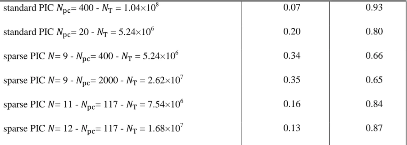
To analyze the consequence of using sparse grid methods, one can compare the ion beam current and the ion current collected at the anode. The source term being imposed, the current
injected along the y-direction is given by 3.75 A/m and . We have
reported in Table 2 the ratio of and . These ratios are influenced by the relative
position of the ionization source term (fixed) and the axial electric field. We notice that for
= 9, shifting the acceleration region towards the exhaust leads to overestimate the ratio
to 35 %, while for = 12 even with a low , this ratio tends to the reference one.
Case 0.0 0.5 1.0 1.5 2.0 2.5 0 10 20 30 40 50 60 0.0 0.5 1.0 1.5 2.0 2.5 0.0 0.5 1.0 1.5 2.0 0.0 0.5 1.0 1.5 2.0 2.5 0.0 0.5 1.0 1.5 2.0 0.0 0.5 1.0 1.5 2.0 2.5 -2 -1 0 1 2 3 4 5 E le c tro n te m p e ra tu re (e V ) n e, rms (1 0 16 m -3 ) x (cm) sparse PIC - N = 9 - Npc = 2000 - NT = 2.62x10⁷ sparse PIC - N = 11 - N pc = 117 - NT = 7.54x10 6 sparse PIC - N = 12 - Npc = 117 - NT = 1.68x10⁷ (c) (d) (b) E le c tro n d e n s ity ( 1 0 17 m -3 ) (a) standard PIC - Npc = 400 - NT = 1.04x10⁸ standard PIC - Npc = 20 - NT = 5.24x10⁶ sparse PIC - N = 9 - Npc = 400 - NT = 5.24x10⁶ x (cm) A x ia l e le c tri c fie ld (1 0 4 V /m )
14 standard PIC = 400 - = 1.04×10⁸ 0.07 0.93 standard PIC = 20 - = 5.24×10⁶ 0.20 0.80 sparse PIC = 9 - = 400 - = 5.24×10⁶ 0.34 0.66 sparse PIC = 9 - = 2000 - = 2.62×10⁷ 0.35 0.65 sparse PIC = 11 - = 117 - = 7.54×10⁶ 0.16 0.84 sparse PIC = 12 - = 117 - = 1.68×10⁷ 0.13 0.87
Table 2: and ratio averaged between 30 and 40 microseconds calculated with
standard and sparse PIC methods for different numerical parameters.
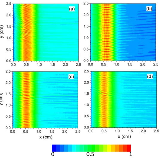
We have plotted 2D profiles of ion density at the same time after convergence in figure 5.
Fig. 5a corresponds to the reference case using the standard PIC approach, with = 400.
From Fig. 5b to 5d sparse grid PIC results are shown with = 9 and = 400, and for =
11 and = 12 with = 117. In Figures 5b, 5c, and 5d, the ion profile has been
reconstructed with the combination technique [1], [2] and shown at coincident grid nodes.
Regardless , the shape of ion density is qualitatively similar to the one calculated with the
standard PIC method. Comparing figures 5a and 5b reveals that amplitude of ion density variation is in the same order but the wavelength of the instability is 35 % larger than the
reference case (see below). Figure 5c shows that an increase of levels ranging from = 9 to
= 11 (and from 17 to 21 sub-grids, respectively) allows us to reproduce accurately the ion density profile in amplitude, the wavelength calculated with the sparse grid being a bit larger
(by 25 %). A continuous increase of to 12 reduces the difference in the wavelength to a
15
Figure 5: 2D profiles of ion density with (a) standard PIC, = 400, (b) sparse grid PIC, =
9 and = 400, (c) sparse grid PIC, = 11 and = 117 and (d) sparse grid PIC = 12
and = 117, using combination technique. Twenty color levels equally spaced are used,
with maximum of (a) 2×10¹⁷ m-3, (b) 2.2×10¹⁷ m-3, (c) 2×10¹⁷ m-3, (d) and 2.2×10¹⁷ m-3.
The FFT along the y direction integrated between x = 0.4 cm and at x = 0.6 cm of the ion
density is plotted in figure 6. As increases, the dominant mode is shifted toward the one
calculated by the standard PIC method ( ~ 8000 rad/m). More interestingly, the effect of the reduction of the noise using sparse PIC approach is clearly visible on the spectrum. Focusing on > 20 000 rad/m, a comparison between the standard and sparse PIC methods (for = 9)
and = 400 shows a reduction between one to two orders of magnitude of the FFT white
noisesignal.
0.0
0.5
1.0
1.5
2.0
2.5
0.0
0.5
1.0
1.5
2.0
2.5
standard
x (cm)
y (cm)
0. 000 1.300E+ 16 2. 600E+ 16 3. 900E+ 16 5. 200E+ 160
0.5
1
16
Figure 6: Fast Fourier Transform of the ion density along the y direction. The signal is integrated between x = 0.4 cm and at x = 0.6 cm. Same conditions as in figure 3.
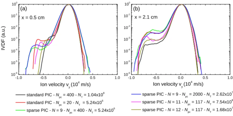
The mechanism associated to the saturation of the instability is the ion wave trapping [14-17]. Ions are trapped by the azimuthal electrostatic wave leading to a broadening of the ion velocity distribution function (IVDF) and the appearance of population of high energetic ions. We have compared the influence of sparse grid PIC approach on the shape of the IVDFs. Figure 7 shows the IVDF integrated in time (same sampling as on-axis profiles of figure 4) and for two locations. The first position is downstream the peak of magnetic field and close to the maximum of ionization source term. At that position, the electron density and the amplitude of oscillations are the highest. The second position is located in the acceleration region where the EDI is convected. We notice that the sparse grid PIC simulations are capable to reproduce what the standard PIC approach gives in terms of ion wave trapping. Specifically, when = 12, the IVDFs look very similar to the ones obtained with the standard PIC method. Very interestingly, the tail of the distribution is well reproduced by sparse grid PIC simulations. 0 5 10 15 20 25 30 35 40 10-3 10-2 10-1 100 101 102
FFT
(a.u.)
Wave number k (10
3rad/m)
standard PIC Npc = 400 - NT = 1.04x10⁸ sparse PIC N = 9 Npc = 400 - NT = 5.24x10⁶ sparse PIC N = 11 Npc = 117 - NT = 7.54x10⁶ sparse PIC N = 12 Npc = 117 - NT = 1.68x10⁷
17
Coming back to the theory of ion-wave trapping [14-17], the maximum of ion velocity in
the azimuthal direction can be written as the sum of the phase and trapped velocities
, where the - being the ion sound speed and
, and are charge and ion mass, respectively, and the rms level of
electric potential field fluctuations. At x = 0.5 cm (fig. 7a), in the region where the ions are generated at rest and axial electric field is very small, the electron temperature is almost the
same for all the calculations and around 25 eV (see fig. 3b) and = 3.5×10⁴ m/s.
at that specific position is the same with, ~ 1 V, for both the standard and sparse grid
PIC simulations when = 12. The trapping velocity is hence 1.7×10⁴ m/s. This simple
estimation gives a maximum velocity reached by the ions of ~ 5×10⁴ m/s in agreement
with results of figure 7a.
At x = 2.1 cm, the electron temperature varies between 10 to 20 eV and between 1.5
and 2.5 V, leading to a maximum velocity between 4.2×10⁴ m/s and 4.8×10⁴ m/s, which
is an underestimation of the maximum ion velocity shown in fig.7b. Nevertheless, in that region the azimuthal drift velocity induced by high axial electric and radial magnetic fields is small and the EDI is certainly the result of non-local phenomena induced by the convection of the instability. Comparisons between the theoretical solution of the modified ion acoustic instability and using the standard PIC approach taking data at that specific position have shown also a deviation in that region [18]. Importantly, sparse PIC approach with refined grid meshes is capable of capturing the IVDF and ion wave trapping phenomena.
18
Figure 7: Time-averaged ion velocity distributions as a function of the azimuthal velocity integrated along the azimuthal direction (a) at x = 0.5 cm ± 0.1 cm and (b) at x = 2.1 cm ± 0.1 cm. Same conditions as in figure 3.
IV.
Discussion
In the context of Hall thrusters, theoretical studies confirmed by the standard PIC simulations have revealed that the Fast Fourier Transform of the spectrum of the density fluctuations generates a spectrum following a dispersion relation that can be derived from a modified ion acoustic instability [14-17]. In particular, the wavelength of the dominant mode
of the instability is ~ 9 . For standard PIC calculations, at the maximum of plasma density
(x = 0.5 cm), ~ 0.5, implying that around 20 points are needed to properly capture the
shape of the EDI. The understanding of the effect of requires a robust numerical analysis
and is let for future studies. Obviously switching from = 9 to = 12 allows us to capture
gradient along the x and y directions with more precision. We can only state that the simulation results are certainly low-pass filtered taking = 9. This affects the wave signal by modifying dominant modes. This filtering effect can be reduced as the level is increased.
In the calculations performed, Poisson equation is solved independently on each of the sparse grids, and the combination technique being used to calculate the electric field at the
-1.0 -0.5 0.0 0.5 1.0 10-6 10-5 10-4 10-3 10-2 10-1 100 -1.0 -0.5 0.0 0.5 1.0 10-6 10-5 10-4 10-3 10-2 10-1 100 sparse PIC - N = 9 - Npc = 2000 - NT = 2.62x10⁷ sparse PIC - N = 11 - Npc = 117 - NT = 7.54x10⁶ sparse PIC - N = 12 - Npc = 117 - NT = 1.68x10⁷ standard PIC - Npc = 400 - NT = 1.04x10⁸ standard PIC - N pc = 20 - NT = 5.24x10 6 sparse PIC - N = 9 - N pc = 400 - NT = 5.24x10 6 Ion velocity vy (104 m/s) (b) x = 2.1 cm IV DF ( a. u. ) x = 0.5 cm Ion velocity vy (104 m/s) (a)
19
particle positions to push them. This is the method used in Ref. [1]. Ricketson and Cerfon [2] have discussed a possible alternative that consists in computing charge densities on the sparse grid nodes (using the standard bilinear interpolation functions), then to perform a projection on the regular grid nodes through the combination technique, and to solve Poisson equation on the regular grid. They argue that using this hybrid approach would reduce the error-grid based in the calculation of the electric field. It seemed interesting to test that “hybrid” method in future calculations. The drawback of the latter is the reduction of the speed-up due to the resolution of the Poisson equation on the regular grid [2]. We also did not vary the time step in the simulations preserving the resolution of a fraction of the inverse of electron plasma density. The question of the Courant-Friedrichs-Lewy (CFL) condition when sparse grid cell changes and becomes smaller is also let for future analysis and studies.
All the simulations have been carried out on the Calmip supercomputer with 5 × Skylake node (Intel Xeon Gold 6140 bi-processors at 2.30 GHz with 18 cores), using Intel compiler version 18.2.199 and IntelMPI version 18.2. The choice of number of nodes has been conducted to optimize the reference case but no particular efforts have been made to independently optimize other calculations. Nevertheless, it can be instructive to see if there is any advantage to use sparse PIC technique to reduce the computational time. We show in
figure 8 the computational time normalized to the reference case (standard approach, 5122 and
= 400). Interestingly, keeping the same number of particles-per-cell offers an advantage
of using sparse PIC technique (gain of factor ~ 6.5). Keeping = 9 and increasing
penalizes the computational time and does not lead to better results. Finally, the generation of more sub-grids leads to an increase of the computational time. The run time of sparse grid
calculations with = 12 and = 117 is the same as in the standard case although the total
number of particles is reduced by a factor 6.5 (see figure 8). This drawback could be addressed by future optimization strategies.
20
We have also carefully looked at the time spent in the sparse PIC subroutines. To summarize, compared to calculations with the standard PIC technique, the time spent to resolve Poisson equation drops since the total number of cells is reduced while the time necessary to compute the charges on the nodes and the different sub-grids increases. This is
consistent with our previous analysis [1]. For = 12 and = 117, the time spent to
compute the charges is almost the same than the time spent to push particles explaining a computational time almost identical to the standard PIC approach. Taking the ratio of number
of cells between the sparse grid method (for = 12) and the regular grid method for =
512 gives 1.8 in our 2D conditions. Same strategy employed for 3D simulations gives a ratio of ~ 70 meaning that using the same approach for future 3D problems would certainly offer a speed-up significantly larger than for 2D simulations.
Figure 8: Speed up (normalized to the reference case, standard method 5122 and = 400) as
a function of total number of particles for the different approaches.
V.
Conclusions
We have used the sparse grid PIC algorithm with the combination technique to demonstrate the applicability of the method to capture the EDI in a Hall Thruster. Focusing on
107 108 0 1 2 3 4 5 6 7 sparse N = 12 - Npc = 117 sparse N = 11 Npc = 117 sparse N = 9 Npc = 2000 standard Npc = 20 Speed up
Total number of particles N
T
standard
Npc = 400 sparse N = 9
21
previous published benchmarks, comparisons between standard PIC and sparse grid methods have been realized. In the calculations with the standard method, the number of grid points
has been chosen to respect constraints on mesh size-to-electron Debye length ratio ( ~
0.5, at maximum of plasma density). Clearly, the construction of the system of grids from the
same power as the standard method (precisely, = 9 corresponding to 29
×29 grid points for the regular grid mesh) offers the advantage of a large speed-up ~ 6.5, but comparisons only
agree with a certain margin. Increasing in the sparse PIC approach does not reduce the
error, meaning that the results tend to be independent of above a certain limit. This has
been observed for the standard PIC simulations in the same context [16] and for sparse grid PIC results in other simulations [1], [2].
One way to reduce the error is to construct a hierarchy of sparse grids from a larger . Doing this, we observe a reduction of the error to typically 20 % for a speed-up of typically 3.
Increasing of one additional level still reduces the error to 7 %, but no gain in
computational time is reached. Further analyses are needed to provide a clear explanation of such effects. Smaller mesh sizes increase the numerical resolution of the gradients in the plasma parameters which results in a reduction of the grid-based error associated with the combination technique. Keeping the same strategy for future 3D simulations with = 12 will offer a gain in the number of cells for the sparse grids of around 70 compared to only 1.8 for 2D. Moreover, the high performance computing techniques for 3D simulations of this new type of explicit scheme have to be revisited (such as the optimizations of charge deposition, of methods to solve Poisson’s equation using sparse matrixes with different geometrical aspects, etc.).
22
Data availability
The data supporting the findings of this study are available from the corresponding author upon reasonable request.
Acknowledgments
This work was supported by the RTRA STAE (Réseau Thématique de Recherche Avancée Sciences et Technologies pour l’Aéronautique et l’Espace) foundation. Part of this work was granted access to the HPC resources of CALMIP supercomputing center under the allocation 2013-P1125. Authors want to thank Mathieu Lobet from Maison de la Simulation for discussions and implementation of SIMD optimization techniques.
23
References
[1] L. Garrigues, B. Tezenas du Montcel, G. Fubiani, F. Bertomeu, F. Deluzet and J. Narski,
submitted (2021).
[2] L. F. Rickeston and A. J. Cerfon, Plasma Physics and Controlled Fusion 59, 024002 (2017).
[3] J. P. Boeuf, Journal Applied Physics 121, 011101 (2017).
[4] S. Mazouffre, Plasma Sources Science and Technology 25, 033002 (2016).
[5] I. Levchenko, K. Bazaka, Y. Ding, Y. Raitses, S. Mazouffre, T. Henning, P. J. Klar, S. Shinohara, J. Schein, L. Garrigues, M. Kim, D. Lev, F. Taccogna, R. W. Boswell, C. Charles, H. Koizumi, S. Yan, C. Scharlemann, M. Keidar, and S. Xu, Applied Physics Reviews 5, 011104 (2018).
[6] I. Levchenko, S. Xu, S. Mazouffre, D. Lev, D. Pedrini, D. Goebel, L. Garrigues, F. Taccogna, and K. Bazaka, Physics of Plasmas 27, 020601 (2020).
[7] A. I. Smolyakov, O. Chapurin, W. Frias, O. Koshkarov, I. Romadanov, T. Tang, M. Umansky, Y. Raitses, I. D. Kaganovich, and V. P. Lakhin, Plasma Physics and Controlled Fusion 59, 014041 (2017).
[8] J. P. Boeuf, Frontiers in Physics 2, 74 (2014).
[9] S. N. Abolmasov, Plasma Sources Science and Technology 21, 035006 (2012).
[10] S. P. Gary, theory of space plasma microinstability, Cambridge University Press (1993). [11] P. J. Barrett, B. D. Fried, C. F. Kennel, J. M. Sellen, and R. J. Taylor, Physical Review Letters 28, 339 (1972).
[12] J. Cavalier, N. Lemoine, G. Bonhomme, S. Tsikata, C. Honoré, and D. Grésillon, Physics of Plasmas 19, 082117 (2012).
[13] J. Cavalier, N. Lemoine, G. Bonhomme, S. Tsikata, C. Honoré, and D. Grésillon, Physics of Plasmas 20, 082107 (2013).
24
[14] T. Lafleur, S. Baalrud, and P. Chabert, Plasma Sources Science and Technology 26, 024008 (2017).
[15] T. Lafleur and P. Chabert, Physics of Plasmas 23, 053503 (2016).
[16] T. Lafleur and P. Chabert, Plasma Sources Science and Technology 27, 015003 (2018). [17] J. P. Boeuf and L. Garrigues, Physics of Plasmas 25, 061204 (2018).
[18] T. Charoy, J. P. Boeuf, A. Bourdon, J. A. Carlsson, P. Chabert, B. Cuenot, D. Eremin, L. Garrigues, K. Hara, I. D. Kaganovich, A. T. Powis, A. Smolyakov, D. Sydorenko, A. Tavant, O. Vermorel, and W. Villafana, Plasma Sources Science and Technology 28, 105010 (2019).
[19] https://www.landmark-plasma.com/ (21 october 2020).
[20] J. C. Adam, A. Héron, and G. Laval, Physics of Plasmas 11, 295 (2004). [21] P. Coche and L. Garrigues, Physics of Plasmas 21, 023503 (2014).
[22] V. Croes, T. Lafleur, Z. Bonaventura, A. Bourdon, and P. Chabert, Plasma Sources Science and Technology 26, 034001 (2017).
[23] L. Garrigues, G. Fubiani, and J. P. Boeuf, Journal of Applied Physics 120, 213303 (2016).