3D Face Recognition Under Expressions,Occlusions and Pose Variations

HAL Id: halshs-00783066

https://halshs.archives-ouvertes.fr/halshs-00783066

Submitted on 31 Jan 2013

HAL is a multi-disciplinary open access

archive for the deposit and dissemination of

sci-entific research documents, whether they are

pub-lished or not. The documents may come from

teaching and research institutions in France or

abroad, or from public or private research centers.

L’archive ouverte pluridisciplinaire HAL, est

destinée au dépôt et à la diffusion de documents

scientifiques de niveau recherche, publiés ou non,

émanant des établissements d’enseignement et de

recherche français ou étrangers, des laboratoires

publics ou privés.

3D Face Recognition Under Expressions,Occlusions and

Pose Variations

Hassen Drira, Ben Amor Boulbaba, Srivastava Anuj, Mohamed Daoudi, Rim

Slama

To cite this version:

Hassen Drira, Ben Amor Boulbaba, Srivastava Anuj, Mohamed Daoudi, Rim Slama. 3D Face

Recog-nition Under Expressions,Occlusions and Pose Variations. IEEE Transactions on Pattern Analysis

and Machine Intelligence, Institute of Electrical and Electronics Engineers, 2013, pp.2270 - 2283.

�halshs-00783066�

3D Face Recognition Under Expressions,

Occlusions and Pose Variations

Hassen Drira, Boulbaba Ben Amor, Anuj Srivastava, Mohamed Daoudi, and Rim Slama

Abstract—We propose a novel geometric framework for analyzing 3D faces, with the specific goals of comparing, matching, and averaging their shapes. Here we represent facial surfaces by radial curves emanating from the nose tips and use elastic shape analysis of these curves to develop a Riemannian framework for analyzing shapes of full facial surfaces. This representation, along with the elastic Riemannian metric, seems natural for measuring facial deformations and is robust to challenges such as large facial expressions (especially those with open mouths), large pose variations, missing parts, and partial occlusions due to glasses, hair, etc. This framework is shown to be promising from both – empirical and theoretical – perspectives. In terms of the empirical evaluation, our results match or improve the state-of-the-art methods on three prominent databases: FRGCv2, GavabDB, and Bosphorus, each posing a different type of challenge. From a theoretical perspective, this framework allows for formal statistical inferences, such as the estimation of missing facial parts using PCA on tangent spaces and computing average shapes.

Index Terms—3D face recognition, shape analysis, biometrics, quality control, data restoration.

✦

1

I

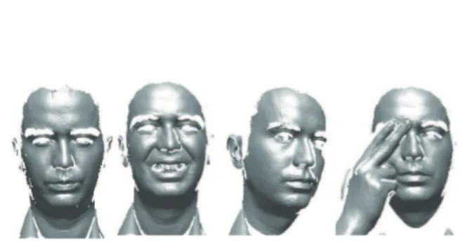
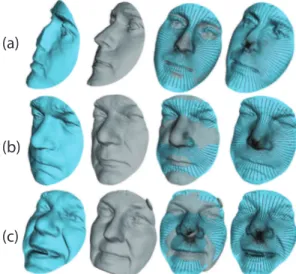
Due to the natural, non-intrusive, and high through-put nature of face data acquisition, automatic face recognition has many benefits when compared to other biometrics. Accordingly, automated face recog-nition has received a growing attention within the computer vision community over the past three decades. Amongst different modalities available for face imaging, 3D scanning has a major advantage over 2D color imaging in that nuisance variables, such as illumination and small pose changes, have a rela-tively smaller influence on the observations. However, 3D scans often suffer from the problem of missing parts due to self occlusions or external occlusions, or some imperfections in the scanning technology. Additionally, variations in face scans due to changes in facial expressions can also degrade face recognition performance. In order to be useful in real-world appli-cations, a 3D face recognition approach should be able to handle these challenges, i.e., it should recognize people despite large facial expressions, occlusions and large pose variations. Some examples of face scans highlighting these issues are illustrated in Fig. 1.

We note that most recent research on 3D face analysis has been directed towards tackling changes in facial expressions while only a relatively modest

This paper was presented in part at BMVC 2010 [7].

• H. Drira, B. Ben Amor and M. Daoudi are with LIFL (UMR CNRS

8022), Institut Mines-T´el´ecom/TELECOM Lille 1, France. E-mail: hassen.drira@telecom-lille1.eu

• R. Slama is with LIFL (UMR CNRS 8022), University of Lille 1,

France.

• A. Srivastava is with the Department of Statistics, FSU, Tallahassee,

FL, 32306, USA.

Fig. 1. Different challenges of 3D face recognition:

expressions, missing data and occlusions.

effort has been spent on handling occlusions and missing parts. Although a few approaches and cor-responding results dealing with missing parts have been presented, none, to our knowledge, has been ap-plied systematically to a full real database containing scans with missing parts. In this paper, we present a comprehensive Riemannian framework for analyzing facial shapes, in the process dealing with large expres-sions, occlusions and missing parts. Additionally, we provide some basic tools for statistical shape analysis of facial surfaces. These tools help us to compute a typical or average shape and measure the intra-class variability of shapes, and will even lead to face atlases in the future.

1.1 Previous Work

The task of recognizing 3D face scans has been approached in many ways, leading to varying levels of successes. We refer the reader to one of many extensive surveys on the topic, e.g. see Bowyer et al. [3]. Below we summarize a smaller subset that is more relevant to our paper.

1. Deformable template-based approaches: There have been several approaches in recent years that rely on deforming facial surfaces into one another, under some chosen criteria, and use quantifications of these deformations as metrics for face recognition. Among these, the ones using non-linear deformations facilitate the local stretching, compression, and bending of surfaces to match each other and are referred to as elastic methods. For instance, Kakadiaris et al. [13] utilize an annotated face model to study geometrical variability across faces. The annotated face model is deformed elastically to fit each face, thus matching different anatomical areas such as the nose, eyes and mouth. In [25], Passalis et al. use automatic landmarking to estimate the pose and to detect occluded areas. The facial symmetry is used to overcome the challenges of missing data here. Similar approaches, but using manually annotated models, are presented in [31], [17]. For example, [17] uses manual landmarks to develop a thin-plate-spline based matching of facial surfaces. A strong limitation of these approaches is that the extraction of fiducial landmarks needed during learning is either manual or semi-automated, except in [13] where it is fully automated.

2. Local regions/ features approaches: Another com-mon framework, especially for handling expression variability, is based on matching only parts or regions rather than matching full faces. Lee et al. [15] use ratios of distances and angles between eight fiducial points, followed by a SVM classifier. Similarly, Gupta et al. [11] use Euclidean/geodesic distances between anthropometric fiducial points, in conjunction with linear classifiers. As stated earlier, the problem of au-tomated detection of fiducial points is non-trivial and hinders automation of these methods. Gordon [10] argues that curvature descriptors have the potential for higher accuracy in describing surface features and are better suited to describe the properties of faces in areas such as the cheeks, forehead, and chin. These descriptors are also invariant to viewing angles. Li et al. [16] design a feature pooling and ranking scheme in order to collect various types of low-level geometric features, such as curvatures, and rank them according to their sensitivity to facial expressions. Along similar lines, Wang et al. [32] use a signed shape-difference map between two aligned 3D faces as an interme-diate representation for shape comparison. McKeon and Russ [19] use a region ensemble approach that is based on Fisherfaces, i.e., face representations are learned using Fisher’s discriminant analysis.

In [12], Huang et al. use a multi-scale Local Binary Pattern (LBP) for a 3D face jointly with shape index. Similarly, Moorthy et al. [20] use Gabor features

around automatically detected fiducial points.

To avoid passing over deformable parts of faces encompassing discriminative information, Faltemier

et al. [9] use 38 face regions that densely cover the face, and fuse scores and decisions after performing ICP on each region. A similar idea is proposed in [29] that uses PCA-LDA for feature extraction, treating the likelihood ratio as a matching score and using the majority voting for face identification. Queirolo et al. [26] use Surface Inter-penetration Measure (SIM) as a similarity measure to match two face images. The authentication score is obtained by combining the SIM values corresponding to the matching of four different face regions: circular and elliptical areas around the nose, forehead, and the entire face region. In [1], the authors use Average Region Models (ARMs) locally to handle the challenges of missing data and expression-related deformations. They manually divide the facial area into several meaningful components and the registration of faces is carried out by separate dense alignments to the corresponding ARMs. A strong limitation of this approach is the need for manual segmentation of a face into parts that can then be analyzed separately. 3. Surface-distance based approaches: There are sev-eral papers that utilize distances between points on facial surfaces to define features that are eventually used in recognition. (Some papers call it geodesic

dis-tance but, in order to distinguish it from our later use

of geodesics on shape spaces of curves and surfaces, we shall call it surface distance.) These papers assume that surface distances are relatively invariant to small changes in facial expressions and, therefore, help gen-erate features that are robust to facial expressions. Bronstein et al. [4] provide a limited experimental illustration of this invariance by comparing changes in surface distances with the Euclidean distances between corresponding points on a canonical face surface. To handle the open mouth problem, they first detect and remove the lip region, and then compute the surface distance in presence of a hole correspond-ing to the removed part [5]. The assumption of preser-vation of surface distances under facial expressions motivates several authors to define distance-based features for facial recognition. Samir et al. [28] use the level curves of the surface distance function (from the tip of the nose) as features for face recognition. Since an open mouth affects the shape of some level curves, this method is not able to handle the problem of missing data due to occlusion or pose variations. A similar polar parametrization of the facial surface is proposed in [24] where the authors study local geometric attributes under this parameterization. To deal with the open mouth problem, they modify the parametrization by disconnecting the top and bottom lips. The main limitation of this approach is the need for detecting the lips, as proposed in [5]. Berretti et al. [2] use surface distances to define facial stripes which, in turn, is used as nodes in a graph-based recognition algorithm.

The main limitation of these approaches, apart from the issues resulting from open mouths, is that they assume that surface distances between facial points are preserved within face classes. This is not valid in the case of large expressions. Actually, face ex-pressions result from the stretching or the shrinking of underlying muscles and, consequently, the facial skin is deformed in a non-isometric manner. In other words, facial surfaces are also stretched or compressed locally, beyond a simple bending of parts.

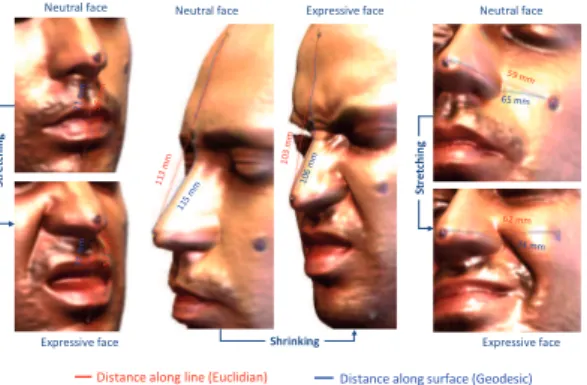
In order to demonstrate this assertion, we placed four markers on a face and tracked the changes in the surface and Euclidean (straight line) distances between the markers under large expressions. Fig. 2 shows some facial expressions leading to a significant shrinking or stretching of the skin surface and, thus, causing both Euclidean and surface distances between these points to change. In one case these distances decrease (from 113 mm to 103 mm for the Euclidean distance, and from 115 mm to 106 mm for the surface distance) while in the other two cases they increase. This clearly shows that large expressions can cause stretching and shrinking of facial surfaces, i.e., the facial deformation is elastic in nature. Hence, the assumption of an isometric deformation of the shape of the face is not strictly valid, especially for large expressions. This also motivates the use of elastic shape analysis in 3D face recognition.

7 1 m m 7 7 m m 5 7 m m 56 m m Neutral face S tr e tc h in g Expressive face

Distance along line (Euclidian) Distance along surface (Geodesic)

65 mm 74 mm 62 mm 59 mm Neutral face S tr e tc h in g Expressive face 106 m m 115 mm 113 m m 103 m m Shrinking

Neutral face Expressive face

Fig. 2. Significant changes in both Euclidean and

surface distances under large facial expressions.

1.2 Overview of Our Approach

This paper presents a Riemannian framework for 3D facial shape analysis. This framework is based on elastically matching and comparing radial curves emanating from the tip of the nose and it handles several of the problems described above. The main contributions of this paper are:

• It extracts, analyzes, and compares the shapes of

radial curves of facial surfaces.

• It develops an elastic shape analysis of 3D faces

by extending the elastic shape analysis of curves [30] to 3D facial surfaces.

• To handle occlusions, it introduces an occlusion

detection and removal step that is based on recursive-ICP.

• To handle the missing data, it introduces a

restoration step that uses statistical estimation on shape manifolds of curves. Specifically, it uses PCA on tangent spaces of the shape manifold to model the normal curves and uses that model to complete the partially-observed curves.

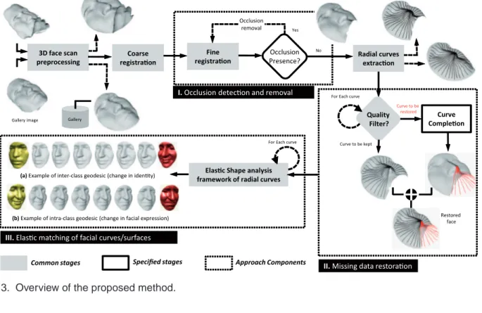
The different stages and components of our method are laid out in Fig. 3. While some basic steps are common to all application scenarios, there are also some specialized tools suitable only for specific situa-tions. The basic steps that are common to all situations include 3D scan preprocessing (nose tip localization, filling holes, smoothing, face cropping), coarse and fine alignment, radial curve extraction, quality filter-ing, and elastic shape analysis of curves (Component

IIIand quality module in Component II). This basic

setup is evaluated on the FRGCv2 dataset following the standard protocol (see Section 4.2). It is also tested on the GAVAB dataset where, for each subject, four probe images out of nine have large pose variations (see Section 4.3). Some steps are only useful where one anticipates some data occlusion and missing data. These steps include occlusion detection (Component

I) and missing data restoration (Component II). In

these situations, the full processing includes

Compo-nents I+II+III to process the given probes. This

ap-proach has been evaluated on a subset of the Bosphorus dataset that involves occlusions (see Section 4.4). In the last two experiments, except for the manual de-tection of nose coordinates, the remaining processing is automatic.

2

R

, E

C

: M

Since an important contribution of this paper is its novel use of radial facial curves studied using elastic shape analysis.

2.1 Motivation for Radial Curves

Why should one use the radial curves emanating from the tip of the nose for representing facial shapes? Firstly, why curves and not other kinds of facial features? Recently, there has been significant progress in the analysis of curves shapes and the resulting algorithms are very sophisticated and efficient [30], [33]. The changes in facial expressions affect different regions of a facial surface differently. For example, during a smile, the top half of the face is relatively unchanged while the lip area changes a lot, and when a person is surprised the effect is often the opposite. If chosen appropriately, curves have the potential to capture regional shapes and that is why their role becomes important. The locality of shapes represented by facial curves is an important reason

3D face scan preprocessing Probe image Gallery image Coarse registra!on Radial curves extrac!on Gallery Fine registra!on Occlusion Presence? Occlusion removal Yes No Quality Filter? For Each curve

Curve to be kept Curve to be restored Curve Comple!on Restored face Elas!c Shape analysis

framework of radial curves

III. Elas!c matching of facial curves/surfaces (a) Example of inter-class geodesic (change in iden!ty)

(b) Example of intra-class geodesic (change in facial expression)

II. Missing data restora!on I. Occlusion detec!on and removal

Common stages Specified stages Approach Components

For Each curve

Fig. 3. Overview of the proposed method.

Fig. 4. A smile (see middle) changes the shapes of the curves in the lower part of a the face while the act of surprise changes shapes of curves in the upper part of the face (see right).

for their selection. The next question is: Which facial curves are suitable for recognizing people? Curves on a surface can, in general, be defined either as the level curves of a function or as the streamlines of a gradient field. Ideally, one would like curves that maximally separate inter-class variability from the intra-class variability (typically due to expression changes). The past usage of the level curves (of the surface distance function) has the limitation that each curve goes through different facial regions and that makes it difficult to isolate local variability. Actually, the previous work on shape analysis of facial curves for 3D face recognition was mostly based on level curves [27], [28].

In contrast, the radial curves with the nose tip as origin have a tremendous potential. This is because: (i) the nose is in many ways the focal point of a face. It is relatively easy and efficient to detect the nose tip (compared to other facial parts) and to extract radial curves, with nose tip as the center, in a

com-pletely automated fashion. It is much more difficult to automatically extract other types of curves, e.g. those used by sketch artists (cheek contours, fore-head profiles, eye boundaries, etc). (ii) Different radial curves pass through different regions and, hence, can be associated with different facial expressions. For instance, differences in the shapes of radial curves in the upper-half of the face can be loosely attributed to the inter-class variability while those for curves passing through the lips and cheeks can largely be due to changes in expressions. This is illustrated in Fig. 4 which shows a neutral face (left), a smiling face (middle), and a surprised face (right). The main difference in the middle face, relative to the left face, lies in the lower part of the face, while for the right face the main differences lie in the top half. (iii) Radial curves have a more universal applicability. The curves used in the past have worked well for some specific tasks, e.g., lip contours in detecting certain expres-sions, but they have not been as efficient for some other tasks, such as face recognition. In contrast, radial curves capture the full geometry and are applicable to a variety of applications, including facial expression recognition. (iv) In the case of the missing parts and partial occlusion, at least some part of every radial curve is usually available. It is rare to miss a full radial curve. In contrast, it is more common to miss an eye due to occlusion by glasses, the forehead due to hair, or parts of cheeks due to a bad angle for laser reflection. This issue is important in handling the missing data via reconstruction, as shall be described later in this paper. (v) Natural face deformations

are largely (although not exactly) symmetric and, to a limited extent, are radial around the nose. Based on these arguments, we choose a novel geometrical representation of facial surfaces using radial curves that start from the nose tip.

2.2 Motivation for Elasticity

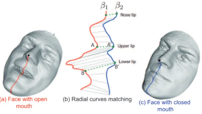
Consider the two parameterized curves shown in Fig.

5; call them β1 and β2. Our task is to automatically

match points on these radial curves associated with two different facial expressions. The expression on the left has the mouth open whereas the expression on the right has the mouth closed. In order to compare their shapes, we need to register points across those curves. One would like the correspondence to be such that geometric features match across the curves as well as possible. In other words, the lips should match the lips and the chin should match the chin. Clearly, if we force an arc-length parameterization and match points that are at the same distance from the starting point, then the resulting matching will not be optimal.

The points A and B on β1 will not match the points

A’ and B’ on β2 as they are not placed at the same

distances along the curves. For curves, the problem of optimal registration is actually the same as that of optimal re-parameterization. This means that we need to find a re-parameterization function γ(t) such that

the point β1(t) is registered with the point β2(γ(t)),

for all t. The question is how to find an optimal γ for

an arbitrary β1 and β2? Keep in mind that the space

of all such γs is infinite dimensional because it is a space of functions.

As described in [30], this registration is accom-plished by solving an optimizing problem using the dynamic programming algorithm, but with an objec-tive function that is developed from a Riemannian metric. The chosen metric, termed an elastic metric, has a special property that the same re-parameterization of two curves does not change the distance between them. This, in turn, enables us to fix the parameter-ization of one curve arbitrarily and to optimize over the parameterization of the other. This optimization leads to a proper distance (geodesic distance) and an optimal deformation (geodesic) between the shapes of curves. In other words, it results in their elastic comparisons. Please refer to [30] for details.

2.3 Automated Extraction of Radial Curves

Each facial surface is represented by an indexed col-lection of radial curves that are defined and extracted as follows. Let S be a facial surface obtained as an output of the preprocessing step. The reference curve on S is chosen to be the vertical curve after the face has been rotated to the upright position. Then, a radial

curve βα is obtained by slicing the facial surface by a

plane Pαthat has the nose tip as its origin and makes

an angle α with the plane containing the reference

(a) Face with open mouth

(b) Radial curves matching _{(c) Face with closed} mouth

A A’

B

B’

Fig. 5. An example of matching radial curves extracted from two faces belonging to the same person: a curve with an open mouth (on the left) and a curve with a closed mouth (on the right). One needs a combination of stretching and shrinking to match similar points (upper lips, lower lips, etc)

curve. That is, the intersection of Pαwith S gives the

radial curve βα. We repeat this step to extract radial

curves from S at equally-separated angles, resulting in a set of curves that are indexed by the angle α. Fig. 6 shows an example of this process.

If needed, we can approximately reconstruct S from

these radial curves according to S≈ ∪αβα = ∪α{S ∩

Pα}. In the later experiments, we have used 40 curves

to represent a surface. Using these curves, we will demonstrate that the elastic framework is well suited to modeling of deformations associated with changes in facial expressions and for handling missing data.

Fig. 6. Extraction of radial curves: images in the middle illustrate the intersection between the face surface and planes to form two radial curves. The collection of radial curves is illustrated in the rightmost image.

In our experiments, the probe face is first rigidly aligned to the gallery face using the ICP algorithm. In this step, it is useful but not critical to accurately find the nose tip on the probe face. As long as there is a sufficient number of distinct regions available on the probe face, this alignment can be performed. Next, after the alignment, the radial curves on the

probe model are extracted using the plane Pαpassing

through the nose tip of the gallery model at an angle

α with the vertical. This is an important point in

that only the nose tip of the gallery and a good alignment between gallery-probe is needed to extract good quality curves. Even if some parts of the probe

face are missing, including its nose region, this process can still be performed. To demonstrate this point, we take session #0405d222, from the FRGCv2 dataset, in which some parts of the nose are missing and are filled using a linear interpolation filter (top row of Fig. 7). The leftmost panel shows the hole-filled probe face, the next panel shows the gallery face, the third panel shows its registration with the gallery face and extracted curves on the gallery face. The last panel shows the extracted curves for the probe face. As shown there, the alignment of the gallery face with the probe face is good despite a linear interpolation of the missing points. Then, we use the gallery nose coordinates to extract radial curves on the probe surface. The gallery face in this example belongs to the same person under the same expression. In the second row, we show an example where the two faces belong to the same person but represent different expressions/pose. Finally, in the last row we show a case where the probe and the gallery faces belong to different persons. Since the curve extraction on the probe face is based on the gallery nose coordinates which belongs to another person, the curves may be shifted in this nose region. However, this small inaccuracy in curve extraction is actually helpful since it increases the inter-class distances and improves the biometric performance.

(a)

(b)

(c)

Fig. 7. Curves extraction on a probe face after its

rigid alignment with a gallery face. In (a), the nose region of the probe is missing and filled using linear interpolation. The probe and gallery faces are from the same class for (a) and (b), while they are from different classes for (c).

2.4 Curve Quality Filter

In situations involving non-frontal 3D scans, some curves may be partially hidden due to self occlu-sion. The use of these curves in face recognition can severely degrade the recognition performance and, therefore, they should be identified and discarded. We

Discarded curves Retained curves

Fig. 8. Curve quality filter: examples of detection of broken and short curves (in red) and good curves (in blue).

introduce a quality filter that uses the continuity and the length of a curve to detect such curves. To pass the quality filter, a curve should be one continuous piece and have a certain minimum length, say of, 70mm. The discontinuity or the shortness of a curve results either from missing data or large noise.

We show two examples of this idea in Fig. 8 where we display the original scans, the extracted curves, and then the action of the quality filter on these curves. Once the quality filter is applied and the high-quality curves retained, we can perform face recogni-tion procedure using only the remaining curves. That is, the comparison is based only on curves that have passed the quality filter. Let β denotes a facial curve, we define the boolean function quality: (quality(β) = 1) if β passes the quality filter and (quality(β) = 0) otherwise. Recall that during the pre-processing step, there is a provision for filling holes. Sometimes the missing parts are too large to be faithfully filled using linear interpolation. For this reason, we need the quality filter that will isolate and remove curves associated with those parts.

3

S

A

F

S

In this section we will start by summarizing a recent work in elastic shape analysis of curves and extend it to shape analysis of facial surfaces.

3.1 Background on the Shapes of Curves

Let β : I → R3_{, represent a parameterized curve on}

the face, where I = [0, 1]. To analyze the shape of β, we shall represent it mathematically using the

square-root velocity function (SRVF) [30], denoted by q(t) =

˙ β(t)

√

| ˙β(t)|; q(t) is a special function of β that simplifies

computations under elastic metric. More precisely, as shown in [30], an elastic metric for comparing shapes

of curves becomes the simple L2_{-metric under the}

SRVF representation. (A similar metric and represen-tation for curves was also developed by Younes et

al. [33] but it only applies to planar curves and not to facial curves). This point is very important as it simplifies the analysis of curves, under the elastic met-ric, to the standard functional analysis. Furthermore,

under L2_{-metric, the re-parametrization group acts by}

isometries on the manifold of q functions, which is not the case for the original curve β. To elaborate on the last point, let q be the SRVF of a curve β. Then, the

SRVF of a re-parameterized curve β◦ γ is given by

√

˙γ(q ◦ γ). Here γ : I → I is a re-parameterization function and let Γ be the set of all such functions.

Now, if q1 and q2 are SRVFs of two curves β1 and

β2, respectively, then it is easy to show that under the

L2 norm, kq1− q2k = k√˙γ(q1◦ γ) −√˙γ(q2◦ γ)k, for

all γ ∈ Γ, while kβ1− β2k 6= k(β1◦ γ) − (β2◦ γ)k in

general. This is one more reason why SRVF is a better representation of curves than β for shape analysis.

Define the pre-shape space of such curves:C = {q :

I→ R3_{| kqk = 1} ⊂ L}2_{(I, R}3_{), where k·k implies the}

L2 norm. With the L2 _{metric on its tangent spaces, C}

becomes a Riemannian manifold. Also, since the

ele-ments ofC have a unit L2_{norm,C is a hypersphere in}

the Hilbert space L2_{(I, R}3_{). Furthermore, the geodesic}

path between any two points q1, q2∈ C is given by the

great circle, ψ : [0, 1]→ C, where

ψ(τ ) = 1

sin(θ)(sin((1 − τ)θ)q1+ sin(θτ )q2) , (1)

and the geodesic length is θ = dc(q1, q2) =

cos−1(hq1, q2i).

In order to study shapes of curves, one should iden-tify all rotations and re-parameterizations of a curve as an equivalence class. Define the equivalent class of

qas: [q] = closure{p ˙γ(t)Oq(γ(t))|O ∈ SO(3), γ ∈ Γ}.

The set of such equivalence classes, denoted by S =.

{[q]|q ∈ C} is called the shape space of open curves

in R3_{. As described in [30], S is a metric space with}

the metric inherited from the larger spaceC. To obtain

geodesics and geodesic distances between elements of S, one needs to solve the optimization problem:

(O∗, γ∗) = argmin

(O,γ)∈SO(3)×Γ

dc(q1,p ˙γO(q2◦ γ)). (2)

For a fixed O in SO(3), the optimization over Γ is done using the dynamic programming algorithm

while, for a fixed γ∈ Γ, the optimization over SO(3)

is performed using SVD. By iterating between these two, we can reach a solution for the joint

optimiza-tion problem. Let q∗

2(t) =

q ˙

γ∗_(t)O∗_q

2(γ∗(t))) be the

optimal element of [q2], associated with the optimal

rotation O∗ _{and re-parameterization γ}∗ _{of the second}

curve, then the geodesic distance between [q1] and [q2]

in S is ds([q1], [q2]) = d. c(q1, q2∗) and the geodesic is

given by Eqn. 1, with q2 replaced by q2∗.

3.2 Shape Metric for Facial Surfaces

Now we extend the framework from radial curves to full facial surfaces. A facial surface S is represented by

an indexed collection of radial curves, indexed by the

nuniform angles A = {0,2πn,

4π

n, . . . ,2π (n−1)

n }. Thus,

the shape of a facial surface can been represented

as an element of the set Sn_{. The indexing provides}

a correspondence between curves across faces. For example, the curve at an angle α on a probe face is compared with the curve at the same angle on a gallery face. Thus, the distance between two facial

surfaces is dS : Sn× Sn→ R≥0, given by dS(S1, S2)=.

1 n

P

α∈Ads([qα1], [qα2]). Here, qαi denotes the SRVF of the

radial curve βi

αon the ith facial surface. The distance

dS is computed by the following algorithm.

Input: Facial surfaces S1 and S2.

Output: The distance dS.

for i← 1 to 2 do

for α← 0 to 2Π do

Extract the curve βi

α; ifquality(β1

α) = 1 and quality(βα2) = 1 then

Compute the optimal rotation and

re-parameterization alignment O∗α and

γ_α∗ using Eqn. 2. set q2∗α(t) =p ˙γα∗(t)O∗αq2α(γα∗(t))). compute ds([qα1], [qα2]) = cos−1(qα1, qα2∗). end end

Compute dS =_n1P_α∈Ads(q1α, q2∗α), where n is

the number of valid pairs of curves. end

Algorithm 1:Elastic distance computation.

Since we have deformations (geodesic paths) be-tween corresponding curves, we can combine these deformations to obtain deformations between full fa-cial surfaces. In fact, these full deformations can be shown to be formal geodesic paths between faces,

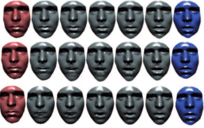
when represented as elements ofSn_{. Shown in Fig. 9}

are examples of some geodesic paths between source and target faces. The three top rows illustrate paths between faces of different subjects, and are termed

inter-class geodesics whereas the remaining rows

illus-trate paths between faces of the same person convey-ing different expressions, and are termed intra-class

geodesics.

These geodesics provide a tangible benefit, beyond the current algorithms that provide some kind of a similarity score for analyzing faces. In addition to their interpretation as optimal deformations under the chosen metric, the geodesics can also be used for computing the mean shape and measuring the shape covariance of a set of faces, as illustrated later. To demonstrate the quality of this deformation, we com-pare it qualitatively for faces with the deformation obtained using a linear interpolation between regis-tered points under an ICP registration of points, in Fig. 10. The three rows show, respectively, a geodesic path in the shape space, the corresponding path in the pre-shape space, and a path using ICP. Algorithm 1

Fig. 9. Examples of geodesics in the shape space. The top three rows illustrate examples of inter-class geodesics and the bottom three rows illustrate intra-class geodesics.

Fig. 10. Examples of geodesics in shape space (top row), pre-shape space (middle row) and a linearly interpolated path after ICP alignment (bottom row).

is used to calculate the geodesic path in the shape space. In other words, the optimal matching (re-parameterization) between curves is established and, thus, anatomical points well matched across the two surfaces. The upper lips match the upper lips, for instance, and this helps produce a natural opening of the mouth as illustrated in the top row in Fig. 10. However, the optimal matching is not established yet when the geodesic is calculated in the pre-shape space. This results in an unnatural deformation along the geodesic in the mouth area.

Fig. 11. Karcher mean of eight faces (left) is shown on the right.

3.3 Computation of the Mean Shape

As mentioned above, an important advantage of our Riemannian approach over many past papers is its ability to compute summary statistics of a set of faces. For example, one can use the notion of Karcher mean [14] to define an average face that can serve as a representative face of a group of faces. To calculate

a Karcher mean of facial surfaces {S1_{, ..., S}k_{} in S}n_,

we define an objective function:V : Sn _{→ R, V(S) =}

Pk

i=1dS(Si, S)2. The Karcher mean is then defined by:

S = arg minS∈SnV(S). The algorithm for computing

Karcher mean is a standard one, see e.g. [8], and is not repeated here to save space. This minimizer may not be unique and, in practice, one can pick any one of those solutions as the mean face. This mean has a nice geometrical interpretation: S is an element of

Sn _{that has the smallest total (squared) deformation}

from all given facial surfaces{S1_{, ..., S}k_{}. An example}

of a Karcher mean face for eight faces belonging to different people is shown in Fig. 11.

3.4 Completion of Partially-Obscured Curves

Earlier we have introduced a filtering step that finds and removes curves with missing parts. Although this step is effective in handling some missing parts, it may not be sufficient when parts of a face are missing due to external occlusions, such as glasses and hair. In the case of external occlusions, the majority of radial curves could have hidden parts that should be predicted before using these curves. This prob-lem is more challenging than self-occlusion because, in addition to the missing parts, we can also have parts of the occluding object(s) in the scan. In a non-cooperative situation, where the acquisition is uncon-strained, there is a high probability for this kind of occlusion to occur. Once we detect points that belong to the face and points that belong to the occluding object, we first remove the occluding object and use a statistical model in the shape space of radial curves to complete the broken curves. This replaces the parts of face that have been occluded using information from the visible part and the training data.

The core of this problem, in our representation of facial surfaces by curves, is to take a partial facial curve and predict its completion. The sources of infor-mation available for this prediction are: (1) the current

(partially observed) curve and (2) several (complete) training curves at the same angle that are extracted from full faces. The basic idea is to develop a sparse model for the curve from the training curves and use that to complete the observed curve. To keep the model simple, we use the PCA of the training data, in an appropriate vector space, to form an orthogonal basis representing training shapes. Then, this basis is used to estimate the coefficients of the observed curve and the coefficients help reconstruct the full

curve. Since the shape space of curveS is a nonlinear

space, we use the tangent space Tµ(S), where µ is the

mean of the training shapes, to perform PCA. Let α denote the angular index of the observed curve, and

let qα1, qα2, . . . , qkα be the SRVFs of the curves taken

from the training faces at that angle. As described earlier, we can compute the sample Karcher mean of

their shapes {[qi

α] ∈ S}, denoted by µα. Then, using

the geometry ofS we can map these training shapes in

the tangent space using the inverse exponential map.

We obtain vi,α= exp−1µα(q

i α), where exp−1q1 (q2) = θ sin(θ)(q ∗ 2−cos(θ)q1), θ = cos−1(hq1, q∗2i) , and where q∗

2 is the optimal rotation and

re-parameterization of q2 to be aligned with q1, as

dis-cussed earlier. A PCA of the tangent vectors{vi} leads

to the principal basis vectors u1,α, u2,α, ..., uJ,α, where

J represents the number of significant basis elements.

Now returning to the problem of completing a partially-occluded curve, let us assume that this curve

is observed for parameter value t in [0, τ ]⊂ [0, 1]. In

other words, the SRVF of this curve q(t) is known

for t ∈ [0, τ] and unknown for t > τ. Then, we can

estimate the coefficients of q under the chosen basis

according to cj,α= hq, uj,αi ≈

Rτ

0 hq(t), uj,α(t)i dt, and

estimate the SRVF of the full curve according to ˆ qα(t) = J X j=1 cj,αuj,α(t) , t ∈ [0, 1] .

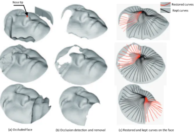
We present three examples of this procedure in Fig. 12, with each face corrupted by an external occlusion as shown in column (a). The detection and removal of occluded parts is performed as described in the previous section, and the result of that step is shown in column (b). Finally, the curves passing through the missing parts are restored and shown in (c).

In order to evaluate this reconstruction step, we have compared the restored surface (shown in the top row of Fig. 12) with the complete neutral face of that class, as shown in Fig. 13. The small values of both absolute deviation and signed deviation, between the restored face and the corresponding face in the gallery, demonstrate the success of the restoration process.

In the remainder of this paper, we will apply this comprehensive framework for 3D face recognition us-ing a variety of well known and challengus-ing datasets.

Restored curves Kept curves

(a) Occluded face (b) Occlusion detec!on and removal (c) Restored and kept curves on the face Nose !p

Fig. 12. (a) Faces with external occlusion, (b) faces after the detection and removal of occluding parts and (c) the estimation of the occluded parts using a statistical model on the shape spaces of curves.

Neutral face

(Gallery) Restored face Alignment

Signed deviaon color map and distribuon between restored face and gallery face Face a!er

occlusion removal

Restoraon

Absolute deviaon color map and distribuon between restored face and gallery face Mesh

generaon Face a!er curves restoraon

Fig. 13. Illustration of a face with missing data (after occlusion removal) and its restoration. The deviation between the restored face and the corresponding neu-tral face is also illustrated.

These databases have different characteristics and challenges, and together they facilitate an exhaustive evaluation of a 3D face recognition method.

4

E

In the following we provide a comparative perfor-mance analysis of our method with other state-of-the-art solutions, using three datasets: the FRGC v2.0 dataset, the GavabDB, and the Bosphorus dataset.

4.1 Data Preprocessing

Since the raw data contains a number of imperfec-tions, such as holes, spikes, and include some unde-sired parts, such as clothes, neck, ears and hair, the data pre-processing step is very important and non-trivial. As illustrated in Fig. 14, this step includes the following items:

• The hole-filling filter identifies and fills holes in

in-put meshes. The holes are created either because of the absorption of laser in dark areas, such as eyebrows and mustaches, or self-occlusion or

Acquision

before a er

before a er

Filling holes Cropping Smoothing

Result of previous stage Links between stages

Fig. 14. The different steps of preprocessing: acquisi-tion, filling holes, cropping and smoothing

open mouths. They are identified in the input mesh by locating boundary edges, linking them together into loops, and then triangulating the resulting loops.

• A cropping filter cuts and returns parts of the

mesh inside an Euclidean sphere of radius 75mm centered at the nose tip, in order to discard as much hair as possible. The nose tip is automat-ically detected for frontal scans and manually annotated for scans with occlusions and large pose variation.

• A smoothing filter reduces high frequency

compo-nents (spikes) in the mesh, improves the shapes of cells, and evenly distributes the vertices on a facial mesh.

We have used functions provided in the VTK (www.vtk.org) library to develop these filters.

4.2 Comparative Evaluation on the FRGCv2

Dataset

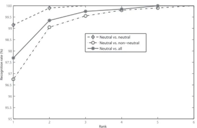
For the first evaluation we use the FRGCv2 dataset in which the scans have been manually clustered into three categories: neutral expression, small expres-sion, and large expression. The gallery consists of the first scans for each subject in the database, and the remaining scans make up the probe faces. This dataset was automatically preprocessed as described in the Section 4.1. Fig. 15 shows Cumulative Matching Curves (CMCs) of our method under this protocol for the three cases: neutral vs. neutral, neutral vs. non-neutral and non-neutral vs. all. Note that this method results in 97.7% rank-1 recognition rate in the case of neutral vs. all. In the difficult scenario of neutral vs. expressions, the rank-1 recognition rate is 96.8%, which represents a high performance, while in the simpler case of neutral vs. neutral the rate is 99.2%.

A comparison of recognition performance of our method with several state-of-the-art results is pre-sented in Table 1. This time, in order to keep the comparisons fair, we kept all the 466 scans in the gallery. Notice that our method achieved a 97% rank-1 recognition which is close to the highest published results on this dataset [29], [26], [9]. Since the scans

1 2 3 4 5 6 95 95.5 96 96.5 97 97.5 98 98.5 99 99.5 100 Rank Recognition rate (% ) Neutral vs. neutral Neutral vs. non−neutral Neutral vs. all

Fig. 15. The CMC curves of our approach for the

following scenario: neutral vs. neutral, neutral vs. ex-pressions and neutral vs. all.

in FRGCv2 are all frontal, the ability of region-based algorithms, such as [9], [26], to deal with the missing parts is not tested in this dataset. For that end, one would need a systematic evaluation on a dataset with the missing data issues, e.g. the GavabDB. The best recognition score on FRGCv2 is reported by Spreeuw-ers [29] which uses an intrinsic coordinate system based on the vertical symmetry plane through the nose. The missing data due to pose variation and occlusion challenges will be a challenge there as well. In order to evaluate the performance of the pro-posed approach in the verification scenario, the Re-ceiver Operating Characteristic (ROC) curves for the ROC III mask of FRGCv2 and ”all-versus-all” are plotted in Fig. 16. For comparison, Table 2 shows the verification results at false acceptance rate (FAR) of 0.1 percent for several methods. For the standard protocol testings, the ROC III mask of FRGC v2, we obtain the verification rates of around 97%, which is comparable to the best published results. In the all-versus-all experiment, our method provides 93.96% VR at 0.1% FAR, which is among the best rates in the table [26], [29], [32]. Note that these approaches are applied to FRGCv2 only. Since scans in FRGCv2 are mostly frontal and have high quality, many methods are able to provide good performance. It is, thus, important to evaluate a method in other situations where the data quality is not as good. In the next two sections, we will consider those situations with the GavabDB involving the pose variation and the Bosphorus dataset involving the occlusion challenge.

4.3 Evaluation on the GavabDB Dataset

Since GavabDB [21] has many noisy 3D face scans un-der large facial expressions, we will use that database to help evaluate our framework. This database con-sists of the Minolta Vi-700 laser range scans from 61 subjects – 45 male and 16 female – all of them Caucasian. Each subject was scanned nine times from different angles and under different facial expressions

TABLE 1

Comparison of rank-1 scores on the FRGCv2 dataset with the state-of-the-art results.

Spreeuwers [29] Wang et al. [32] Haar et al. [31] Berretti et al. [2] Queirolo et al. [26] Faltemier et al. [9] Kakadiaris et al. [13] Our approach

99% 98.3% 97% 94.1% 98.4% 97.2% 97% 97%

TABLE 2

Comparison of verification rates at FAR=0.1% on the FRGCv2 dataset with state-of-the-art results (the ROC III mask and the All vs. All scenario).

Approaches Kakadiaris et al. [13] Faltemier et al. [9] Berretti et al. [2] Queirolo et al. [26] Spreeuwers [29] Wang et al. [32] Our approach

ROC III 97% 94.8% - 96.6% 94.6% 98.4% 97.14% All vs. All - 93.2% 81.2% 96.5% 94.6% 98.13% 93.96% 10−1 100 101 102 89 90 91 92 93 94 95 96 97 98 99 100 FAR (%) VR (%) All vs All ROC III

Fig. 16. The ROC curves of our approach for the

following scenario: All vs. All and the ROC III mask.

(six with the neutral expression and three with non-neutral expressions). The non-neutral scans include sev-eral frontal scans – one scan while looking up (+35 degree), one scan while looking down (-35 degree), one scan from the right side (+90 degree), and one from the left side (-90 degree). The non-neutral scans include cases of a smile, a laugh, and an arbitrary expression chosen freely by the subject. We point out that in these experiments the nose tips in profile faces have been annotated manually.

One of the two frontal scans with the neutral ex-pression for each person is taken as a gallery model, and the remaining are used as probes. Table 3 com-pares the results of our method with the previously published results following the same protocol. As noted, our approach provides the highest recognition rate for faces with non-neutral expressions (94.54%). This robustness comes from the use of radial, elastic curves since: (1) each curve represents a feature that characterizes local geometry and, (2) the elastic match-ing is able to establish a correspondence with the correct alignment of anatomical facial features across curves.

Fig. 17 illustrates examples of correct and incorrect matches for some probe faces. In each case we show a pair of faces with the probe shown on the left and the top ranked gallery face shown on the right. These

pic-tures also exhibit examples of the variability in facial expressions of the scans included in the probe dataset. As far as faces with the neutral expressions are con-cerned, the recognition accuracy naturally depends on their pose. The performance decreases for scans from the left or right sides because more parts are occluded in those scans. However, for pose variations up to 35 degrees the performance is still high (100% for looking up and 98.36% for looking down). Fig. 17 (top row) shows examples of successful matches for up and down looking faces and unsuccessful matches for sideways scans.

Fig. 17. Examples of correct (top row) and incorrect matches (bottom row). For each pair, the probe (on the left) and the ranked-first face from the gallery (on the right) are reported.

Table 3 provides an exhaustive summary of results obtained using GavabDB; our method outperforms the majority of other approaches in terms of the recognition rate. Note that there is no prior result in the literature on 3D face recognition using sideway-scans from this database. Although our method works well on common faces with a range of pose variations within 35 degrees, it can potentially fail when a large part of the nose is missing, as it can cause an incorrect alignment between the probe and the gallery. This situation occurs if the face is partially occluded by external objects such as glasses, hair, etc. To solve this problem, we first restore the data missing due to occlusion.

4.4 3D Face Recognition on the Bosphorus

Dataset: Recognition Under External Occlusion

In this section we will use components I (occlusion detection and removal) and II (missing data

restora-TABLE 3

Recognition results comparison of the different methods on the GavabDB.

Lee et al. [16] Moreno et al. [22] Mahoor et al. [18] Haar et al. [31] Mousavi et al. [23] Our method

Neutral 96.67% 90.16% - - - 100%

Expressive 93.33% 77.9% 72% - - 94.54%

Neutral+expressive 94.68% - 78% - 91% 95.9%

Rotated looking down - - 85.3% - - 100%

Rotated looking up - - 88.6% - - 98.36%

Overall - - - 98% 81.67% 96.99%

Scans from right side - - - 70.49%

Scans from left side - - - 86.89%

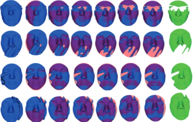
tion) in the algorithm. The first problem we encounter in externally-occluded faces is the detection of the external object parts. We accomplish this by com-paring the given scan with a template scan, where a template scan is developed using an average of training scans that are complete, frontal and have neutral expressions. The basic matching procedure between a template and a given scan is recursive ICP, which is implemented as follows. In each iteration, we match the current face scan with the template using ICP and remove those points on the scan that are more than a certain threshold away from the corresponding points on the template. This threshold has been determined using experimentation and is fixed for all faces. In each iteration, additional points that are considered extraneous are incrementally re-moved and the alignment (with the template) based on the remaining points is further refined. Fig. 18 shows an example of this implementation. From left to right, each face shows an increasing alignment of the test face with the template, with the aligned parts shown in magenta, and also an increasing set of points labeled as extraneous, drawn in pink. The final result, the original scan minus the extraneous parts, is shown in green at the end.

Fig. 18. Gradual removal of occluding parts in a face scan using Recursive-ICP.

In the case of faces with external occlusion, we first restore them and then apply the recognition procedure. That is, we detect and remove the oc-cluded part, and recover the missing part resulting in a full face that can be compared with a gallery

face using the metric dS. The recovery is performed

using the tangent PCA analysis and Gaussian models, as described in Section 3.4. In order to evaluate our approach, we perform this automatic procedure on the Bosphorus database [1]. We point out that for this dataset the nose tip coordinates are already provided. The Bosphorus database is suitable for this evaluation as it contains scans of 60 men and 45 women, 105 subjects in total, in various poses, expressions and in the presence of external occlusions (eyeglasses, hand, hair). The majority of the subjects are aged between 25 and 35. The number of total face scans is 4652; at least 54 scans each are available for most of the subjects, while there are only 31 scans each for 34 of them. The interesting part is that for each subject there are four scans with occluded parts. These occlusions refer to (i) mouth occlusion by hand, (ii) eyeglasses, (iii) occlusion of the face with hair, and (iv) occlusion of the left eye and forehead regions by hands. Fig. 19 shows sample images from the Bosphorus 3D database illustrating a full scan on the left and the remaining scans with typical occlusions.

Fig. 19. Examples of faces from the Bosphorus

database. The unoccluded face on the left and the different types of occlusions are illustrated.

We pursued the same evaluation protocol used in the previously published papers: a neutral scan for each person is taken to form a gallery dataset of size 105 and the probe set contains 381 scans that have occlusions. The training is performed using other sessions so that the training and test data are disjoint. The rank-1 recognition rate is reported in Fig. 20 for different approaches depending upon the type of occlusion. As these results show the process of restoring occluded parts significantly increases the accuracy of recognition. The rank-1 recognition rate is 78.63% when we remove the occluded parts and apply the recognition algorithm using the remaining parts, as described in Section 2.4. However, if we

Restored curves Kept curves

Fig. 21. Examples of non recognized faces. Each row illustrates, from left to right, the occluded face, the result of occlusion removal and the result of restoration.

perform restoration, the recognition rate is improved to 87.06%. Clearly, this improvement in performance is due to the estimation of missing parts on curves. These parts, that include important shape data, were not considered by the algorithm described earlier. Even if the part added with restoration introduces some error, it still allows us to use the shapes of the partially observed curves. Furthermore, during restoration, the shape of the partially observed curve is conserved as much as possible.

Examples of 3D faces recognized by our approach are shown in Fig. 12, along with different steps of the algorithm. The faces in the two bottom rows are exam-ples of incorrectly recognized faces by our algorithm without restoration (as described earlier), but after the restoration step, they are correctly recognized. Aluz et al [1] reported a 93.69% rank-1 recognition rate overall for this database using the same protocol that we have described above. While this reported perfor-mance is very good, their processing has some manual components. Actually, the authors partition the face manually and fuse the scores for matching different parts of the face together. In order to compare with Colombo et al. [6], we reduce the probe dataset to 360 by discarding bad quality scans as Colombo et al. [6] did. Our method outperforms their approach with an overall performance of 89.25%, although individually our performance is worse in the case of occlusion by hair. It is difficult, in this case, to completely overcome face occlusion. Therefore, during the restoration step, our algorithm tries to keep majority of parts. This leads to a deformation in the shape of curves and, hence, affects the recognition accuracy. We present some examples of unrecognized faces in the case of occlusion by hair in Fig. 21. In this instance, the removal of curves passing through occlusion is better than restoring them as illustrated in Fig. 20.

5

D

In order to study the performance of the proposed approach in presence of different challenges, we have presented experimental results using three well-known 3D face databases. We have obtained

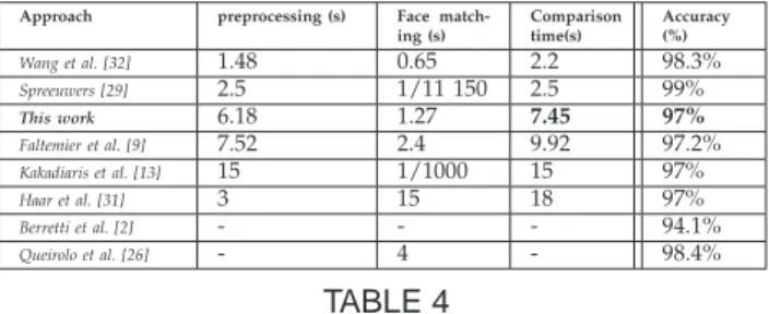
com-Approach preprocessing (s) Face

match-ing (s) Comparison time(s) Accuracy (%) Wang et al. [32] 1.48 0.65 2.2 98.3% Spreeuwers [29] 2.5 1/11 150 2.5 99% This work _{6.18 1.27} 7.45 97% Faltemier et al. [9] 7.52 2.4 9.92 97.2% Kakadiaris et al. [13] 15 1/1000 15 97% Haar et al. [31] 3 15 18 97% Berretti et al. [2] - - - 94.1% Queirolo et al. [26] - 4 - 98.4% TABLE 4

Comparative study of time implementations and recognition accuracy on FRGCv2 of the proposed

approach with state-of-the-art.

petitive results relative to the state of the art for 3D face recognition in presence of large expressions, non-frontal views and occlusions. As listed in Table 4, our fully automatic results obtained on the FRGCv2 are near the top. Table 4 also reports the computa-tional time of our approach and some state of the art methods on the FRGCv2 dataset. For each ap-proach, we report the time needed for preprocessing and/or feature extraction in the first column. In the second column we report the time needed to compare two faces. The third column is the sum of the two previous computation times for each approach. In the last column, we report the accuracy (recognition rate on FRGCv2) of different approaches. Regarding computational efficiency, parallel techniques can also be exploited to improve performance of our approach since the computation of curve distances, preprocess-ing, etc, are independent tasks.

In the case of GavabDB and Bosphorus, the nose tip was manually annotated for non frontal and occluded faces. In the future, we hope to develop automatic nose tip detection methods for non frontal views and for faces that have undergone occlusion.

6

C

In this paper we have presented a framework for a sta-tistical shape analysis of facial surfaces. We have also presented results on 3D face recognition designed to handle variations of facial expression, pose variations and occlusions between gallery and probe scans. This method has several properties that make it appropri-ate for 3D face recognition in non-cooperative scenar-ios. Firstly, to handle pose variation and missing data, we have proposed a local representation by using a curve representation of a 3D face and a quality filter for selecting curves. Secondly, to handle variations in facial expressions, we have proposed an elastic shape analysis of 3D faces. Lastly, in the presence of occlusion, we have proposed to remove the occluded parts then to recover only the missing data on the 3D scan using statistical shape models. That is, we have constructed a low dimensional shape subspace for each element of the indexed collection of curves,

Eye Mouth Glasses Hair All occlusions 60 65 70 75 80 85 90 95 100 105

Rank−1 recognition Rate (%

)

Our approach (all scans) Colombo et al. [6] (360 scans) Our approach (360 scans) Occlusion removal only (all scans) Aluz et al. [1] (all scans) 93.6% 86.6% 98.9% 91.1% 93.6% 97.1% 65.7% 78% 78.5% 74.7% 97.8% 81% 94.2% 89.6% 90.4% 78.7% 85.2% 81% 93.6% 78.6% 89.2% 87.6% 87%

Fig. 20. Recognition results on the Bosphorus database and comparison with state-of-the-art approaches.

and then represent a curve (with missing data) as a linear combination of its basis elements.

A

This work was supported by the French research agency ANR through the 3D Face Analyzer project under the contract ANR 2010 INTB 0301 01 and the project FAR3D ANR-07-SESU-04. It was also partially supported by ”NSF DMS 0915003” and ”NSF DMS 1208959” grants to Anuj Srivastava.

R

[1] N. Alyuz, B. Gokberk, and L. Akarun. A 3D face recognition

system for expression and occlusion invariance. In Biometrics:

Theory, Applications and Systems, 2008. BTAS 2008. 2nd IEEE International Conference on, 29 2008.

[2] S. Berretti, A. Del Bimbo, and P. Pala. 3D face recognition using

isogeodesic stripes. IEEE Transactions on Pattern Analysis and

Machine Intelligence, 32(12):2162–2177, 2010.

[3] K. W. Bowyer, K. Chang, and P. Flynn. A survey of approaches

and challenges in 3D and multi-modal 3D + 2D face recogni-tion. Comput. Vis. Image Underst., 101(1):1–15, 2006.

[4] A. M. Bronstein, M. M. Bronstein, and R. Kimmel.

Three-dimensional face recognition. International Journal of Computer

Vision, 64(1):5–30, 2005.

[5] A. M. Bronstein, M. M. Bronstein, and R. Kimmel.

Expression-invariant representations of faces. IEEE Transactions on Image

Processing, 16(1):188–197, 2007.

[6] A. Colombo, C. Cusano, and R. Schettini. Three-dimensional

occlusion detection and restoration of partially occluded faces.

Journal of Mathematical Imaging and Vision, 40(1):105–119, 2011.

[7] H. Drira, B. Ben Amor, M. Daoudi, and A. Srivastava. Pose

and expression-invariant 3D face recognition using elastic

radial curves. In Proceedings of the British Machine Vision

Conference, pages 1–11. BMVA Press, 2010. doi:10.5244/C.24.90.

[8] H. Drira, B. Ben Amor, A. Srivastava, and M. Daoudi. A

Riemannian analysis of 3D nose shapes for partial human biometrics. In IEEE International Conference on Computer Vision, pages 2050–2057, 2009.

[9] T. C. Faltemier, K. W. Bowyer, and P. J. Flynn. A region

en-semble for 3D face recognition. IEEE Transactions on Information

Forensics and Security, 3(1):62–73, 2008.

[10] G. Gordan. Face recognition based on depth and curvature features. In Proceedings of Conference on Computer Vision and

Pattern Recognition, CVPR, pages 108–110, 1992.

[11] S. Gupta, J. K. Aggarwal, M. K. Markey, and A. C. Bovik. 3D face recognition founded on the structural diversity of human faces. In Proceeding of Computer Vision and Pattern Recognition,

CVPR, 2007.

[12] D. Huang, G. Zhang, M. Ardabilian, Wang, and L. Chen. 3D face recognition using distinctiveness enhanced facial repre-sentations and local feature hybrid matching. In Fourth IEEE

International Conference on Biometrics: Theory Applications and Systems (BTAS), pages 1–7, 2010.

[13] I. A. Kakadiaris, G. Passalis, G. Toderici, M. N. Murtuza, Y. Lu, N. Karampatziakis, and T. Theoharis. Three-dimensional face recognition in the presence of facial expressions: An annotated

deformable model approach. IEEE Transactions on Pattern

Analysis and Machine Intelligence, 29(4):640–649, 2007.

[14] H. Karcher. Riemannian center of mass and mollifier smooth-ing. Communications on Pure and Applied Mathematics, 30:509– 541, 1977.

[15] Y. Lee, H. Song, U. Yang, H. Shin, and K. Sohn. Local feature based 3D face recognition. In Proceedings of Audio- and

Video-Based Biometric Person Authentication, AVBPA, pages 909–918,

2005.

[16] X. Li, T. Jia, and H. Zhang. Expression-insensitive 3D face

recognition using sparse representation. Computer Vision

and Pattern Recognition, IEEE Computer Society Conference on,

0:2575–2582, 2009.

[17] X. Lu and A. Jain. Deformation modeling for robust 3D face matching. IEEE Transactions on Pattern Analysis and Machine

Intelligence, 30(8):1346 –1357, aug. 2008.

[18] M. H. Mahoor and M. Abdel-Mottaleb. Face recognition

based on 3D ridge images obtained from range data. Pattern

Recognition, 42(3):445–451, 2009.

[19] R. McKeon and T. Russ. Employing region ensembles in a statistical learning framework for robust 3D facial recognition. In Fourth IEEE International Conference on Biometrics: Theory

Applications and Systems (BTAS), pages 1–7, 2010.

[20] A. Moorthy, A. Mittal, S. Jahanbin, K. Grauman, and A. Bovik. 3D facial similarity: automatic assessment versus perceptual judgments. In Fourth IEEE International Conference on

Biomet-rics: Theory Applications and Systems (BTAS), pages 1–7, 2010.

[21] A. B. Moreno and A. Sanchez. Gavabdb: A 3D face database. In Workshop on Biometrics on the Internet, pages 77–85, 2004. [22] A. B. Moreno, A. Sanchez, J. F. Velez, and F. J. Daz. Face

recognition using 3D local geometrical features: Pca vs. svm. In Int. Symp. on Image and Signal Processing and Analysis, 2005. [23] M. H. Mousavi, K. Faez, and A. Asghari. Three dimensional face recognition using svm classifier. In ICIS ’08: Proceedings

of the Seventh IEEE/ACIS International Conference on Computer and Information Science, pages 208–213, Washington, DC, USA,

2008.

[24] I. Mpiperis, S. Malassiotis, and M. G. Strintzis. 3D face

recognition with the geodesic polar representation. IEEE

Transactions on Information Forensics and Security, 2(3-2):537–

547, 2007.

[25] G. Passalis, P. Perakis, T. Theoharis, and I. A. Kakadiaris. Using facial symmetry to handle pose variations in real-world 3D face recognition. IEEE Transactions on Pattern Analysis and

Machine Intelligence, 33(10):1938–1951, 2011.

[26] C. C. Queirolo, L. Silva, O. R. Bellon, and M. P. Segundo. 3D face recognition using simulated annealing and the surface

interpenetration measure. IEEE Transactions on Pattern Analysis

and Machine Intelligence, 32:206–219, 2010.

[27] C. Samir, A. Srivastava, and M. Daoudi. Three-dimensional face recognition using shapes of facial curves. IEEE

Transac-tions on Pattern Analysis and Machine Intelligence, 28:1858–1863,

2006.

[28] C. Samir, A. Srivastava, M. Daoudi, and E. Klassen. An

intrinsic framework for analysis of facial surfaces. International

Journal of Computer Vision, 82(1):80–95, 2009.

[29] L. Spreeuwers. Fast and accurate 3D face recognition using registration to an intrinsic coordinate system and fusion of multiple region classifiers. International Journal of Computer

Vision, 93(3):389–414, 2011.

[30] A. Srivastava, E. Klassen, S. H. Joshi, and I. H. Jermyn. Shape analysis of elastic curves in euclidean spaces. IEEE Transactions

on Pattern Analysis and Machine Intelligence, 33(7):1415–1428,

2011.

[31] F. ter Haar and R. C. Velkamp. Expression modeling for

expression-invariant face recognition. Computers and Graphics, 34(3):231–241, 2010.

[32] Y. Wang, J. Liu, and X. Tang. Robust 3D face recognition by local shape difference boosting. IEEE Transactions on Pattern

Analysis and Machine Intelligence, 32:1858–1870, 2010.

[33] L. Younes, P. W. Michor, J. Shah, and D. Mumford. A metric on shape space with explicit geodesics. Rend. Lincei Mat. Appl.

9, 9:25–57, 2008.

Hassen Drira is an assistant

Professor of Computer Science

at Institut Mines-T´el´ecom/T´el´ecom Lille1, LIFL UMR (CNRS 8022) since September 2012. He received

his engineering degree in 2006

and his M.Sc. degrees Computer

Science in 2007 from National

School of Computer Science (ENSI), Manouba, Tunisia. He obtained his Ph.D degree in Computer Science in 2011, from University of Lille 1, France. He spent the year 2011-2012 in the MIIRE research group within the Fundamental Computer Science Laboratory of Lille (LIFL) as a Post-Doc. His research interests are mainly focused on pattern recognition, statistical analysis, 3D face recognition, biometrics and more recently 3D facial expression recognition. He has published several refereed journal and conference articles in these areas.

Boulbaba Ben Amor received the

M.S. degree in 2003 and the Ph.D. degree in Computer Science in 2006, both from Ecole Centrale de Lyon, France. He obtained the engineer degree in computer science from ENIS, Tunisia, in 2002. He jointed the Mines-T´el´ecom/T´el´ecom Lille1 Institute as associate-professor, in 2007. Since then, he is also member of the Computer Science Laboratory in University Lille 1 (LIFL UMR CNRS 8022). His research interests are mainly focused on statistical three-dimensional face analysis and recognition and facial expression recognition using 3D. He is co-author of several papers in refereed journals and proceedings of international conferences. He has been involved in French and

International projects and has served as program committee member and reviewer for international journals and conferences.

Anuj Srivastava is a Professor

of Statistics at the Florida State University in Tallahassee, FL. He obtained his MS and PhD degrees in Electrical Engineering from the Washington University in St. Louis

in 1993 and 1996, respectively.

After spending the year 1996-97 at the Brown University as a visiting researcher, he joined FSU as an Assistant Professor in 1997. His research is focused on pattern theoretic approaches to problems in image analysis, computer vision, and signal processing. Specifically, he has developed

computational tools for performing statistical

inferences on certain nonlinear manifolds and has published over 200 refereed journal and conference articles in these areas.

Mohamed Daoudi is a Professor

of Computer Science at TELECOM Lille 1 and LIFL (UMR CNRS 8022). He is the head of Computer

Science department at T´el´ecom

Lille1. He received his Ph.D. degree

in Computer Engineering from

the University of Lille 1 (USTL), France, in 1993

and Habilitation Diriger des Recherches from the

University of Littoral, France, in 2000. He was the founder and the scientific leader of MIIRE research

group http://www-rech.telecom-lille1.eu/miire/.

His research interests include pattern recognition, image processing, three-dimensional analysis and retrieval and 3D face analysis and recognition. He has published over 100 papers in some of

the most distinguished scientific journals and

international conferences. He is the co-author of the book ”3D processing: Compression, Indexing and Watermarking (Wiley, 2008). He is Senior member IEEE.

Rim Slama received the

engineer-ing and M.Sc. degree in Computer Science from National School of Computer Science (ENSI), Manouba, Tunisia, in 2010 and 2011, respec-tively. Currently she is a Ph.D. can-didate and a member in the MIIRE research group within the Funda-mental Computer Science Laboratory of Lille (LIFL), France. Her current research interests include human motion analysis, computer vision, pattern recognition, 3D video sequences of people, dynamic 3D human body, shape matching and their applications in com-puter vision.