Dynamics of mineral elements under a fast-growing eucalyptus plantation in Brazil. Implications for soil sustainability.

HAL Id: pastel-00610330

https://pastel.archives-ouvertes.fr/pastel-00610330

Submitted on 21 Jul 2011

HAL is a multi-disciplinary open access

archive for the deposit and dissemination of sci-entific research documents, whether they are pub-lished or not. The documents may come from teaching and research institutions in France or abroad, or from public or private research centers.

L’archive ouverte pluridisciplinaire HAL, est destinée au dépôt et à la diffusion de documents scientifiques de niveau recherche, publiés ou non, émanant des établissements d’enseignement et de recherche français ou étrangers, des laboratoires publics ou privés.

eucalyptus plantation in Brazil. Implications for soil

sustainability.

Valérie Maquere

To cite this version:

Valérie Maquere. Dynamics of mineral elements under a fast-growing eucalyptus plantation in Brazil. Implications for soil sustainability.. Silviculture, forestry. AgroParisTech, 2008. English. �NNT : 2008AGPT0086�. �pastel-00610330�

L’Institut des Sciences et Industries du Vivant et de l’Environnement (Agro Paris Tech) est un Grand Etablissement dépendant du Ministère de l’Agriculture et de la Pêche, composé de l’INA PG, de l’ENGREF et de l’ENSIA

(décret n° 2006-1592 du 13 décembre 2006)

N° /__/__/__/__/__/__/__/__/__/__/

P h D T H E S I S

for the degree of

Doctor

of

the Institut des Sciences et Industries du Vivant et de l’Environnement

(Agro Paris Tech)

the Universidade de São Paulo, Escola Superior de Agricultura Luiz de Queiroz

Area: Forest Sciences

by

Valérie MAQUERE

defended on

DYNAMICS OF MINERAL ELEMENTS UNDER A FAST-GROWING

EUCALYPTUS

PLANTATION IN BRAZIL.

IMPLICATIONS FOR SOIL SUSTAINABILITY.

Thesis Diretor Brazil: José Leonardo de Moraes GONCALVES Supervisor: Jean-Paul LACLAU

INRA Unité Biogéochimie des Ecosystèmes Forestiers, Champenoux, France

CIRAD UPR Fonctionnement et pilotage des écosystèmes de plantations, Montpellier, France ESALQ Departamento de Ciências Florestais, Piracicaba, Brasil

Jury:

Mr Bruno Delvaux, Professor, Catholic University of Louvain, Belgium ...Reviewer Mr Alex Vladimir Krushe, Researcher, CENA/USP, Brazil...Reviewer Mr Marc Voltz, Research Director, INRA, France...Reviewer

Mr Bruno Ferry, Lecturer, ENGREF, France ...Examinor Mr Julien Tournebize, Researcher, CEMAGREF, France ...Examinor Mr José Leonardo de Moraes Gonçalves, Professor Doctor, ESALQ/USP, Brazil ...Director Mr Jacques Ranger, Research Director, INRA, France ...Director Mr Jean-Paul Laclau, Researcher, CIRAD/USP, Brazil ...Supervisor

A

L’absent

Ce frère brutal mais dont la parole était sûre, patient au sacrifice, diamant et sanglier, ingénieux et secourable, se tenait au centre de tous les malentendus tel un arbre de résine dans le froid inalliable. Au bestiaire de mensonges qui le tourmentait de ses gobelins et de ses trombes il opposait son dos perdu dans le temps. Il venait à vous par des sentiers invisibles, favorisait l’audace écarlate, ne vous contrariait pas, savait sourire. Comme l’abeille quitte le verger pour le fruit déjà noir, les femmes soutenaient sans le trahir le paradoxe de ce visage qui n’avait pas des traits d’otage.

J’ai essayé de vous decrire ce compère indélébile que nous sommes quelques-uns à avoir fréquenté. Nous dormirons dans l’espérance, nous dormirons en son absence, puisque la raison ne soupçonne pas que ce qu’elle nomme, à la légère, absence, occupe le fourneau dans l’unité.

René Char, Seuls demeurent, 1938-1944

Merci à ceux qui ont été là

A l’occasion d’un geste, d’une amitié partagée ou d’une vie passée

Cette thèse est la vôtre. Saravá !

Many thanks to those who participated in this project: For thesis direction:

Jacques Ranger, José Leonardo de Moraes Gonçalves and Jean-Paul Laclau For institutional supervision:

Bruno Ferry For their scientific advises:

Marie-Pierre Turpault, Frédéric Gérard, Bruno Delvaux

Bénédicte Augeard, Thomas Delfosse, Bernard Longdoz, Jean Pétard For funding:

• French Ministry of Agriculture and Fishing (GREF) (salary) • CIRAD and INRA (thesis funding and technical assistance)

• USP/COFECUB (No. 2003.1.10895.1.3) (experimental project funding) • FAPESP (No. 2002/11827-9) (experimental project funding)

• French Ministry of Foreign Affairs (experimental project funding)

• European Ultra Low CO2 Steelmaking project (ULCOS - Contract n°515960) (experimental project funding)

Main laboratories:

• INRA Unité Biogéochimie des Ecosystèmes Forestiers, France: Director Etienne Dambrine. Pascal Bonnaud and all staff.

• CIRAD UPR Fonctionnement et pilotage des écosystèmes de plantations, France: Coordinator Jean-Pierre Bouillet and all staff.

• ESALQ Departamento de Ciências Florestais, Brasil: Prof. Dr. José Leonardo de Moraes Gonçalves and all staff.

Experimental station

• ESALQ Departamento de Ciências Florestais Estação Experimental de Ciências Florestais de Itatinga, Brasil: Rildo Moreira e Moreira and all staff.

Partner laboratories: Brazil

• CENA Laboratório de Biogeoquímica Ambiental. Carlos C. Cerri Marisa de Cássia Piccolo and all staff.

• CENA Laboratorio de Ecologia Isotópica. Prf Dr Reynaldo L. Victória, Alex Vladimir Krusche and all staff.

• CENA Laboratório de Química Analítica. Prf Dr Maria Fernanda Giné Rosías, Aparecida de Fátima Patreze.

• CENA Laboratório de Tratamento de Resíduos. Glauco Arnold Tavares, Juliana Graciela Giovannini.

• ESALQ Departamento de Ciências Florestais Laboratorio de Ecologia Aplicada. Coordinator Alba Valéria Masetto and all staff.

• ESALQ Departamento de Ciências Florestais Laboratório de Química, Celulose e Energia, Prf Dr Francides Gomes da Silva Júnior.

• ESALQ, Departamento de Ciências do solo, Laboratórios de Análises Químicas – Pesquisa, Coordinator Prof.Dr. Luís Reynaldo F. Alleoni. Luis Antonio Silva Junior.

• ESALQ, Departamento de Ciências do solo, Laboratório de Tecidos Vegetais. Coordinator Prof.Dr. Francisco Antonio Monteiro, Lurdes Aparecida D. Gonzáles. • ESALQ, Departamento de Engenharia Rural, Laboratório de Física de Solos.

Gilmar Batista Grigolon. Partner laboratories: France

• CIRAD Unité Opérationelle Sols et Eaux, Montpellier France. Marc Szwarc. • CRPG/CNRS, Service d'Analyse des Roches et des Minéraux. J. Carignan.

• INRA, Unité mixte de recherche Écologie et écophysiologie forestières. Jacqueline Marchand.

• Université de Poitiers, UMR 6532 HYDRASA. Laurent Caner. Many thanks to all the students who study at night and work at day:

Aline, Claudia, David, Gustavo, Leonardo, Mariana, Robson, Tamara, Tiago, … And to those who shared pit digging experiences in Itatinga:

Selma, Julio, Junior, Marcello, Matthieu, Juan, Eduardo.

Many thanks to the PTSM and to the nursery for sharing their working space with me, and to the Laclau’s family for its warm welcome in Brazil.

A

Each year the area of fast-growing tree plantations in the world expands by around one million hectares and concerns are rising regarding their influence on soil fertility and water resources. A comprehensive approach is currently being conducted at the University of São Paulo to study the biogeochemical cycles of nutrients in Eucalyptus grandis plantations. As part of this study, the present thesis focuses on the interactions between the soil matrix and the soil solutions during the first two years of growth of the stand to (i) identify the determinisms driving the chemistry of the soil solution, (ii) quantify the water and nutrient fluxes leaving the ecosystem by deep drainage and thus rule on the risks of groundwater pollution, and (iii) prepare reactive transport modeling using the MIN3P model already tested at the INRA-BEF laboratory.

It is shown that (i) a large uptake of water by the Eucalyptus trees occurred as soon as six months after planting, the water drainage was thus largely reduced at a depth of 3 m after one year of growth, (ii) almost no nutrient was leached below a depth of 3 m, (iii) large amounts of nutrients were released in the upper soil layers and leached down to a depth of 1 m (65-100 kg ha-1 of N-NO3) following clear cutting and fertilizing,

acidification occurred in the upper soil layers but in these ferralsols, the soil Al reserve and buffering capacity are still large, (iv) part of the fertilizers was taken up by the fast growing Eucalyptus trees without appearing in soil solution, (v) S present in the nitrogen fertilizers increased Ca, Mg and P mobilities, and decreased the H and Al release in soil solution, (vi) large quantities of S were adsorbed on the soil surface constituents where sewage sludge or ammonium sulphate was applied, if this sulphate happens to be desorbed, greater soil acidification is to be expected.

It is suggested that the amount of N brought by the fertilizers after one year of growth can be reduced without altering the productivity of the stand but the study of the organic part of the ecosystem seems essential to rule on this point. Long-term monitoring of the ecosystem is needed to assess changes in nutrient dynamics throughout the stand rotation. Isotopic labelling coupled to reactive transport modelling would be useful tools to help understanding the ecosystem functioning.

T

PARTA PREAMBLE THE EXPERIMENT:SITE CHARACTERISTICS EXPERIMENTAL

DESIGN DYNAMICS OF BIOMASS AND NUTRIENT ACCUMULATION 37

A.1 SITE CHARACTERISTICS 41

A.2 THE EXPERIMENT 41

A.3 TREE DEVELOPMENT OVER THE STUDIED PERIOD 47

A.3.1 Experimental methods 47

A.3.2 Main results obtained before clear felling 51 A.3.3 Growth of the newly planted stand: fertilization experiment 53

PARTB THE SOILS OF THE EXPERIMENT: CHARACTERIZATION, MINERALOGY, AND

SURFACE REACTIVITY 61

INTRODUCTION 63

THEORETICAL REMINDERS ON SURFACE CHARGE 68

B.1 MATERIAL AND METHODS 71

B.1.1 Soil general characteristics 71

B.1.2 Soil mineralogy 74

B.1.3 Surface reactivity 82

B.2 RESULTS AND DISCUSSION 84

B.2.1 General characteristics 84

B.2.2 Soil mineralogy 95

B.2.3 Surface reactivity 109

B.3 GENERAL CONCLUSIONS 114

B.3.1 On soil general features 114

B.3.2 On soil spatial heterogeneity 114

B.3.3 On mineral weathering 114

B.3.4 On the expected soil response to the applied fertilizations 115

PARTC WATER FLUXES 119

INTRODUCTION 121

C.1 MATERIAL AND METHODS 124

C.1.1 MIN3P water balance module 124

C.1.2 General characteristics of the performed simulations 131 C.1.3 Time-dependant inputs of the model: daily maximum evaporation

and transpiration, and daily water inflow at the soil surface 136 C.1.4 Data used to assess the simulations’ efficiency: soil water

monitoring 142 C.1.5 Non time-dependant inputs of the model 143

C.1.6 Simulations 147

C.2 RESULTS AND DISCUSSION 153

C.2.1 Time dependant inputs: inflow at the soil surface, maximum evaporation and maximum transpiration 153

C.2.2 Soil water monitoring 158

C.2.3 Conclusions on the spatial heterogeneity of inputs and validation

data sets used in the model 164

C.2.4 Soil hydraulic parameters 165

C.2.5 Simulations 169

C.2.6 Water fluxes budget 187

C.3 GENERAL DISCUSSION AND CONCLUSIONS 191

C.3.1 On soil hydraulic properties 191 C.3.2 On the validity of the simulations 192 C.3.3 On the evapotranspiration of the Eucalyptus stands and on the

water balance 193

C.3.4 On the validity of the model to compute nutrient fluxes and to perform reactive transport modelling 195

PARTD SOIL SOLUTIONS 197

INTRODUCTION 199

D.1 MATERIAL AND METHODS 203

D.1.1 Available data 203

D.1.2 Data analysis 207

D.2 RESULTS AND DISCUSSION 217

D.2.1 Water fluxes collected by the lysimeters calculated from the

MIN3P simulations 217

D.2.2 Median and quartile, aboveground solutions 220 D.2.3 Soil solutions, case study 1: nitrate 225 D.2.4 Soil solutions, case study 2: sulphate 235 D.2.5 Joint dynamics of the measured mineral elements 245

D.3 CONCLUSIONS 263

D.3.1 On the dynamics of nutrients in soils 263

D.3.2 On the methods used 264

PARTE NUTRIENT BUDGETS 267

INTRODUCTION 269

E.1 MATERIAL AND METHODS 271

E.2 RESULTS AND DISCUSSION 279

E.2.1 Nutrient fluxes entering and leaving the studied system 279 E.2.2 Soil water extracts composition at 2 years after planting 283 E.2.3 Changes in adsorbed nutrients from the clear-felling until two

years after planting 287

E.2.4 Global budgets 292

E.3 CONCLUSIONS 297

E.3.1 On the use of fertilizers 297

E.3.2 On the sustainability of the plantation regarding soils and waters 298

E.3.3 On the method used 301

GENERAL CONCLUSIONS AND PERSPECTIVES 303

ANNEXES 307

ANNEX1 TOTAL ANALYSIS OF THE FERTILIZERS APPLIED 309

ANNEX2 COMPLEMENTS TO STAND GROWTH DATA AND DECOMPOSITION RATES

OVER THE EXPERIMENTAL PERIOD 311

ANNEX3 DATA SETS SOILBCF AND SOILAP11: SOIL CHEMICAL AND PHYSICAL

CARACTERISTICS 315

ANNEX4 ABOVEGROUND SOLUTIONS MONITORING 319

ANNEX5 LINEAR REGRESSIONS AMONG THE MEASURED SOIL MOISTURES 331

ANNEX6 SIMULATED AGAINST MEASURED WATER CONTENTS FOR THE BCF AND

CFP PERIODS 333

ANNEX7 CUMULATIVE FLUXES FROM CLEAR FELLING UNTIL THE END OF THE

EXPERIMENTAL PERIOD 335

ANNEX8 SPECIFIC EXTRACTIONS PERFORMED ON SOILS AT AGE 2 YEARS AFTER

PLANTING 337

ARTICLE 341

F

Figure 1 Processes of nutrient transfers occurring within forest ecosystems. ...33 Figure 2 Schematic mass budgets for different sub-systems as part of the ecosystem:

system “tree+ forest floor+soil+soil solution” (A), system “tree” (B), system “forest floor+soil+soil solutions” (C), system “forest floor solutions and soil solutions” (D). Fluxes entering or leaving each system are represented in red arrows. The thesis focuses on the dynamics of system D. Mass budgets were performed for system A. Systems A and C are equivalent once the root uptake is calculated as the sum of litterfall plus nutrient accumulation in trees...36

Figure 3 Localization of the experimental station of Itatinga (São Paulo state,

Brazil) where the fertilization experiment was established...39

Figure 4 Schematic map of each plot of treatments 1, 3 and 5 in blocks 1, 2 and 3

(10 x 10 trees per plot but growth measurements performed on 6 x 6 trees per plot)...42

Figure 5 Experimental design. ...43

Figure 6 Chronology of the experiment...44 Figure 7 Stand vegetal cover over the experimental period: E saligna stand at age

6.5 years before clear felling (BCF period) (A); the stand after it was clear felled (CFP period) (B); the E. grandis seedling fertilized by mineral fertilizers buried at its stem in T1 and T3 (1) or by sewage slugde spread on the forest floor (2) (C); the E. grandis stand at age 6 months (D) and at age 18 months (E) (AP period)...48

Figure 8 E. saligna stand BCF: average and standard deviation of the circumference

at breast height (CBH) of the trees located in the area of the fertilization experiment to be installed after clear felling. ...51

Figure 9 E. saligna stand BCF: coarse and medium roots down to a depth of 3 m.

The average and standard deviation are represented (n=4). ...52

Figure 10 Fine root density (diameter < 1 mm) at the end of the stand rotation (E.

saligna stand BCF) and 12 and 24 months after planting (AP) in treatments 1, 3 and 5.

The average and standard deviations are given (BCF: n=24; AP: n=12)...52

Figure 11 E. grandis stand (AP): average tree height in each treatment as a

percentage of tree height in the control treatment (T1) Significant differences among treatments at levels of 5%, 1%, 0.1% and 0.01% are indicated by *, **, ***, and ****, respectively. NS indicates non significant differences at 5%...54

Figure 12 E. grandis stand (AP): time course of foliar biomass (A) and aboveground

biomass (B) in treatments 1, 3 and 5. Different letters indicate significant differences at P<0.05. ...55

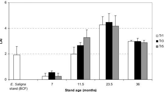
Figure 13 Time course of leaf area index (LAI) before clear felling and after planting

in treatments 1, 3 and 5. Mean and standard deviations (n=4) are represented. ...55

Figure 14 Sampled locations for data set SOILBCF-2 and calculation of a factor f

relating a sample to its distance to the nearest trees. The subscript j (1≤j≤9) and the letter M identify the samples. The subscript i (1≤i≤4) and the letter A identify the nearest trees. ...71

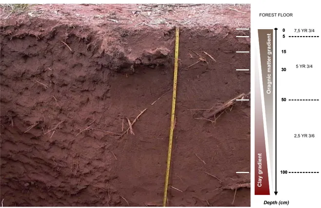
Figure 15 Description of the soil pit excavated in 2003 in the 7-year old Eucalyptus

stand before clear felling. The colour of the different soil layers are given on the right of the depth axis according to Munsell chart...84

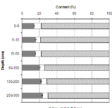
Figure 16 Particle-size distribution performed in hexametaphosphate (da Silva et al.,

1999) for each layer of the soils of the experiment (2003 sampling, data set SOILBCF

-1). Standard errors are represented for the clay fraction (n=9). Sand fraction from 50 µm to 2 mm, silt fraction from 2 to 50 µm and clay fraction < 2 µm. ...86

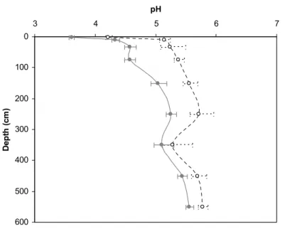
Figure 17 pH measured in water and in KCl 1 mol L-1 for each soil layer in the

experiment (2003 sampling, data sets SOILBCF-1 & 2). Standard errors calculated from

H+ concentrations are represented (n=36 for the 0-5 cm layer, n=9 otherwise)...87

Figure 18 Effective CEC (Rouiller et al., 1980) and saturation in alkaline earths

cations for each layer of the soils of the experiment (2003 sampling, data sets SOILBCF-1 & 2). Standard errors are represented (n=36 for the 0-5 cm layer, n=9

otherwise). ...88

Figure 19 Cation exchange capacity (CEC in cmolc kg-1) (A) and sand content (%)

(B) as a function of the organic carbon (C) content (%) for data sets SOILBCF-1a and

SOILBCF-1b. The measured data and the corresponding linear regressions from Table

13 are represented...91

Figure 20 Linear regression of organic carbon C (%) as a function of the distance to

the nearest trees (f coefficient of Figure 14) calculated for data set SOILBCF-2. f=0

corresponds to a maximum influence of the trees, and f=1 to a minimum influence of the trees. R-square, F value and P>F, together with the intercept and slope calculated for the regression are given (n=27). ...93

Figure 21 Particle-size analysis performed in hexametaphosphate (HMP) and in

water for pit 3 of data set SOILAP11. Standard errors of the analytical repetitions are

given for clay and sand fractions when n≥3. ...95

Figure 22 Mineralogy of the clay and sand fractions: XR diffractograms performed

on oriented deposit of the clay fraction Mg2+ saturated and on raw powder of the sand fraction for block 3, layer 5-15 cm of data set SOILAP11. The main peaks are given in

nm together with the mineral they identify. ...99

Figure 23 Homogeneity with depth of the mineralogy of the clay fraction: RX

diffractograms performed on raw powder of the clay fraction Mg2+ saturated for block 3 of data set SOILAP11, layers 0-5 cm and 200-300 cm. The main peaks are given in nm

together with the mineral they identify. ...100

Figure 24 Spatial homogeneity of the mineralogy of the clay fraction: RX

diffractograms performed on oriented deposit of the clay fraction Mg2+ saturated for all blocks of data set SOILAP11, layer 0-5 cm. The main peaks are given in nm together

with the mineral they identify...101

Figure 25 Identification of the peak at 1.431 nm: influence of treatments (Mg2+

saturation, ethylene glycol (EG) treatment, DCB followed by tricitrate extractions and saturation by K+, heating at 550°C) on RX diffractograms performed on oriented deposits of the clay fraction for layer 5-15 cm block 3 of data set SOILAP11...102

Figure 26 Al2O3 extracted (%) by different analytical methods (oxalate, DCB and

tricitrate) from the clay fraction of pit 3 of data set SOILAP11. Al2O3 from gibbsite and

Figure 27 Estimated mineralogical composition of the bulk soil calculated from

§ B.1.2.6.4 for pit 3 of data set SOILAP11. ...105

Figure 28 Change in cation exchange capacity (CEC), basic cation exchange capacity

(CECb) and anion exchange capacity (AEC) with pH and depth for pit 3 of data set

SOILAP11. The pH for which AEC equals CEC (point of zero net charge pH0) together

with the pH in CaCl2 0.002 mol L-1, in KCl 1 mol L-1 and in water are also given. ...110

Figure 29 Isotherms of adsorption measured for the 0-5 cm layer (A) and the 200-300

cm layer (B) for nitrate, sulphate and phosphate. The Langmuir and Freundlich equations fitted on experimental data are represented. The grey zone on the graphics corresponds to the equivalent AEC (values of Table 20) for N-NO3-, S-SO42-, and

H-H2PO4-. ...112

Figure 30 Influence of the transpiration parameters on the transpiration reduction

factor Rtransp (eq (43)). Rtransp can be expressed as a function of the reserve of

extractable water (REW) or as a function of the saturation in water Sa (eq (44)). Sa is

controlled by ψf, the pressure head below which Rtransp≤1, and by ψlim, the pressure

head below which the transpiration stops (fixed at -150 m in the figure). The curve shape is controlled by REW0 and p1 (eq (43)). ...129

Figure 31 Aboveground water fluxes collectors: stemflow (A); throughfall (B) and

surface run-off (C)...140

Figure 32 Interval drainage experiment (a) during pounding (b) during transient

drainage (the plastic sheet ensures a zero-flux top boundary)...144

Figure 33 Time course of the RF factor (eq. (55) & (56)) reducing the maximum

transpiration (Tmax) over the AP period. The corresponding Tmax for the BCF and the

AP periods are given...151

Figure 34 Time course of temperature, rainfall and evapotranspiration (ET) over the

time of the experiment. The rainfall partition between stemflow, throughfall and interception is given. From 02/2004 to 02/2005, interception represents rainfall since throughfall was not monitored during this period (young Eucalyptus trees). The maximum evapotranspiration (ETmax) and the FAO reference evapotranspiration

(ETref) are given...154

Figure 35 Root length density measured and simulated (eq. (47)) at the end of the

previous stand rotation (BCF period, age 72 months)...156

Figure 36 Time course of the volumetric water content (%) measured on-site at the

depths of 15 cm, 50 cm, 150 cm and 300 cm over the studied period. The average value (black dots) and the standard deviation for n≥3 (grey lines) are represented...158

Figure 37 Dispersion in time and space of the volumetric water content (%) measured

at the depths of 15 cm, 50 cm, 150 cm and 300 cm in treatments 1, 3 and 5. The dispersion in time is given by the time course of the average water content for all probes k (θ( )t _k ): the maximum (Max), minimum (Min), and mean (θ_{k t,} ) values are represented together with the standard deviation (StDev) in abscissa. The dispersion in space is given by the time course of the difference between the water content measured for a given probe k (θ_{k t,} ) and the average water content θ( )t _k for all probes k: the mean value and the standard deviation are represented in ordinate. For better reading, the order of appearance of each probe k is indicated on the right of each plot: for example T1-1 indicates the probe located in treatment (T) 1 block 1...160

Figure 38 Volumetric water content (%) measured at a depth of 15 cm by the three

TDR probes of treatment 3 as a function of the volumetric water content measured in average for all TDR probes of T3 at a depth of 15 cm. The fitted linear regressions are represented...162

Figure 39 Volumetric water content (%) as a function of pressure head (m) at each

monitored depth: the fitted retention curve (eq. (29)) and the experimental data recorded during the water drainage experiment are represented...165

Figure 40 Volumetric water content in the first 4.5 hours of the water drainage

experiment at each monitored depth: data measured during the experiment and simulated by MIN3P after DOE resolution of the Ks and l parameters for each monitored depth...167

Figure 41 Influence of the evaporation maximum intensity EVmax (EVmax= fEV ETmax)

and depth (zEV) on the simulated volumetric water content in treatment 3. The values

kept for further simulations were fEV=0.7 and zEV=5 cm. ...169

Figure 42 Influence of the maximum transpiration level Tmax (Tmax= fT ETmax) on the

simulated volumetric water content (%) during the BCF2 period. The level kept for further simulations was fT=0.6. ...171

Figure 43 Influence of the transpiration parameters on the simulated volumetric water

contents for the BCF1 period (Tmax=0.6 ETmax). The circles focus on water content

peaks omitted by some of the simulations. The parameters kept for further simulations were REW0=0.5, p1=0.5 and ψf=-1m. The parameters are explained in section

( C.1.1.4). ...173

Figure 44 Simulated against measured volumetric water content for T3 and AP

period. ...176

Figure 45 Time course of the volumetric water content measured in treatment 3 (T3)

and simulated using MIN3P for each observation node over the studied period. The standard errors of the water content measured in T3 (n=3) are represented in grey. ...177

Figure 46 Sensitivity of the simulations to a change in the boundary conditions, in the

initial condition or in the soil hydraulic parameters at each monitored node during the CFP period (EVmax=0, Tmax=0). The average, upper and lower value taken for the

simulations are given in Table 27. The initial conditions were changed for all layers whereas only the water content of the 0-30 cm (residual and at saturation) was changed. ...182

Figure 47 Sensitivity of the simulations to a change in the soil hydraulic parameters

of the 0-30 cm layer during the CFP period (EVmax=0, Tmax=0). The average, upper and

lower value taken for the simulations are given in Table 27...183

Figure 48 Influence of the rainfall intensity (upper boundary condition) on the

simulated water contents for the BCF1 period (Tmax=0.6 ETmax). The circles focus on

the water content peaks which were not simulated using the experimentally measured rainfall. ...186

Figure 49 Amount of water effectively evaporated (EVeff) and tranpirated (Teff) and

maximum amount of water potentially evaporated or transpirated (ETmax, § C.1.1.4) in

mm. EVeff and Teff are output of the MIN3P simulations. ...187

Figure 50 Time course of daily water fluxes (mm) entering the soil profile by

15 cm and 300 cm (output of MIN3P simulations) over the studied period. The drainage is positive when upward water flux occurs...190

Figure 51 Soil solution sampling equipments: zero-tension lysimeters in soils (A) and

under the forest floor (C), pit where soil solutions were kept in the field (B) and pump used to maintain vacuum in tension lysimeters (D). ...205

Figure 52 Theoretical conditions for soil solution collection in tension lysimeters

(TL). Pressures and potentials (h) are given in m of water. Hatm=10 m=100 kPa.

Collection containers were placed at a depth of 1 m for TL collecting water at the depths of 15, 50 and 100 cm and at a depth of 2 m for TL collecting water at a depth of 3 m. ...209

Figure 53 Example of spectrum analysis for concentrations. ...213 Figure 54 Example of spectrum analysis for cumulative flux. ...213 Figure 55 Estimated cumulative water fluxes (mm) drained in the soil profile (total)

and collected by the lysimeters (ZTL=zero-tension lysimeter, TL= tension lysimeter) at a given depth (estimation from the water flux model of part C and from the pressure head ranges of D.1.2.2). The cumulative flux measured for rainfall is also represented. .217

Figure 56 Water fluxes (mm) measured for rainfall (Pi) and calculated from the soil

water flux model for tension lysimeters (TL) at the depths of 15 cm and 300 cm, over the studied period. The most pronounced wet and drought events are indicated in total months elapsed since the beginning of the study (t=Nmonth)...217

Figure 57 Time-course (t=Nmonth) of nitrate concentrations (mmol L-1) in

aboveground collectors (Pi=Rainfall, Th=Throughfall, St=Stemflow). The first quartile (baseline) and the medians (ecosystem background) of the populations are given, together with the concentration threshold (Ct=16 μmol L-1) and the spline modelizing the average...223

Figure 58 Chronology of events related to high concentrations in aboveground

collectors (AGpeak), to the weather (wet or drought) or to the ecosystem management (mainly silviculture) in the experiment. ...225

Figure 59 Time course of the concentration in nitrate (mmol L-1_{) measured in each}

treatment and soil solution collector (ZTL=zero tension lysimeter, TL=Tension lysimeter) over the 37 months of monitoring. The quartile and median of the populations (all treatments taken altogether) are represented. The main peaks localized above the threshold of § D.2.2.2 are indicated together with the spline modelizing the average concentration...226

Figure 60 Nitrate concentrations in mmol L-1 measured in zero tension lysimeter

(ZTL) and tension lysimeter (TL) at a depth of 15 cm. The spline modelizing the average concentration is also represented. ...227

Figure 61 Projection of the average concentration in nitrate (mmol L-1) measured in

each treatment (T1, T3 and T5) and soil solution collector (ZTL=zero tension lysimeter, TL=Tension lysimeter) on the time axis (month). Only concentration peaks above the threshold Ct are represented. The value of 0.16 mmol L-1 was chosen as ten times the threshold defined for concentrations (§ D.1.2.4.2). ...228

Figure 62 Cumulative fluxes (minus baseline) of nitrates (mmol) calculated for each

soil solution collector (ZTL=zero-tension lysimeter, TL=tension lysimeter) in each treatment (T1, T3 & T5) over the 37 months of the studied period. The threshold for

cumulative fluxes SCt is represented, together with the spline modelizing the average

cumulative flux for all blocks (n=3). The main steps are indicated. ...230

Figure 63 Projection of the average cumulative nitrate fluxes (mmol) (minus

baseline) calculated for each soil solution collector (ZTL=zero-tension lysimeter, TL=tension lysimeter) in each treatment (T1, T3 & T5) on the time axis (month). The cumulative flux (max) and the slope of the curve tangent (tan α) at the end of the experimental period are indicated. The contribution of each step to the final cumulative flux is also given (h(%)). Steps were calculated only when max > SCt (§ D.2.2.2). NaN

stands for non calculable (tangent close to zero or step still running at the end of the studied period). ...231

Figure 64 Projection of the nitrate cumulative flux (minus baseline) on the time axis

(month) for each tension lysimeter (TL) collected independently at 50 cm in block 1 treatments 3 and 5 (collectors 1 to 4), and at 100 cm in block 1, 2 and 3 of treatment 3 (collectors 1 to 12). The cumulative flux (max) and the slope of the curve tangent (tan α) at the end of the experiment are indicated. The contribution of each step to the final cumulative flux is also given (h(%)). Steps were calculated when max > SCt of § D.2.2.2. ...233

Figure 65 Time course of sulphate concentrations (mmol L-1) measured in each

treatment and soil solution collector (ZTL=zero tension lysimeter, TL=Tension lysimeter) over the 37 months of monitoring. The quartile and median of the populations (average for all treatments) together with the spline modelizing the average concentration in each treatment are represented. The main peaks above Ct (threshold for concentrations) are given...236

Figure 66 Projection on the time axis (month) of the average concentration in

sulphate (mmol L-1) measured in each treatment (T1, T3 and T5) by each collector type (ZTL=zero tension lysimeter, TL=Tension lysimeter). Only concentration peaks above the threshold are represented. The value of 0.16 mmol L-1 was chosen as ten times the threshold defined for concentrations...237

Figure 67 Sulphate concentrations in mmol L-1 _{measured in zero tension lysimeter}

(ZTL) and in tension lysimeter (TL) at a depth of 15 cm. The spline modelizing the average concentration is also represented. ...238

Figure 68 Cumulative fluxes (minus baseline) of sulphate (mmol) calculated for each

soil solution collector (ZTL=zero-tension lysimeter, TL=tension lysimeter) in each treatment (T1, T3 & T5) for the 37 months of the experiment. The CFt threshold of § D.2.2.2 is represented, together with the spline modelizing the average cumulative flux. The main steps of the curve are indicated...239

Figure 69 Projection on the time axis (month) of the average cumulative sulphate

fluxes (mmol) (minus baseline) calculated for each soil solution collector (ZTL=zero-tension lysimeter, TL=(ZTL=zero-tension lysimeter) in each treatment (T1, T3 & T5). The cumulative flux (max) and the slope of the curve tangent (tan α) at the end of the experiment are indicated. The contribution of each step to the final cumulative flux is also given (h(%)). Steps were calculated when max > CFt (threshold for cumulative fluxes). ...240

Figure 70 Projection of the sulphate cumulative flux (minus baseline) on the time

axis (month) for each tension lysimeter (TL) collected independently at a depth of 50 cm in block 1, treatments 3 and 5 (collectors 1 to 4), and at a depth of 100 cm in block 1, 2 and 3 of treatment 3 (collectors 1 to 12). The cumulative flux (max) and the slope

of the curve tangent (tan α) at the end of the experiment are indicated. The contribution of each step to the final cumulative flux is also given (h(%)). Steps were calculated when max > CFt. ...242

Figure 71 Projection of the average ionic strength (mmol L-1) estimated in each

treatment (T1, T3 and T5) and soil solution collector (ZTL=zero tension lysimeter, TL=Tension lysimeter) on the time axis (month). Only ionic strength peaks above 10*Ct=0.16 mmol L-1 are represented...246

Figure 72 Projection on the time axis (Nmonth) of the average concentration in cations

and anions (mmol L-1, DOC in mg L-1) measured in soil solutions collected by zero tension lysimeters (ZTL) in treatment 1, 3 and 5 at the depths of 15, 50 and 100 cm. Only peaks above the threshold for concentrations Ct=0.016 mmol L-1 (1 mg L-1 for

DOC) are represented. ...248

Figure 73 Projection on the time axis (Nmonth) of the average concentration in cations

and anions (mmol L-1, DOC in mg L-1) measured in soil solutions for tension lysimeters (TL) in treatment 1, 3 and 5 at the depths of 15, 50 and 100 cm. Only peaks above the threshold for concentrations Ct=0.016 mmol L-1 (1 mg L-1 for DOC) are represented...252

Figure 74 Projection on the time axis (Nmonth) of the average cumulative flux of

cations and anions (mmol, DOC in mg) calculated in soil solutions for tension lysimeters (TL) in treatment 1, 3 and 5 at the depths of 15, 50 and 100 cm. The steps of the cumulative flux curve were not calculated when the final cumulative flux (max) was below the threshold (CFt= 12.5 mmol, 735 mg for DOC)...255

Figure 75 Projection on the time axis (Nmonth) of the average cumulative flux of

cations and anions (mmol, DOC in mg) calculated in soil solutions for zero tension lysimeters (ZTL) in treatment 1, 3 and 5 at the depths of 15, 50 and 100 cm. The steps of the cumulative flux curve were not calculated when the final cumulative flux (max) was below the threshold (CFt= 12.5 mmol, 735 mg for DOC). ...256

Figure 76 Mean cumulative fluxes and standard errors (when n=3) calculated from

the clear felling (Nmonth=9) to the end of the experimental period (Nmonth=37) for

cations and anions measured in soil solutions for each collector type (Pi=Rainfall, Th=Throughfall, St=Stemflow, ZTL=zero tension lysimeter, TL=tension lysimeter), collection depth and treatment. Differences among treatments are indicated when significant at P<0.05...259

Figure 77 Total nutrient influx (fertilizer + total atmospheric deposits) and amounts

of nutrients leached in soil solutions (estimated from part D) at the depths of 15, 50, 150 and 300 cm from the clear felling until age two years in the fertilization experiment for treatments 1 (T1), 3 (T3) and 5 (T5). Vertical bars stand for standard errors (in T3 at 50 cm and in T5 at 100 cm and 300 cm, n=6; in T3 at 100 cm and 300 cm n=12; n=3 elsewhere). TL=Tension lysimeter, ZTL= Zero tension lysimeter...279

Figure 78 Composition in Mg, Al, N-NH4, N-NO3, and S-SO4 of soil water extracts

at age two years (AP24) (mg/100g) in treatments 1 (T1), 3 (T3) and 5 (T5) compared to the reference treatment R (part of the previous stand (BCF) kept uncut). Horizontal bars stand for standard errors (n=3 for all treatments down to a depth of 50 cm, n=3 for R and T3 and n=1 for T1 and T5 from a depth of 50 cm down to a depth of 3 m). Different letters indicate differences when significant at P<0.05. Soils were extracted just after sampling, at field moisture. ...283

Figure 79 Effective cation exchange capacity and exchangeable Al, Ca and Mg

contents (cmolc kg-1) in the 0-5 cm soil layer at age two years (AP24) in treatments 1 (T1), 3 (T3) and 5 (T5) and in the reference treatment R (part of the previous stand (BCF) kept uncut). Horizontal bars stand for standard errors (n=3). Different letters indicate significant differences at P<0.05. ...287

Figure 80 Composition in N-NO3 and N-NH4 of fresh soil KCl (1 mol L-1) extracts at

age two years (AP24) (mg/100g) in treatments 1 (T1), 3 (T3) and 5 (T5) compared to

the reference treatment R (part of the previous stand (BCF) kept uncut). Horizontal bars stand for standard errors (n=3 for all treatments down to a depth of 50 cm, n=3 for R and T3 and n=1 for T1 and T5 from a depth of 50 cm down to a depth of 3 m). Different letters indicate significant differences at P<0.05. ...288

Figure 81 S-SO4 extracted by KH2PO4 and P-PO4 extracted by the Mehlich protocol

at age two years (AP24) (mg/100g) in treatments 1 (T1), 3 (T3) and 5 (T5) compared to the reference treatment R (part of the previous stand (BCF) kept uncut). Horizontal bars stand for standard errors (n=3 for all treatments down to a depth of 50 cm, n=3 for R and T3 and n=1 for T1 and T5 from a depth of 50 cm down to a depth of 3 m). Different letters indicate significant differences at P<0.05. ...290

ANNEX

Figure A-1. Harvest residues decomposition over the first 2 years following the

clear felling of the E. saligna stand: dry matter of harvest residues (leaves, coarse and medium-size branches) (A), N content (B), P content (C), K content (D), Ca content (E) and Mg content (F). ...313

Figure A-2. Root decomposition over the first 2 years following the clear felling

of the E. saligna stand: dry matter of residues (A), N content (B), P content (C), K content (D), Ca content (E) and Mg content (F)...314

Figure A-3. Correlation between weekly rainfall measured on-site (Pi) and at 2

km in Itatinga experimental station (Piref) ...319

Figure A-4. Regressions of on-site rainfall (Pi) as a function of total depositions

(Psref) before clear felling and after planting. The slope of the linear regressions gives

the total surface of throughfall collecting devices...321

Figure A-5. Non linear function used for relating throughfall to rainfall:

parameters explanation...321

Figure A-6. Non linear regressions relating the rate of weekly throughfall (Th)

to on-site weekly rainfall (Pi) before clear felling and after planting. The weekly experimental data and the simulated ones (eq A-5) are represented. The parameters, the sum of squares errors (SSE) and the root mean square errors (RMSE) of the fitted functions are given. ...322

Figure A-7. Volumes of stemflow (St) in mL as a function of girth breast height

(CBH) and rainfall (Pi): data measured after planting in treatments 1, 3 and 5, blocks 1, 2 and 3, and simulated using eq. A-9. ...327

Figure A-8. Weekly stemflow (in mm) estimated at the stand scale from eq. A-8 before clear felling and at the plot scale from eq. A-9 and eq A-10 after planting as a function of weekly rainfall (Pi) recorded on site...328

Figure A-9. Surface run-off (Ru) as a function of rainfall (Pi) over the studied

period. ...330

Figure A-10. Simulated against measured volumetric water contents for the CFP

period in treatment 3. The intercept, slopes and R-square of the regressions are indicated. ...333

Figure A-11. Simulated against measured volumetric water contents for the BCF

period in treatment 3. The intercept, slopes and R-square of the regressions are indicated. ...333

T

Table 1 Experimental treatments and fertilization regimes...46

Table 2 Total amounts of nutrients applied with each fertilizer...46

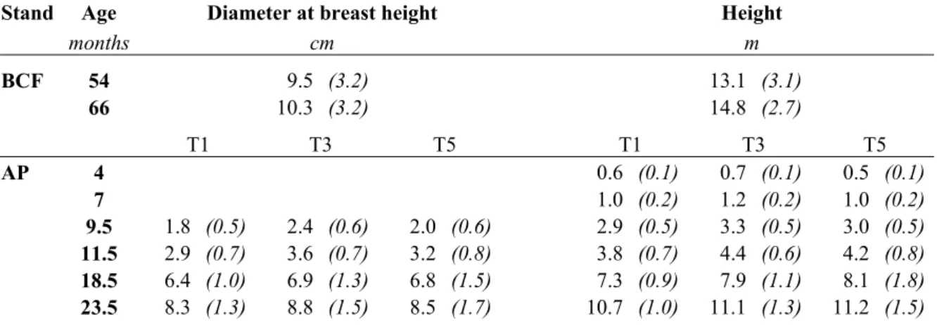
Table 3 Growth in diameter at breast height and height of the Eucalyptus trees

before clear felling (BCF) and after planting (AP). Standard errors are given in parenthesis. ...53

Table 4 E. grandis stand (AP): dry mass and nutrient content in litterfall during the

first and second years of growth in treatments 1, 3 and 5. ...57

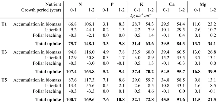
Table 5 E. grandis stand (AP): estimation of the amount of nutrients taken up from

the soil in T1, T3 and T5. ...58

Table 6 E. grandis stand (AP): nutrients taken up and mineralized from the forest

floor or from the harvest residues during the first year of growth. ...59

Table 7 E. grandis (AP): retranslocations of nutrients during leaf senescence (kg

ha-1). The percentage of total annual requirements of the stand is indicated in parenthesis. ...59

Table 8 Point of zero charge (PZC) for some major soil constituents (taken from

Zelany et al. (1996)) ...70

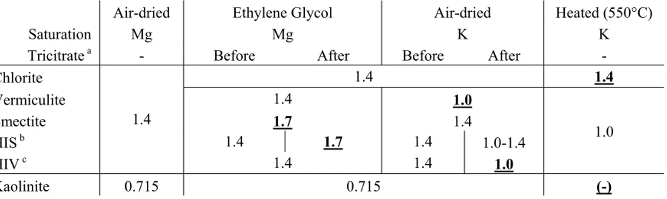
Table 9 Influence of the analytical treatment of a mineralogical clay (saturation

with Mg or K, heating, swelling by Ethylene Glycol, destruction of interlayered Al by tricitrate treatment) on the location of its main peak (nm) on the X-ray chart. The shift of the main peak enables the differentiation and the identification of mineralogical clays. Bold and underlined numbers correspond to key steps in the identification. From Mareschal (2008)...76

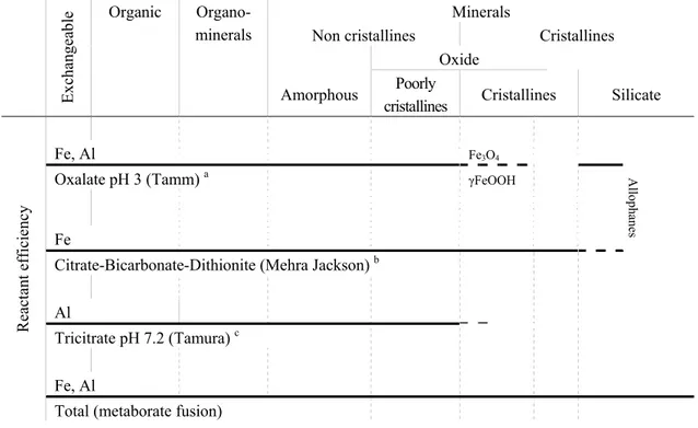
Table 10 Reactant efficiency for aluminium and iron dissolution on different forms

of Al and Fe (organic, organo-minerals or minerals). Adapted from Jeanroy (1983) and Soon (1993). ...77

Table 11 C, N and bulk density models and fitted parameters for data sets SOILBCF-1

& 2 compared to Maquère et al. (2008). ...89

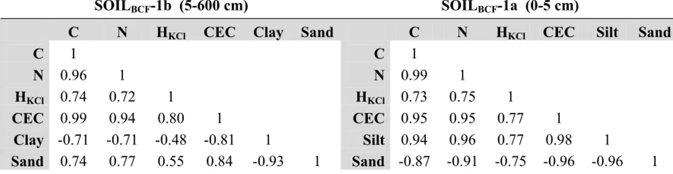
Table 12 Pearson coefficients of correlations calculated for the variables of data sets

SOILBCF-1a and SOILBCF-1b (P<0.05). The matrix for each data set was symmetric so

that only half matrixes are represented...90

Table 13 Linear regressions calculated for the correlated variables of data set

SOILBCF-1a and SOILBCF-1b. The R-square, the F value and its corresponding

probability (Pr>F) are indicated, together with the number of observations (n) and the intercept and slope calculated for the regression. Unless mentioned, intercept and slopes were significantly different from 0 (P < 0.05)...90

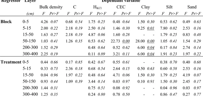
Table 14 One-way ANOVAS performed on the variables of data set SOILBCF-1. The

effect of block and treatment are tested independently on each soil layer (n=9). ...92

Table 15 Mass proportion of total elements, amorphous (Ox) b and free (DCB) c Al

and Fe contents in bulk soil for data sets SOILAP11 and SOIL15m. Standard errors for

Table 16 Pearson correlation coefficients between (i) total Al2O3, Fe2O3 and TiO2

and clay contents, and (ii) total SiO2 and sand contents calculated for data set

SOILAP11, all soil layers taken altogether. Intercept and slope of the corresponding

linear regressions are given for Fe2O3 and SiO2. All slopes and intercepts were

significantly different from zero at P < 0.05. ...98

Table 17 Weight losses (%) measured by thermogravimetry compared to weight

losses from the normative calculation of the clay fraction for pit 3 of data set SOILAP11.106

Table 18 Cation exchange capacity of the clay fraction measured by Sr saturation in

cmol/kg. Standard errors are given in brackets for n≥3. ...108

Table 19 pH in water and in KCl 1 mol L-1, effective cation exchange capacity (CEC

in cmolc kg-1) and saturation in alkaline earth cations (Sat in cmolc kg-1) measured every meter down to a depth of 15 m for data set SOIL15m (n=1)...109

Table 20 Cation exchange capacity (CEC), basic cation exchange capacity (CECb),

and anion exchange capacity at soil pH measured in CaCl2 0.002 mol L-1 (no HCl or

CaOH2 addition) for pit 3 of data set SOILAP11. The pH for which AEC equals CEC

(pH0) together with the pH in KCl 1 mol L-1 and in water are also given...111

Table 21 Langmuir and Freundlich parameters fitted on the experimental data for the

0-5 cm layer (P) and the 200-300 cm layer (S and P). The sum of square errors (SSE) and the number of observations (n) are given. ...113

Table 22 Estimation of the capacity of the soil (in kg ha-1) to retain cation or anion

by non specific adsorption (CEC and AEC) or specific adsorption. For each element, the capacity is calculated for each soil layer from the bulk density of Table 11 and the CEC or AEC of Table 20 fully saturated with the studied element. The charge attributed to each element is +1 for Na, K and N-NH4, +2 for Ca and Mg, +3 for Al, -1

for N-NO3, Cl and P-H2PO4, and -2 for S-SO4. Specific adsorptions are calculated

from Table 21. n.d.=not determined...115

Table 23 MIN3P water balance module: inputs used in the simulations. ...130 Table 24 MIN3P water balance module: outputs used in the simulations. ...130 Table 25 Monitored fluxes: number of collectors and time steps of data acquisition...138 Table 26 Values tested for the input parameters regulating transpiration and

evaporation fluxes in the model. Each parameter is presented in § C.1.1...148

Table 27 Parameter values used for the sensitivity tests. The parameters are

explained in (§ C.1.1.4). ...152

Table 28 Parameters of the root length density model over the studied period. ...155 Table 29 Volumetric water content measured by the TDR probes in treatment 3 and

by soil sampling next to the TDR location...163

Table 30 Soil hydraulic parameters fitted from the water contents and the pressure

heads experimentally recorded during the water drainage experiment. The parameters are explained in § C.1.1.3...165

Table 31 Efficiency of the simulations through EFF1 and EFF2 coefficients (eq (53)

& (54)) for the CFP period. The best simulations are in bold. The simulation kept for the rest of the study is underlined. The maximum sum of square errors recorded for all simulations (SSEmax) and the duration of the simulations (ttot in days) are indicated.

fEV defines the maximum evaporation EVmax (EVmax= fEV ETmax) and zEV the depth

down to which evaporation occurs. ...170

Table 32 Efficiency of the simulations measured by EFF1 and EFF2 (eq (53) &

(54)) for different levels of maximum transpiration Tmax (Tmax= fT ETmax) over the

BCF2 period. SSEmax (min) is the maximum (minimum) sum of square errors (all layers k) of the set of simulations. ttot is the duration of the simulation (days). The grey

cells correspond to simulations for which a peak of water content experimentally measured was not simulated by the model for one of the observation nodes. The best simulations are in bold. The simulation kept for the rest of the study is underlined...172

Table 33 Efficiency of the simulations calculated as EFF1 and EFF2 (eq (53) &

(54)) as a function of the transpiration parameters for the BCF1 period (Tmax=0.6

ETmax). SSEmax (min) is the maximum (minimum) sum of square errors (all layers k)

of the set of simulations. ttot is the duration of the simulation (days). The grey cells

correspond to simulations for which a peak of water content experimentally measured was not simulated by the model for one of the observation nodes. The best simulations are in bold. The simulation kept for the rest of the study is underlined. The simulations of Figure 43 are preceded by *. ...174

Table 34 Number of days (ttot) measured and simulated, sum of squares (SS), sum of

square errors (SSE), root mean square error (RMSE) and mean error (ME) for each simulated period and observation node. ...180

Table 35 Changes in the simulation efficiency (EFF1 and EFF2 coefficients eq (53)

& (54)) with changes in the input parameters ( Table 27) during the CFP period (EVmax=0, Tmax=0). The reference simulation is taken as the average parameter values

of Table 27. SSEmax (min) is the maximum (minimum) sum of square errors (all layers k) of the set of simulations. ttot is the duration of the simulation (days)...184

Table 36 Water balance (mm) for each monitoring depth over each simulated period.

The proportion of the studied flux relatively to the cumulated rainfall during the studied period is given in italic...188

Table 37 Solutions collected and analyzed by ion chromatogry (IC), inductively

coupled plasma (ICP) and dissolved organic carbon analyzer (DOC) over the experimental period in each treatment (T), block (B) and collector (C). The table indicates the combinations of T x B x C collected and analyzed. Superscript f stands for composites collected altogether in the field, whereas superscript l stands for composites prepared in laboratory. Unless mentioned in brackets, all analyses were performed (ICP/IC/DOC). 1:i stands for 1,2,…,i. ZTL=zero-tension lysimeter, TL=tension lysimeter...204

Table 38 Concentration baselines (μmol L-1 and mg L-1 for DOC) calculated for each

element and collector type as the 1st quartile of all blocks and treatments data for the studied period and background ecosystem signal calculated for aboveground collector as the medians of all blocks and treatments data...220

Table 39 Baseline cumulative flux (mmol L-1 and mg L-1 for DOC) for each element,

collector type and collection depth (all blocks and treatments taken altogether for the studied period), and cumulative flux minus baseline cumulative flux for each element, collector type, collection depth and treatment (all blocks taken altogether for the studied period). The maximum cumulative flux is given in bold...222

Table 40 Time (t=Nmonth) and intensity (mmol L-1) of exceptional events in

aboveground solutions collectors (Pi=Rainfall, Th=Throughfall, St=Stemflow). ...224

Table 41 Slope (mmol L-1 or g L-1 for DOC) of the tangent to the cumulative flux

curve at the end of the experimental period for each collector type (ZTL=zero tension lysimeter, TL=tension lysimeter), collection depth and treatment (T). The slopes are given in bold when there value was above the threshold for nutrient flux SC’t=1 mmol

month-1 (0.06 g month-1 for DOC). ...261

Table 42 Fluxes entering or leaving the studied system (system A of Figure 2). ...272 Table 43 Stocks of the studied system at clear felling (T0) and two years after

planting (Tf)...275

Table 44 Pearson coefficients of correlation calculated for fresh soil water extracts at

age two years (AP24) in treatments 1 (T1), 3 (T3) and 5 (T5) compared to the reference treatment R (part of the previous stand (BCF) kept uncut). Only the coefficients corresponding to P<0.05 are given. ...285

Table 45 Input and output budgets calculated from the clear felling (CF) until age

two year (AP24) for N, P, K, Mg and Ca, and partially for Al and S in treatments 1, 3

and 5. Total inflow entering the system (by fertilization and bulk deposits) and total outflow leaving the system by drainage at a depth of 3 m are given, together with changes in stocks measured after clear felling and at age two years. The stem is the biomass fraction which may be exported at clear felling. Abbreviations are detailed in Table 43. ...292

ANNEX

Table A-1 Total analysis of the sewage sludge applied in the experiment (ND = Not

Detected). ...309

Table A-2 Total analyses of the mineral fertilizers (na= not analyzed) ...310 Table A-3 Time course of the nutrient accumulation in aboveground biomass at the

end of the rotation of the E. saligna stand...311

Table A-4 Biomass and nutrients accumulation in E. grandis trees in T1, T3 and T5

from age 6 months to age 2 years...312

Table A-5 Chemical and physical characteristics of data set SOILBCF...315

Table A-6 Chemical and physical characteristics of data set SOILAP11: C & N

contents, pH and CEC, and particle-size distribution...316

Table A-7 Chemical and physical characteristics of data set SOILAP11: Al an Fe

extractions and total analysis...317

Table A-8 Al an Fe extractions and total analysis of soil fractions of data set SOILAP11318

Table A-9 Effects tested on model A-5 and results of the F-tests. p1 and p2 are the

number of parameters of the models, n the number of observations. Fobs calculation is

given in eq. A-6 and Ftab is the theoretical value given in the Fischer’s table. ...324

Table A-10 Repartition of the stand and stem flow sampling devices into basal

Table A-11 Growth parameters (eq. A-7) used to estimate the girth breast height (CBH) of the trees equipped with stemflow monitoring devices after clear felling...325

Table A-12 Intercepts, slopes and R-square of the linear regressions relating the

water contents measured for a given TDR probe to the average water content for all probes of the experiment. ...331

Table A-13 Average cumulative fluxes and standard deviations (when n≥3)

calculated from the clear felling (Nmonth=9) to the end of the experimental period

(Nmonth=37) for cations and anions measured in soil solutions for each collector type,

collection depth and treatment...335

Table A-14 Specific extractions performed on soils at age 2 years after planting:

reference stand kept uncut. Mean and standard errors (when n≥3) are given. ...337

Table A-15 Specific extractions performed on soils at age 2 years after planting:

Treatment 1. Mean and standard errors (when n≥3) are given...338

Table A-16 Specific extractions performed on soils at age 2 years after planting:

Treatment 3. Mean and standard errors (when n≥3) are given...339

Table A-17 Specific extractions performed on soils at age 2 years after planting:

“Je suis allé faire parler le cuir usé d’une valise entreposée sous la poussière terre d’une vieille remise

G

Each year the area of fast-growing tree plantations in the world expands by around one million hectares as a result of the population growth and the steady increase in the per capit consumption of wood and wood-based products (paper, wood-fibre panels, …) (FAO, 2006). Fast-wood plantations are intensively managed commercial plantations, set in blocks of a single species, which produce industrial round wood at high growth rates (mean annual increment of no less than 15 m3 per hectare) and which are harvested in less than 20 years. These can be large-scale estates owned by companies or a concentration of a large number of small- to medium-scale commercial woodlots owned by smallholders (Cossalter and Pye-Smith, 2003). Eucalyptus is the most widely planted tree genus in the tropics, E. grandis, E. saligna and E urophylla are the main planted species in tropical and subtropical climate (FAO, 2006).

Some 30 years ago, Brazil became the first country in South America to establish large fast-wood plantations. Plantations represent 5.74 millions ha out of the 477.7 millions ha of Brazilian forests, of which 28.3 % are concentrated in the states of Minas Gerais and São Paulo. Eucalyptus count 3.55 millions ha and Pinus 1.82 millions ha. Planted forests account for 4.33 millions employs (SBS, 2007). Eucalyptus plantations mainly supply the pulp and metallurgical industries with wood and charcoal. The rotation length is classically 7 years, 2 or 3 successive rotations are generally performed before the stand is reformed. The yields are among the best in the world and reach classically 40 to 50 m3 ha-1 year-1 (Goncalves et al., 2004).

The planting of large areas of eucalypts, acacias, pines and poplars has sparked off bitter controversy, especially in the developing world. For plantations propronents, these have countless virtues: they regulate water cycle, convert sunlight and carbon dioxide into wood and oxygen, stabilise steep slopes against erosion, constitute habitat for animals and micro-organisms, and provide employment to local communities together with timber, firewood, resins and other products. On the other hand, the opponents to fast-wood plantations argue that they are replacing natural forests, that they are threat to biodiversity, to water resources and to soil fertility, that genetically modified tree crops will lead to problems in the future, and that they cause land tenure and conflict with local communities (Cossalter and Pye-Smith, 2003). Fast-wood plantation companies are under increasing pressure from non governmental organizations so that nowadays in Brasil, most of them

are willing to assess the ecological and social impacts of their activity. About 2.25 millions ha of Brazilian plantations are certified FSC (Forest Stewardship Council) and outgrower or joint-venture schemes are being developed in most Brazilian states (SBS, 2007).

In terms of soil sustainability, one major concern regards soil fertility since most of these plantations are managed in short rotations and large amounts of nutrients contained in boles are removed from soils on each harvest (Cossalter and Pye-Smith, 2003; Nambiar et al., 2004). In terms of nutrient cycling, fast-wood plantations behave like most agricultural crops, in that they remove minerals from the soil. As they are frequently established on low fertility soils, fast-wood crops nearly always require applications of fertilizer if they are to sustain high biomass productions. Most of these are mineral fertilizers but increasing production of sewage sludge from wastewater treatment plants of urbanized areas has encouraged the use of sewage sludge as fertilizers. The stakes are for industrials to optimize these fertilizations to supply the stand requirements at minimal cost and for environmentalists to guaranty that they are adapted to maintain soil fertility without polluting underground waters.

Eucalyptus response to P, K and B fertilizations has been widely studied in Brazil

(IPEF, 2004) but less attention was put on N fertilizers although they are applicated in industrial plantations (from 100 to 200 kg ha-1 for each rotation). It was already observed in the Congo that long-term silviculture of Eucalyptus led to imbalanced N budgets (Laclau et al., 2005a), which may result in soil organic nitrogen impoverishment. A strong response to N fertilizers was also observed in Australia and since a few years in Brazil (Corbeels et al., 2005; Goncalves et al., 2004). More precise knowledge of the nitrogen cycle in Eucalyptus plantations is required to (i) maintain high yields of production at reduced cost without impoverishing the soils, and (ii) to prevent water pollution with nitrates.

Water consumption of large fast-wood plantations has been widely discussed. These plantations reduce annual water yields, especially when they replace grasslands and farmland, thus leaving less water available to other users, and often reduce stream flow during the dry season. However, where there is abundant rainfall, their effect on water yields may be insignificant (Cossalter and Pye-Smith, 2003). The influence of Eucalyptus plantations on the water resource has been intensively studied at the catchment scale in particular in Brazil (Camara and Lima, 1999; Lima, 1996; Lima et al., 1996) and in South Africa (Bosch and Smith, 1989; LeMaitre and Versfeld, 1997; Prinsloo and Scott, 1999;

Scott and Smith, 1997). The Eucalyptus consumption in water was also studied at the tree scale by ecophysiological monitoring (Benyon, 1999; Bevilacqua et al., 1997; David et al., 1997b; Dye, 1996; Kallarackal and Somen, 1997; Stape et al., 2004), but less information is available regarding the water dynamics in soils and the chemistry of soil solutions.

The problems related to plantations are often site-specific, and the way in which they are planned and managed is of paramount importance. The impact of plantations is generally a function of the characteristics of (i) the land-use they replace, (ii) the soil and climate of the site, (iii) the size of the planted area, (iv) the silvicultural practices (soil preparation, stocking density, fertilization, length of rotation,…), and (v) the species composition (Cossalter and Pye-Smith, 2003). Site-specific studies are thus needed to identify local determinisms of plantation dynamics which may serve as basis for further generalisation. From a scientific point of view, fast-wood monospecific plantations form simplified and highly homogeneous systems observable at a short time scale (7 years for a whole rotation in Brazil for example). They are thus particularly well adapted for model building, parameterization and validation.

Desorption Desorption Soil Substratum Forest Floor Tree uptake Tree uptake Dry and wet deposition

Litterfall Restitution (harvest residues) Export (harvest) Foliar leaching and absorption Throughfall Stemflow Drainage and capillary rise Mineral weathering Mineral weathering Precipitation Fertilization Adsorption Adsorption Mineralization Mineralization Immobilization (OM+microbial biomass) Immobilization (OM+microbial biomass) Root exudation Surface run-off Desorption Desorption Soil Substratum Forest Floor Tree uptake Tree uptake Dry and wet deposition

Litterfall Restitution (harvest residues) Export (harvest) Foliar leaching and absorption Throughfall Stemflow Drainage and capillary rise Mineral weathering Mineral weathering Precipitation Fertilization Adsorption Adsorption Mineralization Mineralization Immobilization (OM+microbial biomass) Immobilization (OM+microbial biomass) Root exudation Surface run-off

Figure 1 Processes of nutrient transfers occurring within forest ecosystems.

A comprehensive approach is currently being conducted at the University of São Paulo to study the biogeochemical cycles of nutrients in Eucalyptus grandis plantations. This

project is developed at the ecosystem level in an experimental stand representative of large areas of plantations in Brazil. The overall aim of the study is to assess the consequences of silviculture, and more particular of different N fertilizer inputs, on water quality and long-term soil fertility by measuring water and nutrient fluxes throughout the ecosystem ( Figure 1) and establishing the input-output budgets of nutrients in the soil for the whole rotation (Ranger et al., 2002).

As part of this study, the present thesis focused on the interactions between the soil matrix and the soil solutions during the first two years of growth of the Eucalyptus stand.

The main objective was to study the dynamics of the soil and forest floor solutions (system D of Figure 2) and to set hypotheses on the main fluxes driving its chemical composition (fluxes of system D on Figure 2). The underlying hypotheses were that in these deep weathered tropical soils, the reactions of adsorption/desorption on the soil surface are key controls of the dynamics of soil solution, but that the weathering of the mineral phase contributes little to nutrient release in soil solution. The thesis thus aimed at:

• identifying the determinisms driving the chemistry of the soil solution,

• quantifying the water and nutrient fluxes leaving the ecosystem by deep drainage and thus rule on the risks of groundwater pollution,

• preparing reactive transport modeling and assess its feasibility, using the model already in use at the INRA-BEF laboratory, MIN3P (Gerard et al., 2004; Mayer et al., 2002).

The study was organized in different parts which settled the structure of the present dissertation:

• the fertilization experiment is presented in part A, together with the dynamics of the vegetation over the studied period, which was not part of this thesis but helps to understand the dynamics of the soil solution,

• the potential interactions between the soil solid phase and the soil solution were then studied (potential fluxes of mineral weathering and adsorption/desorption indicated in Figure 2) (part B),

• the chemistry of the soil solution was studied and the nutrient fluxes leaving the soil system by deep drainage were calculated (part D),

• finally, the mass budgets of nutrients within the ecosystem (system A of Figure 2) were assessed to check the validity of the hypotheses formulated in parts B, C and D on the drivers of the soil solution chemistry (part E).

The thesis focuses on the mineral forms of the elements brought by the fertilizers (in particular for N, P, K, Ca, Mg); the organic part of the systems was not presently studied but was discussed in part E.

Since most fluxes of system D (especially those occurring in soils) are difficult to measure experimentally, the hypotheses formulated in parts A, B, C and D were not directly checked by measuring the corresponding fluxes. In part E, we checked by simple mass budget wether these hypotheses were consistant with the main transfers occurring during the experimental period among storage compartments. Mass budgets were performed on system A of Figure 2, for which the main fluxes entering or leaving the system were experimentally available. Part E does not establish nutrient fertility budgets of the experiment.

Throughout the thesis, soil surface represents the contact area between soil constituents and soil solution. For practical purposes, the name “fertilizer” represents mineral fertilizer and sewage sludge applications

Each part of the thesis is self-consistant. A detailed introduction presents, for each one of them, the main questions at stakes. Specific material and methods, results and discussions, and conclusions are developed within each part.

Figure 2 Schematic mass budgets for different sub-systems as part of the ecosystem:

system “tree+ forest floor+soil+soil solution” (A), system “tree” (B), system “forest floor+soil+soil solutions” (C), system “forest floor solutions and soil solutions” (D). Fluxes entering or leaving each system are represented in red arrows. The thesis focuses on the dynamics of system D. Mass budgets were performed for system A. Systems A and C are equivalent once the root uptake is calculated as the sum of litterfall plus nutrient accumulation in trees.

PART A

P

REAMBLE

T

HE EXPERIMENT

:

S

ITE CHARACTERISTICS

E

XPERIMENTAL DESIGN

Figure 3 Localization of the experimental station of Itatinga (São Paulo state, Brazil)