Heterogeneous Structural Organization of Polystyrene Fibers Prepared by Electrospinning

(1)

Université de Montréal

Heterogeneous Structural Organization of Polystyrene Fibers Prepared by

Electrospinning

présenté par

Anna Gittsegrad

Département de chimie Faculté des arts et des sciences

Mémoire présenté à la Faculté des études supérieures et postdoctorales en vue de l’obtention du grade de maître ès sciences (M.Sc.) en chimie

Janvier 2018 © Anna Gittsegrad, 2018

(2)

i

RÉSUMÉ

L'électrofilage est une technique utilisée pour la préparation de fibres avec des diamètres allant de quelques micromètres jusqu'à des centaines de nanomètres à partir d'une solution polymère enchevêtrée dans un solvant volatil. Les fibres électrofilées sont formées sous l'influence de grandes forces d'étirement, qui contribuent à une évaporation extrêmement rapide du solvant, une orientation moléculaire élevée et une structure moléculaire hors d’équilibre. Il a été démontré que ces matériaux présentent des propriétés distinctes par rapport aux matériaux massiques. Dans ce travail, le comportement thermique des fibres polystyrène (PS) électrofilées à partir de différents solvants a été étudié à l'aide de calorimétrie différentielle à balayage (DSC) modulée en température. Une analyse détaillée du système PS/CHCl3 ainsi que l'utilisation de trois masses moléculaires et de différentes concentrations a révélé la présence de deux phases dans les fibres de PS avec une phase secondaire moins dense que la phase normale. Ces résultats ont été corrélés au modèle précédemment proposé de l'organisation de la chaîne « cœur-couronne » avec la couronne mince partiellement désenchevêtrée et un cœur enchevêtré en masse. Des mesures supplémentaires de spectroscopie par une technique qui combine la spectroscopie infrarouge avec le microscope à force atomique (AFM-IR) à l’échelle de fibre unique ont démontré que les bandes IR associées à un désenchevêtrement partiel dans des chaînes sont situées essentiellement au bord de la fibre. Différents solvants, le tétrahydrofurane (THF), la méthyléthylcétone (MEK) et le diméthylformamide (DMF) ayant des points d'ébullition différents ont été utilisés pour électrofiler les fibres de PS et ont généré un comportement à deux phases pour toutes les masses moléculaires et concentrations. La morphologie des fibres PS électrofilées provenant de différents solvants a également été étudiée. De plus, le recuit thermique des fibres de PS dans de multiples conditions a été effectué qui a permis de mieux comprendre le comportement thermique inhabituel et une organisation en deux phases des fibres PS. Enfin, ces résultats ont été corrélés avec le modèle « cœur-couronne » pour l'organisation des chaînes au sein des fibres et les hypothèses de ce modèle ont été révisées.

(3)

ii

Mots-clés: Électrofilage, fibres polymères, polystyrène, morphologie, comportement

(4)

iii

ABSTRACT

Electrospinning is a common technique used for preparing fibers with diameters ranging from a few micrometers down to hundreds of nanometers from an entangled polymeric solution in a volatile solvent. Electrospun fibers are formed under the influence of large stretching forces, therefore contributing to extremely fast solvent evaporation, high molecular orientation and out-of-equilibrium structure. These materials have been shown to exhibit distinct properties when compared to bulk materials. In this work, the thermal behavior of polystyrene (PS) fibers electrospun from different solvents as well as using three molecular weights and different concentrations was studied using temperature modulated differential scanning calorimetry (DSC). A detailed analysis of the PS/CHCl3 system revealed the presence of two phases within PS fibers with a secondary phase being less dense than the normal phase. The observations were correlated to the previously proposed model of core-shell chain organization with a partially disentangled thin shell and a bulk entangled core. Additional spectroscopic measurements by atomic force microscopy infrared spectroscopy (AFM-IR) at the single fiber scale demonstrated that IR bands associated with partial disentanglement in chains are located mainly at the edge of the fiber. Different solvents, tetrahydrofuran (THF), methyl ethyl ketone (MEK) and dimethylformamide (DMF) having different boiling points were used to electrospin PS fibers that featured two-phase behavior at all molecular weights and concentrations. The morphology of PS fibers electrospun from different solvents was also studied. Moreover, the thermal annealing of PS fibers under multiple conditions was performed that shed light on the unusual thermal behavior and a better understanding of the two-phase organization of the PS fibers. Finally, these results were correlated with the core-shell model for the chain organization within fibers and the hypotheses of this model were revised.

Keywords: Electrospinning, polymer fibers, polystyrene, morphology, thermal

(5)

iv

LIST OF FIGURES

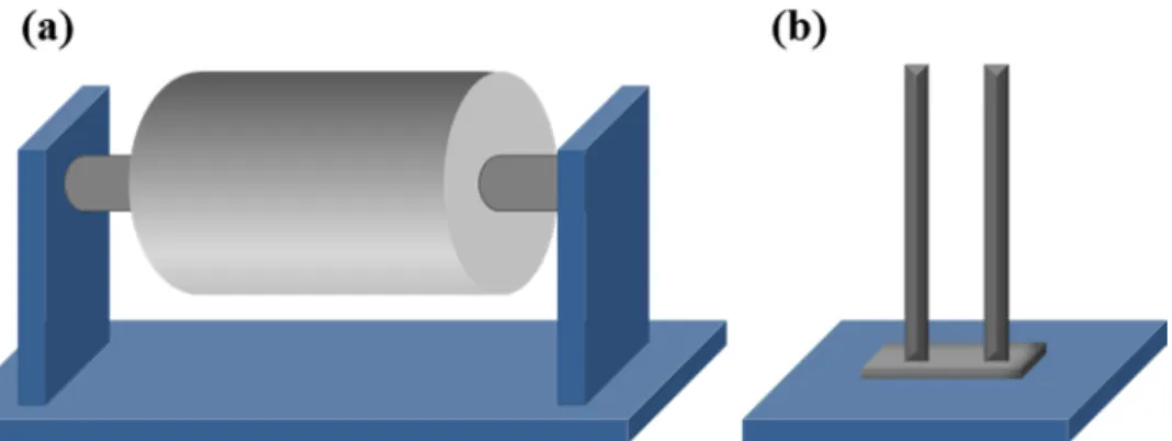
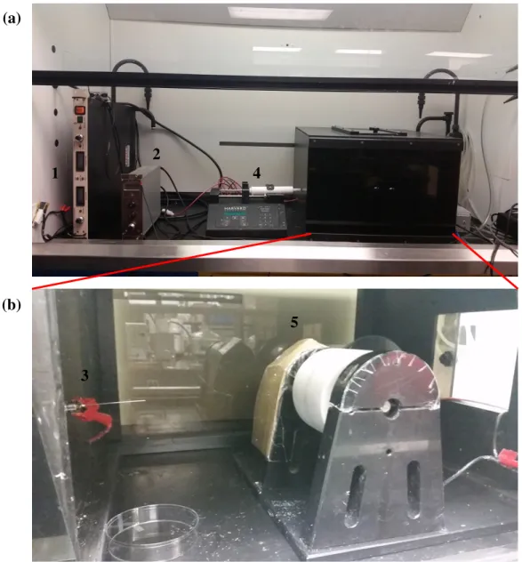
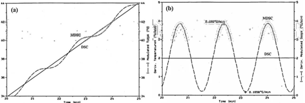
Figure 1.1 Typical setup for an electrospinning experiment. ... 5 Figure 1.2 Schematic representation of the Taylor cone. ... 6 Figure 1.3 (a) Diagram representing the onset and development of bending instabilities and (b) image of the bending instability near the end of the straight part of the jet.. ... 8 Figure 1.4 Effect of the applied voltage on the formation of the Taylor cone.. ... 10 Figure 1.5 Schematic representation of rotating drum collector (a) and a parallel rods collector for electrospinning. ... 12 Figure 1.6 Physical representations of three solution regimes (a) dilute, (b) semidilute unentangled and (c) semidilute entangled. ... 15 Figure 1.7 Schematic representations of (a) radial solvent evaporation of the solvent from the jet, and possible fiber morphologies: (b) surface pores, (c) internal pores, (d) elongated pores or wrinkled fibers and (e) dumbbell shaped fibers. ... 21 Figure 1.8 Generalized dependence of Young’s modulus, strength and toughness on fiber diameter... 22 Figure 1.9 Direct correlation between the diameter dependence of relative modulus and molecular orientation. ... 23 Figure 1.10 Schematic representation of the core-shell morphology and the polymer density gradient due to the solvent evaporation during the electrospinning process. ... 28 Figure 1.11 Schematic representation of partially disentangled shell and bulk entangled core within electrospun fibers.. ... 29 Figure 2.1 Photographs of the electrospinning setup used in our laboratory. (a) general view including high voltage power sources (1 and 2) and automated injector (4) and (b) close look at the needle (3) and rotating disk collector (5). ... 34 Figure 2.2 Temperature as a function of time (a) and heating rate as a function of time (b) for typical DSC and TMDSC experiment. ... 35 Figure 2.3 Modulated heating rate (input) and modulated heat flow (output) for the TMDSC experiment. ... 36 Figure 2.4 Deconvoluted heat flow signals (total, reversing and nonreversing) obtained by TMDSC. Example is presented for quenched poly(ethylene terephthalate) (PET) sample. The total heat flow signal (green), equivalent to the conventional DSC signal, shows the glass transition, the cold crystallization exotherm, and the melting of the

(8)

vii

formed crystals. In the reversing (blue) and nonreversing (red) components, in this region endothermic melting (in the reversing heat flow) and exothermic (re)crystallization (in the nonreversing heat flow) compete, resulting in a net ‘zero’ effect in the total heat flow. The glass transition is observed in the total and reversing heat flow signal, whereas the nonreversing heat flow signal reveals the presence of enthalpic recovery peak otherwise not seen in the total heat flow.. ... 38 Figure 3.1 (a) SEM image of PS fibers electrospun from a 12.5% w/v chloroform solution (Mw = 900 000 g/mol) (the scale bar is 10 µm) with the corresponding DSC thermogram for the first heating run (b) and the zoomed region around Tg (c). ... 42 Figure 3.2 TMDSC thermograms of PS fibers electrospun from a 12.5% from chloroform solution (Mw = 900 000 g/mol) showing the total, reversing and nonreversing heat flow for the first heating run (solid line) and the second heating run (dotted line). ... 44 Figure 3.3 (a) Estimate of ∆Cp using two possible baselines for the total heat flow signal (first and second heating runs) and for the reversing heat flow. (b) Corresponding measurements of Tg. ... 45 Figure 3.4 Representation of sub-Tg annealing temperatures for PS fibers electrospun from 12.5% w/v chloroform solution (Mw = 900 000 g/mol). ... 47 Figure 3.5 TMDSC thermograms of PS electrospun from 12.5% from chloroform solution (Mw = 900 000 g/mol) showing the total, reversing and nonreversing heat flows following different sub-Tg annealing temperatures and times. ... 48 Figure 3.6 The position of the normal (peak 1) and secondary (peak 2) enthalpic relaxation peaks as a function of annealing conditions. ... 49 Table 3.1 Concentrations used to electrospin PS fibers of different molecular weights from chloroform solutions. ... 50 Figure 3.7 TMDSC thermograms of PS electrospun from 12.5 and 10% from chloroform solution (Mw = 900 000 g/mol) and 10 and 8% (Mw = 2 000 000 g/mol) showing the total, reversing and nonreversing heat flows. Solid lines represent the first heating run and dotted lines the second heating run. ... 51 Figure 3.8 TMDSC thermograms of PS electrospun from 12.5 and 10% from chloroform solution (Mw = 900 000 g/mol) and 10 and 8% (Mw = 2 000 000 g/mol) annealed at 75 ˚C for 3h showing the total, reversing and nonreversing heat flows. Dashed lines represent the first heating run and dotted lines the second heating run without annealing. ... 52

(9)

viii

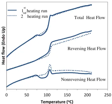
Figure 3.9 TMDSC thermograms of PS electrospun from 12.5% (Mw = 900 000 g/mol) and 25 and 22.5% (Mw = 210 000 g/mol) chloroform solution showing the total, reversing and nonreversing heat flows. Solid lines represent the first heating run and dotted lines the second heating run. ... 53 Figure 3.10 Effect of the molecular weight on the glass transition temperature of PS electrospun fibers (measured by TMDSC). ... 54 Figure 3.11 TMDSC thermograms of PS fibers electrospun from 12.5% from chloroform solution (Mw = 900 000 g/mol) and 25 and 22.5% (Mw = 210 000 g/mol) annealed at Tg – 30 ˚C for 3 h showing the total, reversing and nonreversing heat flows. Dashed lines represent the first heating run and dotted lines the second heating run. ... 56 Figure 3.12 Schematic representation of the effect of annealing on the enthalpy-temperature curve showing the normal phase (red) and the secondary phase (blue) without annealing (a) and for the annealing conditions at 45 °C for 48h (b), at 65 °C for 3h and 24h, at 75 °C for 3h (d), at 75 °C for 24h (e) and at 85 °C for 3h (f). ... 59 Figure 3.13 (a) TMDSC curves of PS fibers electrospun from chloroform solution showing the nonreversing heat flow signal for three molecular weights. ( ) is the first heating run for fibers annealed at 75 °C for 3h and the ( ) are the results of identical annealing conditions on samples whose thermal history was previously erased by heating well above Tg. (b) Enthalpic relaxation of the samples with erased thermal history annealed at 75 °C for 3h. ... 61 Figure 3.14 Enthalpic relaxation of the fibers annealed at 75 °C for 3h as a function of molecular weight and concentration for (a) the normal phase (∆H1) and (b) the secondary phase (∆H2). ... 62 Figure 3.15 Schematic representation of the volume fraction of the secondary and the normal phases in PS fibers as a function of molecular weight ... 63 Figure 3.16 (a) AFM image of a single PS fiber electrospun from a 10% w/v chloroform solution and transferred onto a BaF2 substrate. (b) IR spectra of the single PS fiber shown in the AFM image. The color markers on the AFM image indicate the approximate position of the AFM tip for each IR spectrum. The two red spectra are taken at the edge of the fiber. ... 66 Figure 3.17 (a) AFM topographic image of a single PS fiber electrospun from a 10% w/v chloroform solution transferred onto a BaF2 substrate; corresponding chemical maps of the 1449 cm-1 band (b) and the 1262 cm-1 band (c). ... 68 Figure 3.18 Chemical mapping of the 1449 cm-1 (top) and 1262 cm-1 band (bottom) of PS single fibers electrospun from 10% w/v chloroform solutions transferred onto a BaF2

(10)

ix

substrate for different annealing conditions (a) 75 °C for 3 h, (b) 75 °C for 24 h and (c) 150 °C for 3 h, and (d) corresponding IR spectra. ... 70 Figure 3.19 Schematic representation of the two phase system in the cross-section of PS fibers with partially disentangled chains in the outer shell and bulk entanglement in the core. The effect of different annealing conditions on the internal microstructure is presented where darker color represents a denser phase and lighter color a less dense phase. ... 71 Figure 3.20 SEM micrographs of PS fibers showing different morphologies obtained by changing the solvent and solution concentration. The scale bars are 10 and 1 µm for the global and the zoomed images, respectively. ... 73 Figure 3.21 Two mechanisms of the formation of grooved fibers: void-based formation (a) and wrinkles formation (b). ... 74 Figure 3.22 Schematic representation of the structural characteristics of the jet (1) immediately after ejection from the needle, (2) during the whipping and stretching and (3) upon drying on the collector showing the effect of low (A) and high (B) relative humidity. ... 76 Figure 3.23 Schematic representation of the progression of the collapse of the skin of the jet to form a ribbon-shaped fiber. ... 77 Figure 3.24 Diameter of the fibers as a function of concentration and molecular weight for fibers electrospun in four different solvents: chloroform (a), THF (b), MEK (c), and DMF (d). The error bars represent the average of 30 measurements. ... 79 Figure 3.25 TMDSC thermograms of PS (Mw = 900 000 g/mol) electrospun from 12.5 % w/v chloroform (black), 12.5 % w/v THF (red), 10 % w/v MEK (blue) and 15 % w/v DMF (green) solutions showing the total (a), reversing (b) and nonreversing (c) heat flows. Solid lines represent the first heating run and dotted lines the second heating run. ... 81 Figure 4.1 (a) Chemical mapping of the 1449 cm-1 (top) and 1262 cm-1 band (bottom) of PS single fiber electrospun from 20% w/v DMF solution (Mw = 210 000 g/mol) transferred onto a BaF2 substrate and (b) corresponding IR spectra taken at two tip positions at the edge of the fiber. ... 86 Figure 4.2 DSC thermograms of PS (black) and PS/PPO at different weight fractions (blue). Solid line represents the first heating run and the dotted line the second heating run. ... 88

(11)

x

Figure A1 SEM micrographs of PS fibers electrospun from chloroform solutions at three molecular weights, 210 000 g/mol (a), 900 000 g/mol (b) and 2 000 000 g/mol (c) with two concentrations for each molecular weight. ... 90 Figure A2 SEM micrographs of PS fibers electrospun from THF solutions at two molecular weights, 900 000 g/mol (a) and 2 000 000 g/mol (b) with two concentrations for each molecular weight. ... 91 Figure A3 SEM micrographs of PS fibers electrospun from MEK solutions at two molecular weights, 900 000 g/mol (a) and 2 000 000 g/mol (b). ... 91 Figure A4 SEM micrographs of PS fibers electrospun from DMF solutions at three molecular weights, 210 000 g/mol (a), 900 000 g/mol (b) and 2 000 000 g/mol (c) with two concentrations for each molecular weight. ... 92 Figure A5 TMDSC thermograms of PS electrospun from 12.5 and 10% from THF solution (Mw = 900 000 g/mol) and 8 and 6.5% (Mw = 2 000 000 g/mol) showing the total (a), reversing (b) and nonreversing (c) heat flows. Solid lines represent the first heating run and dotted lines the second heating run... 93 Figure A6 TMDSC thermograms of PS electrospun from 10% from MEK solution (Mw = 900 000 g/mol) and 5% (Mw = 2 000 000 g/mol) showing the total (a), reversing (b) and nonreversing (c) heat flows and the annealed fibers at 75 °C for 3h. Solid lines represent the first heating run, dashed lines represent the annealed fibers and dotted lines the second heating run. ... 94 Figure A7 TMDSC thermograms of PS electrospun from 25 and 20% from DMF solution (Mw = 210 000 g/mol), 20 and 15% (Mw = 900 000 g/mol) and 15 and 10% (Mw = 2 000 000 g/mol) showing the total (a), reversing (b) and nonreversing (c) heat flows. Solid lines represent the first heating run and dotted lines the second heating run. ... 95 Figure A8 TMDSC thermograms of PS electrospun from 12.5 and 10% from THF solution (Mw = 900 000 g/mol) and 8 and 6.5% (Mw = 2 000 000 g/mol) annealed at 75°C for 3h showing the total (a), reversing (b) and nonreversing (c) heat flows. Dashed lines represent the first heating run and dotted lines the second heating run. ... 96 Figure A9 TMDSC thermograms of PS electrospun from 25 and 20% from DMF solution (Mw = 210 000 g/mol), 20 and 15% (Mw = 900 000 g/mol) and 15 and 10% (Mw = 2 000 000 g/mol) annealed at Tg – 30 ˚C for 3h showing the total (a), reversing (b) and nonreversing (c) heat flows. Dashed lines represent the first heating run and dotted lines the second heating run. ... 97

(12)

xi

LIST OF TABLES

Table 3.1 Concentrations used to electrospin PS fibers of different molecular weights from chloroform solutions. ... 50 Table 3.2 Properties of the four solvents used in this work. ... 73

(13)

xii

LIST OF ABBREVIATIONS

AFM atomic force microscopy

ATR-IR attenuated total reflection infrared spectroscopy

c concentration

c* limiting concentration

ce critical entanglement concentration

DMF dimethylformamide

DSC differential scanning calorimetry

EID excess of isotropic intensity

Mc critical molecular weight

MEK methyl ethyl ketone

Mw molecular weight

PCL poly(ε-caprolactone)

PDI polydispersity index

PGS poly(glycerol sebacate)

PHBHx poly[(R)-3-hydroxybutyrate-co-(R)-3-hydroxyhexanoate]

PPO poly(propylene oxide)

PS polystyrene

PVA poly(vinyl alcohol)

PVC poly(vinyl chloride)

PVDF poly(vinylidenefluoride)

PVDF-PHFP poly(vinylidene fluoride-hexafluoropropylene) PVME poly(vinyl methyl ether)

SEM scanning electron microscopy

Tc crystallization temperature

Tg glass transition temperature

THF tetrahydrofuran

(14)

xiii

TMDSC temperature modulated differential scanning calorimetry

Vc critical potential

∆Cp specific heat capacity

(15)

xiv

ACKNOWLEDGEMENTS

First and foremost, I would like to thank my thesis advisors, Prof. Christian Pellerin and Prof. C. Geraldine Bazuin. I would like to express my gratitude to them for their patience, motivation, enthusiasm and immense knowledge, and for allowing this thesis to be my own work, but steering me in the right the direction whenever they thought I needed it. I am grateful for all of the opportunities I was given to conduct my research on a variety of projects.

Besides my advisors, I would like to thank Prof. Robert E. Prud’homme for his support, guidance and collaborative work.

A very special thanks goes out to Marie Richard-Lacroix and Elise Siurdyban for their substantial contribution to our collaborative work, ideas and energy that led our joint project to good results.

I would like to specifically thank Sylvain Essiembre for his time, training and help with DSC instruments, providing me with necessary information to succeed in my project and deepen my instrumental knowledge.

I am grateful to all current and previous members of Pellerin, Bazuin and Prud’homme research groups that have contributed immensely to my personal and professional time at Université de Montréal.

(16)

1

Chapter 1 INTRODUCTION

1.1 Electrospinning of polymer fibers

Synthetic and natural polymers are being increasingly employed as structural materials and active functional systems. This technological development has often aimed to miniaturize commonly used systems and components to the micro- and nano-scale and to generate polymeric materials with superior performance that are improvements over the existing ones. At the same time, the development of characterization methods with enhanced spatial resolution allows studying complex systems, such as membranes, ultrathin polymer films and carbon nanotubes with unprecedented detail. Among these materials are polymeric fibers prepared by the electrospinning method. While the process of fiber preparation by electrospinning is relatively simple, the study of the out-of-equilibrium molecular organization within these fibers, which results in unique properties, is an active area of research.

Generally speaking, spinning of polymer fibers involves the extrusion of a polymer melt, solution or gel through a spinneret to generate continuous filaments.1 The oldest process is wet spinning, where a dissolved polymer is pushed through a spinneret submerged in a chemical bath filled with non-solvent. When extruded, fibers precipitate from solution and solidify. A variation of wet spinning is dry jet-wet spinning. In this technique, the polymer solution is extruded into an air gap under heat and pressure before entering the coagulation bath. It is often used to produce high performance fibers possessing a liquid crystalline structure. Another solution-based fiber-forming method is

dry spinning, in which fibers solidify through solvent evaporation with hot air or inert

gas. It is simpler, since the drying and solvent recovery steps are eliminated. In melt

(17)

2

A thin stream of liquid then drops onto a spinning wheel and is cooled, resulting in rapid solidification. This process generates fibers with a variety of cross-sectional shapes.1

Electrospinning is another method that allows preparing ultrathin polymer fibers that has become popular since the mid-1990s. It is based on the uniaxial stretching and fast solvent evaporation of the jet derived from a semi-dilute polymer solution.2 Unlike other spinning processes, it employs electrostatic repulsion between surface charges and attraction to an oppositely charged collector under a large electric field instead of mechanical forces in order to generate filaments, leading to a reduction in diameter of the jet and the resulting fibers. In fact, fibers with much smaller diameter, down to micrometer range or even tens of nanometers, can be readily obtained.3 High-volume production of fibers with relatively long length and with either solid or hollow/porous interiors can be achieved because electrospinning represents a continuous process in which the elongation is attained through the application of an external electric field.

Electrospinning is in fact an old technique and its development has originated in the 18th century. The first studies were performed in 1745 by Bose, who was able to produce aerosol by applying high electric potentials to drops of fluids.4 In 1882, Lord Rayleigh has quantified the amount of charges that are necessary to overcome the surface tension of a drop.5 Later, in 1902, Cooley and Morton were issued the first patent for devices that allowed spraying a liquid by applying electrical fields.6-7 The term electrospinning or “electrostatic spinning” was commonly used only at the end of 20th century. However, its origins lay in a crucial patent published by Formhals in 1934, describing for the first time the setup for the electrospinning of polymeric filaments.8 In the 1960s, Taylor has demonstrated that under an electric field, a conical interface between two fluids can exist in equilibrium, with a semi-vertical angle of around 49.3o.9 He then proposed a theory of electrically driven jets establishing that the fluid at the end of a needle, when subjected to a sufficiently large electric field, gets ejected from vertices of the cone in fine jets.10 In the literature, it is now commonly referred to as the “Taylor cone”.

(18)

3

It is in 1990s that this technique became of high interest through the work of the Reneker group at University of Akron, who popularized the term “electrospinning” instead of “electrostatic spinning”.11 Their research was not only oriented towards the study of fundamental parameters but also focused on several potential applications. In particular, they have investigated the effects of experimental parameters, such as solution concentration and applied voltage, on the diameter of the resulting fibers. Most importantly, the group demonstrated the spiral trajectory of the jet with stretching forces acting upon it due to electrostatic forces. Moreover, they have studied the stability of the jet in order to be able to produce fibers under controlled conditions for a broad range of natural and synthetic polymers.12 A wide range of polymers can be electrospun and allow tailoring a number of properties, for instance strength, surface functionality, porosity, etc.13

In general, electrospinning is based on the same principle as electrospraying, since in both methods the liquid jet is formed through the application of a high voltage. The main difference lies in the chain entanglement density of the polymer solution, which is intrinsically related to the viscosity of the solution.14 In electrospray, which is a process of liquid atomization by electrical forces, small, self-dispersed droplets are generated from a solution of low (or absent) chain entanglement density due to Rayleigh break-up of the jet. On the other hand, fibers are obtained by electrospinning for a solution of higher entanglement density as a result of electrostatic repulsions between the surface charges and the evaporation of the solvent, leading to a continuous stretching and thinning of the electrified jet. Thus, polymer chain entanglements essentially stabilize the jet.15 Even though electrospinning and electrospraying inherently produce different materials, they are considered “sister” technologies.16 Moreover, a combined material can be obtained, consisting of fibers containing droplets, or beaded fibers. A specific concentration, or more precisely a minimum amount of entanglements, is required to produce purely fibrous filaments. In fact, completely stable fiber formation was reported to occur above 2.5 entanglements per chain.17 A number of parameters have a direct influence on fiber production, for instance, the concentration, molecular weight of the

(19)

4

polymer, and the solvent used, which all influence chain entanglement. These parameters will be closely examined in this thesis. Furthermore, electrospinning is not only used to produce free-standing fibrous materials but also as part of hybrid products. It is possible to produce fibers from polymer blend solutions in order to tune the properties and morphology of the resulting material.18 Fibers can also be combined with other materials, resulting in functionalized carriers for organic or inorganic molecules, metals and composite materials.19

This work focuses on the electrospinning of polystyrene (PS) fibers with the objective of investigating the heterogeneity in the radial density distribution, more explicitly the core-shell microstructural organization within the fibers, as a function of concentration and molecular weight of the polymer. The effect of the boiling point of the solvent on the electrospun PS fibers is also studied.

1.2 Theoretical basis and experimental aspects of electrospinning

Electrospinning is a highly versatile and easily controlled technique for producing continuous fibers from polymer solutions with small diameters and a large surface area. The approach is essentially based on electrostatic repulsion that is much stronger than weak surface tension forces present in the charged polymer solution. It should be noted that electrospinning can be conducted at room temperature under atmospheric conditions. A typical laboratory setup used for electrospinning is depicted in figure 1.1. The three main components are the high voltage power supply, a spinneret and a grounded or oppositely charged collector. A syringe pump is often used to ensure a constant solution feed to the Taylor cone in order to stabilize the process. In effect, the process consists of applying high voltage in the range of s few tens of kV on the polymer solution at the end of the capillary tube, held by its surface tension. When the electrical forces are much stronger than the surface tension, a charged solution is ejected from the tip of the Taylor cone in form of the jet. It is then accelerated towards the collector first

(20)

5

in a straight manner, which then transforms into a rapid whipping trajectory leading to thinning and solidification of the jet due to fast evaporation of the solvent and elongation forces.20 The processes observed in electrospinning can be addressed by three main theories: fluid charging theory, Taylor cone theory and instability theory and jet thinning.

Fluid charging theory

For polymer solutions, which are generally nonconductive fluids, the charges on the fluid within the syringe are generated through high electric field polarization between the positive and negative potentials. The process is therefore referred to as induction charging.21 More precisely, a positive potential applied in electrospinning causes the accumulation of positive charges in the solution at the tip of the needle. At the same time, a negative potential applied on the collector attracts a positively charged solution creating a high electric field polarization. Overall, the charged solution in the drop is under the influence of two electrostatic forces, namely the mutual repulsion of positive charges within the solution and the Coulombic attraction generated by the electrical field and, when in equilibrium, adopts the form of the Taylor cone.22

Figure 1.1 Typical setup for an electrospinning experiment. Reproduced with

(21)

6

Taylor cone theory

Normally, the surface tension dictates the shape of a volume of fluid. However, the surface of the droplet deforms under the high electric field from a spherical shape into the conical shape due to repulsion between charges at the free surface that work against the fluid elasticity and its surface tension. It results in a sharp point at the tip of the cone, where the concentration of electric stress results in the ejection of the jet due to the increased electrical attraction at the tip. This form of the drop is described by the Taylor cone theory established by Taylor in 1964.23 As the equilibrium between electric forces and surface tension of the small volume of charged liquid exposed to electric field is reached, a stable shape is acquired. Therefore, Taylor cone characterizes the conical shape of a liquid body with a half angle of 49.3°24 (figure 1.2).

Taylor has shown that the shape of the cone approaches the theoretical model preceding the jet formation in electrospraying and electrospinning processes, which is based on two assumptions: the surface of the cone is an equipotential surface and the cone exists in steady state equilibrium based on:

U = 4H_{L ln}2L_{R −}3_{2 0.117πγR 1.1} where Uc is voltage, H is the distance between the tip of the needle and the collector, L is the length of needle, R is diameter of the tip of the needle and γ is the surface tension of the solution.24

Figure 1.2 Schematic representation of the Taylor cone. Reproduced

(22)

7

The Taylor cone theory has been modified by Yarin and Reneker in 2001 based on experimental data.25 They have established that the first assumption of Taylor cone theory was not completely correct. It was previously thought that the stable shape of the cone tends towards the sphere as the potential increases and reaches a critical Rayleigh value. Conversely, they have demonstrated, both experimentally and theoretically using hyperboloidal approximation, that with increasing potential and attaining a critical value (Vc) the drop becomes more prolate and hence adopts a critical shape with a half angle of 33.5° rather than 49.3°.

Jet thinning and instability theory

As the Taylor cone forms in the presence of a large electric field, a charged jet is ejected and follows a straight trajectory where the elongation and stretching of the jet along its axis is driven by the repulsive Coulombic forces between the charges, generating a high velocity at the leading end of the straight jet.22 After a short flight time, typically over the distance of 10 mm, the jet becomes susceptible to a number of instabilities. For instance, the Plateau-Rayleigh instability, where the surface tension enhances small perturbations in a fluid, results in the breaking of the jet into small droplets. It is therefore responsible for the atomization in the electrospraying process, and needs to be avoided in electrospinning.26-27

The off axis bending instability takes place because of small perturbations in the straight portion of the jet resulting in bending of the straight segment of the jet into spiraling loops of increasing diameter with each turn. This perturbation results in a loss of perfect symmetry due to self-repulsion of the charged jet resulting in a force perpendicular to the primary axis of the jet. In the early stages, this force is resisted by the viscoelastic nature of the solution. As the bending instability progresses and becomes significant, the perturbation exceeds the damping in the jet.28 This bending and stretching of the jet is caused by a rapid growth of a non-axisymmetric or whipping instability, which is the most important factor in reduction of diameter of the traveling jet. After several coils, an additional electrical bending instability can force smaller

(23)

8

loops to be formed on the turn of a large coil, which is further transitioned into even smaller coils. This process continues until the elongation ceases due to the solvent having evaporated and the jet having solidified (figure 1.3).25, 29

In addition to bending instability, other fluid instabilities occur as the liquid jet travels. For instance, they can lead to splitting of the jet into droplets or branching into multiple smaller jets. In essence, jet elongation and rapid solvent evaporation provoke changes in the shape and charge per unit area of the jet. Consequently, the balance between the surface tension and the electrical forces shift, creating instabilities in the jet. Therefore, ejecting smaller jets from the main jet surface allows reducing local charge per unit surface area. Generally, this effect is mostly observed for more viscous or concentrated solutions as well as at electric fields much higher than the minimum field required to produce a single jet.30-31 Moreover, there exists another type of instability, namely the capillary instability. It is characterized by the collapse of the cylindrical liquid jet into separate droplets due to decrease in excess electrical charge carried by the

(a) (b)

Figure 1.3 (a) Diagram representing the onset and development of bending

instabilities and (b) image of the bending instability near the end of the straight part of the jet. Image (a) reproduced with permission from ref 28 © Elsevier Inc. 2010. Image (b) reproduced with permission from ref 29 © AIP Publishing LLC 2001.

(24)

9

jet. However, if the solution viscosity is high enough to prevent complete separation of the jet into droplets, beaded fibers are obtained. In other words, it is the stretching of entangled molecules in the strong elongational flow between the growing droplets that produces beads-on-string structure.32 Beads or branches are very commonly observed on the coil formed by the bending instability, but rarely on the same segment of the jet.29

In order to obtain a continuous liquid jet during electrospinning, it is important to optimize experimental parameters that will in turn influence the resulting fibers, their structure, morphology and properties. For each system, experimental parameters will be unique and must be controlled. These can be divided into two categories, i.e. processing parameters and solution parameters.

Effects of processing parameters on electrospinnability

During electrospinning, various external parameters are exerted on the solution in order to produce the liquid jet and ultimately generate continuous fibers. These are the processing parameters inherent to the electrospinning setup that include the applied voltage, feedrate, type of collector and distance between the tip of the needle and the collector.

Applied voltage

The applied voltage is the most important processing parameter. It initiates the electrospinning process by inducing charges on the solution. Basically, the Coulombic repulsive forces present in the jet stretch the viscoelastic solution and the electric field generated by the potential difference guides the acceleration and elongation of the charged jet towards the collector. In order to generate a sufficient number of charges to overcome the viscoelastic forces and the surface tension of the solution, a critical voltage must be reached. The schematic representation of the effect of applied voltage is depicted in figure 1.4. If the applied voltage is too low, the Taylor cone forms at the tip of the pendant drop.33 As a result, electrospray will be generated since there are not enough charges to overcome the surface tension instability. With increasing potential,

(25)

10

the volume of the drop decreases leading to the formation of the Taylor cone at the tip of the capillary. On the other hand, if the applied voltage is too high, more charges are produced leading to a faster acceleration of the jet. In this case, more solution volume is drawn from the needle, producing a smaller and less stable Taylor cone, which is associated with an increase in beads on the fibers.33

The voltage supplied also has a certain influence on the morphology of the fibers. The diameter of the resulting fibers is affected by the applied voltage based on the relationship between three major forces: Coulombic forces, surface tension and viscoelastic forces. The fibers electrospun at low potentials tend to have large diameters with the presence of beads since the Coulombic forces are less important than the surface tension and viscoelastic forces. Moderate applied voltage will generate unbeaded fibers with narrow diameter distribution because of the balance between all three forces. Finally, if a high potential is applied, an increase in fiber diameter is observed since the Coulombic forces are much greater than viscoelastic forces. Under much high potential, the fibers will reach the collector much faster, which in turn reduces the solvent evaporation process and effect on bending instability. Moreover, retraction of the jet can occur, resulting in large but irregular fibers.34-35

Figure 1.4 Effect of the applied voltage on the formation of

the Taylor cone. Reproduced with permission from ref 33 © Elsevier Inc. 2008.

(26)

11

Feedrate

The feedrate or injection rate determines the amount of the solution that is pushed out of the tip of the needle and therefore available for electrospinning. In order to maintain a stable Taylor cone, a specific and constant feedrate must be selected depending on the applied voltage used. If the injection rate is too slow, electrospinning is much faster than the solution feed and therefore the Taylor cone recedes into the needle. On the other hand, a high feedrate will destabilize the Taylor cone and the solution will leak from the needle.34 The most conventional method of preparing electrospun fibers is using the needle as the spinneret. However, there are other techniques that have been developed such as needleless or multiple needle electrospinning. In the needleless process, the fibers are electrospun directly from an open liquid surface, leading to the generation of numerous jets simultaneously. In this case, there is no influence of capillary effect and the fibers can be produced on a larger scale. Yet, this process is hard to control with respect to fiber quality and productivity. 36-37 _{Another way to increase throughput is by using multiple needle electrospinning.}38 _It also allows preparing mixed fibers by ejecting different polymer solutions from the needles, where the mixing ratio can be controlled by adjusting the number of needles containing different solution components.39

Effect of collector

In electrospinning, the collector is used to recuperate the resulting fibers and to maintain an electric field between the source and the collector. Therefore, it is made of a conducting material, which is grounded or on which an opposite potential is applied, allowing a stable difference in potential to be maintained. A conducting collector allows dissipation of the charges on the fibers and an increase in the attraction of the fibers towards the collector. 34

(27)

12

There are different types of collectors that can be used in electrospinning. The simplest type of collector is an aluminum foil or metal plate on which the fibers accumulate randomly resulting in a bulk nonwoven sample. Several collectors can be used to produce aligned fibers,.40 A rotary collector, for instance, can consist of a rotating drum with a principal axis parallel to the ground. It can have a metal ring in the middle to localize the fiber accumulation or consist of a disk where the fibers are accumulated on the whole surface (figure 1.5a). Depending on the linear velocity of the rotation of the drum, it is possible to tailor the alignment of the fibers as well as their molecular orientation.41 Another way to collect aligned electrospun fibers is by using a two electrodes collector (figure 1.5b). Essentially, it allows uniaxially aligned fibers to be obtained over a large area between the two parallel electrodes through electrostatic interactions. The fibers are therefore stretched across the gap in parallel arrays.42

Working distance

The working distance, representative of the distance between the tip of the needle and the collector, also affects the diameter and the morphology of electrospun fibers. Basically, at short working distance, the fibers reach the collector too fast, reducing the time for solvent evaporation and fiber solidification. In contrast, when the distance is too long, the electric field is not strong enough to pull the jet towards the collector.43

Figure 1.5 Schematic representation of rotating drum collector (a) and a

(28)

13

Overall, in order to obtain continuous fibers, all parameters outlined above must be carefully selected and optimized. Since all of these are interdependent, a balance between the applied voltage, feedrate and the working distance is necessary to generate fibers with a uniform distribution of diameter and without beadlike defects.

Effects of solution parameters on electrospinnability

Processing parameters play an important role in fiber formation and their morphology. However, the most important parameters that will predominantly influence the electrospinnability, morphology, diameter and diameter distribution are the solution parameters. These include the molecular weight of the polymer, the solution concentration, viscosity, conductivity, the nature of the solvent (boiling point, affinity for the polymer, etc.), surface tension, etc.

Concentration and molecular weight

Chain entanglement is one of the most significant parameters that influence the formation of fibers and the resulting structure during the electrospinning process. Generally speaking, chain entanglement in solution represents the physical interlock of polymer chains, which is directly related to chain overlap. The concept of chain entanglement can be characterized as physical cross-linking, where the chains can slide past one another.44 The number of entanglements per chain depends on the solution concentration and polymer molecular weight, which can be correlated to the zero shear melt viscosity, η0. In fact, for unentangled solutions and for polymer melts at low molecular weights, η0 is directly proportional to molecular weight. With increasing Mw, the entanglement of the chains increases and another parameter must be taken into consideration, namely the critical molecular weight, Mc, which represents the minimum molecular weight for which there is one entanglement per chain. It is therefore the onset of entanglement behavior as a function of Mw. Above Mc, the viscosity dependence on Mw changes from η0 ∝ Mw to Mw3.4.45

(29)

14

Furthermore, for a polymer solution to have chain entanglements, a dimensionless product between intrinsic viscosity and concentration, [η]c, must be greater than 1. In dilute solutions there is no chain overlap and therefore [η]c < 1 (figure 1.6a). The intrinsic viscosity can be related to the molecular weight of a linear polymer through the Mark–Houwink–Sakurada equation:

η = KM 1.2 where Mw is the molecular weight and K and a are constants dependent on the polymer, solvent and temperature.46-47

In the case of semidilute solutions, it is important to define two critical concentrations c* and ce.48 A polymer chain in solution assumes a conformation confined in its hydrodynamic volume. The concentration c* is a limiting concentration, which essentially separates the dilute from the semi-dilute concentration regimes. It represents the point at which the concentration inside a single polymer chain is equal to the solution concentration and is given by the following equation

c∗ _≈ 1

η 1.3 In the semidilute unentangled regime, the concentration is large enough for some chains to overlap, yet the degree of entanglement is not significant (figure 1.6b). In this case the process is dominated by electrospraying. With increasing concentration towards the semidilute entangled regime, the chain entanglement becomes more substantial due to topological constraints that are induced by the larger occupied fraction of the hydrodynamic volume in the solution.49

The critical entanglement concentration, ce, is the crossover concentration between semidilute unentangled and semidilute entangled regimes. Above this concentration, an increase in the zero shear viscosity is observed because of extensive chain entanglements. An approximation for the entanglement concentration is given by

(30)

15 c# ≈ρM# %

M 1.4) where Mw is the molecular weight, ρ is the density of the polymer and Me0 is the average molecular weight between entanglements in the undiluted (pure) polymer and is given by Mc/2, which will be different depending on the polymer used.50

As a result, continuous fibers are generated during the electrospinning process. Yet, the transition from beaded to continuous fibers occurs gradually over a range of concentrations.51-52

Overall, chain entanglement is the primary factor in determining the morphology in the fiber forming process. With increasing concentration, the progression from beads to beads with incipient fibers to beaded fibers to fibers and finally to globular fibers or macrobeads is observed.44

Surface tension

During electrospinning, the liquid jet is produced when electrostatic forces become greater than the surface tension of the solution. Surface tension is therefore a critical parameter. It is predominantly a function of solvent composition but it is also dependent on the solution concentration and the presence of additives.53 In fact, if all other

Figure 1.6 Physical representations of three solution regimes (a) dilute, (b) semidilute

(31)

16

variables are held constant, the surface tension defines the upper and lower boundaries of the electrospinning window. It can be generalized that if the surface tension of the solution is too high, the electrospinning process is inhibited since the process is dominated by the Rayleigh instability. As a result, sprayed droplets are generated. Therefore, reducing surface tension, in particular by adding a surfactant, allows fibers without beads to be produced.54

Solution conductivity and surface charge density

Solution conductivity is an important parameter for the formation of fibers. It is primarily determined by the nature of the solvent, the type of polymer and the availability of ionisable salts.20 Essentially, polymer solutions with high conductivity will have a greater charge carrying capacity compared to those with low conductivity. Thus, when the voltage is applied, the jet from the solution of high conductivity is subjected to greater tensile force, which consequently decreases the diameter of the resulting fibers. However, an extremely high conductivity can lead to a highly unstable jet in the presence of strong electric fields causing excessive bending instability and broadening the diameter distribution. Alternatively, if the solution has very low conductivity, there is insufficient elongation of the jet by the electrical forces. In this case, it is difficult to obtain uniform fibers due to the large number of beads.55

Solution parameters are the key factors that will determine the morphology, dimensions and structural form of electrospun fibers and can be tuned and controlled, depending on the desired result. Concisely, concentration, viscosity and molecular weight are interdependent properties that will alter the viscoelastic forces of the solution. Additionally, the surface tension can be optimized by the concentration, molecular weight and solvent used. The effect of the solvent boiling point on the electrospinning of polymer fibers will be addressed later.

(32)

17

1.3 Applications of electrospun fibers

Electrospinning can be used to produce fibers from a wide range of polymeric materials: synthetic or natural, biodegradable or nondegradable, polymer blends and composites, etc.56-60 Since electrospinning is a relatively simple and cost effective technique, it has attracted tremendous attention in different fields for a great number of applications. Moreover, this technique produces fibers with large surface area, which allows accessing and tailoring specific properties and morphologies that are not as easily achieved with other conventional fiber-forming techniques.61 Electrospun fibers have found their use in a number of areas such as in environmental engineering and biotechnology for membrane and filter fabrication, in the energy area for solar cells, in tissue engineering and drug delivery, and in chemical and biological sensors.16

Electrospinning is being extensively combined with other techniques to produce composite materials. Electrospun fibers, due to their high porosity, interconnectivity, microscale interstitial space and large surface to volume ratio, are ideal materials for membrane preparation. They have been shown to be effective in size exclusion membranes for particulate removal from wastewater or air.62 Electrospun superhydrophobic organic/inorganic membranes can be used in membrane distillation.63 Titanium dioxide (TiO2), synthesized by combining electrospinning with the TiO2 sol-gel technique, is a promising photocatalyst.64 Carbon nanofibers are also a promising class of materials for conducting supports of catalysts in (bio)-electrochemical applications.65

Two examples will be described in more details as representative applications. Electrical components and devices is an area where electrospun fibers are being extensively employed. The elongation force that is applied on the jet by the high electrical field induces an orientation of the polymer chains. The electron mobility achieved in single fiber transistors is analogous to the best values obtained with a thin film-based device, and the results are unaffected by the dielectric surface treatment.66 Poly(vinylidenefluoride) (PVDF), due to its electroactive properties and high dielectric

(33)

18

constant, can be used as nanofiber mats in separators for Li-ion batteries. The resulting nanoporous structure provides increased ionic conductivity in a membrane immersed in electrolyte solution. Moreover, the alignment of electrospun PVDF fibers enhances the tensile strength and modulus of membranes. In comparison with existing polypropylene separators, controlled thickness and diameter distribution of PVDF fibrous membranes improves not only the mechanical strength but also results in little capacity loss due to charge and discharge capacities. Low conductivity of PVDF caused by its high crystallinity is improved by using a diblock copolymer. It has been shown that electric double-layer capacitors prepared using electrospun PVDF-PHFP (poly(vinylidene fluoride-hexafluoropropylene)) fibers displays excellent specific capacity and cycling efficiency.67

In tissue engineering, the generation of nanofibrous scaffolds using synthetic or natural biodegradable and biocompatible polymers permits the cellular microenvironment to be simulated. Electrospun fibers offer advantages over other materials because they can mimic the extracellular matrix to a certain extent.68 For instance, Salehi et al. have focused their work on developing aligned and transparent nanofibrous electrospun scaffolds of poly(glycerol sebacate) (PGS) and poly(ε-caprolactone) (PCL) polymer blends, which are structurally similar to native cornea stroma. Basically, the alignment of polymer chains is enhanced by increasing PGS content within fibers, which forces amorphous PCL into confined and cross-linked domains near the surface leading to improvement of the surface modulus.69 Fibers can also be used in drug delivery, where the encapsulation of the active ingredient can be incorporated in the fiber through electrospinning process. Moreover, the rate of drug release can be designed for rapid, intermediate, delayed or controlled dissolution depending on the polymer carrier used or the morphology of the fibers.70

(34)

19

1.4 Properties of electrospun fibers

As described above, electrospun fibers attract tremendous attention due to their potential applications in a variety of areas. However, their internal nanostructure that will define the physical properties still needs to be investigated. A number of studies have been performed to examine properties of fibers such as their molecular orientation, thermal and mechanical properties, and internal morphology such as a core-shell organization.

The effect of solvent on fiber morphology

The solvent must be primarily selected in terms of its ability to solubilize the polymer and its boiling point, indicative of its volatility. In general, volatile solvents with low boiling point are preferred for electrospinning due to a faster evaporation as the jet travels to the collector. However, too highly volatile solvents should be avoided since they will evaporate too fast at the capillary tip potentially resulting in obstruction of solution flow of the solution from the needle.53 On the contrary, if the solvent has very low volatility, it does not evaporate during the trajectory of the jet. As a result, a viscous solution reaches the collector instead of continuous fibers. Yet, it is essential to consider primarily the solubility of the polymer in the solvent, or more explicitly the polymer-solvent interactions that govern the conformation of the polymer chains in solution and affect the degree of entanglement. In order for the polymer to be dissolved in the solvent, the solubility parameters must not be too different. It is essentially the principle of “like dissolves like”. The polymer-solvent interaction parameter χ is characterized by the sum of two components:

χ= χ_&+ χ₍ (1.5) where χH is the enthalpic component of the polymer-solvent interaction and χS is the entropic excess component of free-volume dissimilarity.71 Manipulations of solvent directly impacts the electrospinnability, viscoelasticity and has a strong influence on the

(35)

20

resulting diameter of the fibers and their morphology, among other properties.72 For instance, the a constant in the Mark–Houwink–Sakurada equation of intrinsic viscosity (equation 1.2) is a function of polymer geometry that varies from 0.5 to 2.0 with a = 0.5 for theta conditions and increases with increasing solvent quality.

As the jet travels to the collector, the solvent evaporation from the jet surface can lead to inhomogeneity in the radial direction. This process can be described by a non-linear mass diffusion-transfer model (figure 1.7a).73 This has a direct effect on polymer matrix microstructure within the dried fibers. As a consequence, a more rapid solvent evaporation from the outer flowing layers results in the formation of a solid skin on the jet surface, while solvent still remains inside the jet. It is therefore followed by a slower evaporation of the solvent from the inner layer of the fibers, which creates voids that were previously occupied by the solvent after complete solidification and drying of the fibers. As a result, there is partial relaxation of the matrix and the relaxation time is dependent on different factors including molecular weight of the polymer, concentration of the solution and flexibility of the polymer chains. Moreover, relaxation time tends to increase with evaporation of the solvent. Since the solvent acts as a plasticizer, an increase in effective glass transition temperature (Tg) also occurs.74 This induces the generation of fibers with heterogeneous structures. Thus, the rate of solvent evaporation is governed by the nature of the solvent used and its volatility, which will directly impact the resulting morphology of fibers.75

During the jet trajectory to the collector, a phase separation often takes place at the liquid-air interface, which depends on volatility. Therefore, spinodal or bimodal types of phase morphologies result within the fiber. High surface pore density is expected for volatile solvents (e.g. THF) (figure 1.7b) and nearly smooth surface morphology is observed for less volatile solvents (e.g. DMF).61 Aside from polymer solubility in the solvent, another factor must be considered, namely the impact of solvent miscibility with water. Humidity has a direct effect on the surface morphology of fibers and generally results in porous morphology when using volatile solvents. The process can be described by two mechanisms, breath figures, characterized by water droplet condensation from

(36)

21

the atmosphere onto the surface of the fiber, or by phase separation on the surface in the presence of high humidity.76 As was mentioned earlier, solvent evaporation leads to the formation of the solid skin. If a high boiling point solvent is used, the solvent evaporation from the core of the fiber is much slower, resulting in liquid-liquid phase separation between atmospheric moisture and the solvent leading to the formation of large solvent-rich domains. Thus, the fibers have a smooth surface with high internal porosity (figure 1.7c).77 Moreover, slow solvent evaporation from the inside of the fiber may result in the collapse of the solidified skin, forming dumbbell or ribbon-like fibers (figure 1.7e). On the contrary, highly volatile solvents cause buckling of the fiber surface under tensile stress, producing wrinkled fibers (figure 1.7d).

Mechanical properties and molecular orientation

Mechanical properties of electrospun fibers have been extensively explored, since they govern their suitability for a number of applications. These properties largely depend on the microstructure of individual fibers and on the overall mat porosity, the density of bonding sites between fibers and the alignment of the fibers.78 The ultimate goal of the research on mechanical properties of fibers is to simultaneously improve strength and toughness. However, the improvement of strength usually happens at the expense of toughness.79 Recent studies have demonstrated a drastic increase in Young’s modulus and strength with decreasing fiber diameter.80-81 Highly crystalline polymers usually exhibit high strength and modulus due to the reduction of macromolecular mobility in the crystalline phase allowing for low deformation. On the other hand,

Figure 1.7 Schematic representations of (a) radial solvent evaporation of the solvent

from the jet, and possible fiber morphologies: (b) surface pores, (c) internal pores, (d) elongated pores or wrinkled fibers and (e) dumbbell shaped fibers.

(37)

22

reducing the fiber diameter could lead to a decrease in crystallinity, resulting in exceptionally high ductility and toughness.80 A generalized effect of the fiber diameter on modulus, strength and toughness is depicted in figure 1.8.

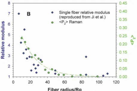
For amorphous and semicrystalline polymer systems, an increase in elastic modulus and strength can be attributed to improved chain orientation within the fiber with decreasing fiber size. For a deformation process, orientation is defined by two competing parameters: extensional forces and orientation relaxation. The first induces the orientation of polymer chains along the direction of deformation and the latter, because of the entropic cost associated with extending chains past their equilibrium coil dimensions, tends to return the polymer chains to their isotropic state.78 In the straight part of the traveling jet, chain orientation is high. Yet, bending instability that forces the jet to go into the looping trajectory has a significant influence on orientation and microstructure of the resulting fibers. It is however hard to estimate since the whipping motion is very rapid and has a large amplitude.82 A strong correlation between the modulus and the molecular orientation has been reported recently by our group for the polystyrene (PS) system at the single fiber level (figure 1.9).83

Figure 1.8 Generalized dependence of

Young’s modulus, strength and toughness on fiber diameter.

(38)

23

Chain organization in oriented fibers has been described by various models, such as the formation of confined supramolecular structures. Nanoscale organization into core-shell microstructure was also proposed, where the oriented chains would be located either in the core or in the shell of the fiber.81, 84 Camposeo et al.85 correlated the mechanical properties of electrospun fibers to their internal nanostructure and the core-shell organization. The preparation of fiber involves fast axial stretching of the polymer solution accompanied by radial contraction towards the core. As a result, the fibers display core-shell morphology with enhanced axial orientation at the fiber center. The fibers therefore have a much stiffer and denser core as compared to the shell. On the other hand, the study of poly(vinyl chloride) (PVC) electrospun fibers by Stachewicz et

al. has demonstrated improved mechanical properties of the oriented shell compared to

the isotropic core with much lower elastic modulus.86 Moreover, as the fiber diameter decreases, the volume fraction of the shell becomes more important, leading to a higher overall fiber elastic modulus.

Figure 1.9 Direct correlation between the diameter dependence of

(39)

24

Thermal properties

The electrospinning process has an effect on thermal properties of fibers, such as their crystallinity, crystallization temperature Tc, melting temperature Tm and glass transition temperature Tg. For instance, it has been shown that Tc increases for electrospun fibers in comparison to bulk samples for Nylon 11.87

The size dependence of properties of electrospun fibers has also been observed in thermal measurements, notably the change in glass transition temperature (Tg). Wang and Barber have investigated the Tg of electrospun poly(vinyl alcohol) (PVA) as a function of fiber diameter using indentation tests. They have observed a depression of Tg by 7 ºC with decreasing diameter from bulk values to the smallest diameter of about 100 nm. They have attributed this effect to polymer chain confinement within the fiber surface and amorphous regions within the fiber volume.88 On the other hand, the study of polyamide-6,6 by Baji et al. revealed an increase in Tg by around 7 ºC when the diameter of fibers decreased from micron size down to 200 nm. Higher values of Tg for the fibers with small diameters is caused by shear-induced molecular chain alignment during electrospinning, with smaller fibers experiencing higher draw ratios. Higher glass transition values also indicate better molecular coupling resulting in improved strength and stiffness.89 Yet, for PS systems, no changes in Tg were reported as a function of fiber diameter even though a large increase of shear modulus was observed.90

Thermal conductivity

A challenge with bulk polymeric materials is their inherent low thermal conductivity, on the order of 0.1 Wm-1K-1. As a consequence, it limits their use in many applications requiring this property.91 Electrospun fibers, due to the partial disentanglement and aligned and ordered molecular chains that result from high strain rates exerted on the liquid jet during the process, can be potentially used as materials with enhanced thermal conductivity compared to the bulk counterparts. However, a limited number of studies were performed on thermal conductivity of electrospun fibers. Recently, it was observed