MODELISATION ET OPTIMISATION DE
PANNEAUX RADIANTS HYDRONIQUES
Mémoire présenté
à la Faculté des études supérieures et postdoctorales de l'Université Laval dans le cadre du programme de maîtrise en génie mécanique
pour l'obtention du grade de Maître es sciences (M.Sc.)
DEPARTEMENT DE GENIE MECANIQUE FACULTÉ DES SCIENCES ET DE GÉNIE
UNIVERSITÉ LAVAL QUÉBEC
2012
Résumé
Ce mémoire présente la méthodologie et les résultats d'une étude numérique portant sur la modélisation et l'optimisation d'un système de chauffage par panneaux radiants hydroniques à faible masse thermique. L'objectif principal du projet est de fournir des données et de proposer des solutions au problème d'optimisation des performances énergétiques et du confort de tels systèmes. L'évolution du processus d'optimisation entrepris passe d'abord par une analyse détaillée de la modélisation du système, au terme de laquelle sont créés des modèles représentant la géométrie réelle des panneaux. Entre autres, un modèle semi-analytique est développé pour les panneaux avec configuration de tubes en serpentin et un modèle de volumes finis est développé pour les configurations de tubes en spirale. Les modèles choisis offrent la possibilité d'imposer des propriétés et des taux de transfert de chaleur non uniformes afin de représenter adéquatement la réalité lors d'un couplage avec l'environnement. Ces modèles servent ensuite à identifier l'effet de plusieurs paramètres de conception sur les performances énergétiques des panneaux radiants, d'abord dans un contexte découplé de l'environnement. Finalement, le problème complet du confort et de la demande énergétique de ces systèmes en climat hivernal québécois est traité dans la dernière partie du projet. Cette étape présente le couplage d'un modèle de dynamique des fluides numériques (DFN) avec le modèle semi-analytique de panneaux radiants pour tubes en serpentin développé préalablement. Le tout est intégré dans une pièce typique d'un bâtiment résidentiel afin d'analyser l'effet de la température d'entrée du fluide caloporteur ainsi que du positionnement et du dimensionnement des panneaux. Le modèle de DFN calcule les champs de vitesse de l'air, de température et de rayonnement dans la pièce pour fournir des valeurs locales du coefficient de transfert de chaleur au modèle de panneau radiant. Cette méthodologie permet de considérer le système de panneau radiant intégré à son environnement pour en optimiser les caractéristiques en regard du confort et de la performance énergétique.
Abstract
This master's thesis presents the methodology and results of a numerical study on the modeling and optimization of a hydronic radiant panel heating system with low thermal mass. The main goal of the project is to provide data and solutions to the problem of optimizing energy performances and comfort of such systems. The optimization process starts by a detailed analysis of the modeling task that yields models representing the real geometry of the panels. Among others, a semi-analytical model is developed for panels with serpentine tubing and a finite volume model is developed for panels with spiral tubing. The models chosen allow imposing non-uniform properties and heat transfer rates to correctly represent reality when the radiant system is coupled with its environment. These models are then used to identify the effect of numerous design parameters on the energy and comfort performances of the panels that are first modeled segregated from the environment. Finally, the complete comfort and energy consumption problem for winter conditions in the province of Quebec is addressed in the last part of the project. This step features the coupling of a computed fluid dynamic (CFD) model with the semi-analytical model for serpentine tubing previously developed. This is integrated to a typical room of a residential building to analyse the impact of the fluid inlet temperature as well as the position and dimensions of the radiant panels. The CFD model computes air speed, temperature and radiant intensity fields in the room to provide local values of heat transfer coefficient to the radiant panel model. This methodology allows considering the radiant system integrated in its environment to optimize its design parameters regarding the objectives of comfort and energy saving performances.
Avant-Propos
Les trois articles qui composent ce mémoire ont été coécrits par l'auteur du mémoire, Maxime Tye-Gingras, et son directeur de recherche, Louis Gosselin. Toutes les recherches, la confection des codes de programmation, la préparation des résultats ainsi que l'essentiel des textes des articles ont été réalisés par Maxime Tye-Gingras, qui en est l'auteur principal. Le travail de supervision dans le processus de recherche, de relecture et de correction des textes des articles a été assuré par le co-auteur Louis Gosselin.
Je tiens d'abord à remercier mon directeur de recherche Louis Gosselin, qui a su être à la fois un superviseur, un guide et un conseiller précieux dans la réalisation de ce projet. Mais surtout, déjà bien avant qu'aient été envisagées les premières lignes de ce mémoire, Louis a su me transmettre son enthousiasme et sa passion pour la recherche qui m'ont ouvert la voie vers la maîtrise.
De plus, les quelques heures de travail derrière cet ouvrage n'auraient certainement pas été les mêmes sans l'agréable compagnie de mes collègues de travail à qui je souhaite une carrière à la hauteur de leurs ambitions.
Finalement, je ne pourrais terminer sans remercier mes amis, mes proches, les membres des Harmoniques et de Com On Jazz, ainsi que ma famille et Caroline, ma douce moitié. Peut-être sans le savoir, tous ces gens qui ne liront sans doute jamais ce mémoire ont contribué indirectement à sa création.
Table des matières
Résumé ii Abstract iii Avant-Propos iv Remerciements v Table des matières vi Liste des figures viii Liste des tableaux ix Nomenclature x Chapitrel Introduction 1 1.1 Problématique 1 1.2 Objectifs 3 1.2.1 Objectif principal 3 1.2.2 Objectifs secondaires 3 1.3 Méthodologie et présentation du document 3
1.3.1 Chapitre 2 - Étude des hypothèses de modélisation du transfert de chaleur pour des panneaux radiants à configuration en serpentin destinés au chauffage et à
la climatisation 4 1.3.2 Chapitre 3 - Optimisation morphologique de panneaux radiants hydroniques 4
1.3.3 Chapitre 4 - Analyse du confort et de la charge de chauffage pour une pièce
avec plafonds et murs radiants hydroniques 5
Chapitre 2 Article #1 6
Abstract 7 2.1 Introduction 8
2.2 Semi-analytical radiant panel model 10 2.2.1 Step i) Initialize the temperature profiles 0f(x) and 6b(x) 14
2.2.2 Step ii) Calculate 5n (x) 15
2.2.3 Step iii) Solve the new temperature profiles 9f (%) and 0b (x) and iterate 16
2.2.4 Code verification 16 2.2.5 Physical interpretation of the tube layout in the models 16
2.3 Reference case for simulations 18 2.3.1 Overall panel heat transfer coefficient 18
2.3.2 Total linear thermal resistance R'tot 19
2.4 Results and discussion 20 2.4.1 Effect of the asymmetrical adiabatic condition on heat transfer 24
2.4.2 Effect of the ID conduction assumption 25 2.4.3 Effect of the semi-circular extremities 26
2.5 Impact of modeling assumptions for various geometries 2.6 Conclusions Chapitre 3 Article #2 27 29 31 Résumé 3.1 Introduction
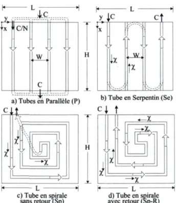
3.2 Description et modélisation du système 3.2.1 Modélisation générale
3.2.2 Tubes en parallèle (P) 3.2.3 Tube en serpentin (Sp)
3.2.4 Tube en spirale avec et sans retour (Sp et Sp-R) 3.3 Effet de la disposition des tubes sur la performance
3.3.1 Simulations
3.3.2 Détermination des facteurs d'influence
3.4 Effet des paramètres du système sur la performance 3.5 Conclusion Chapitre 4 Article #3 32 33 34 35 36 37 37 37 38 39 41 43 44 Abstract 45 4.1 Introduction 46 4.2 Description of the system 49
4.3 Modeling of the system 50 4.3.1 The coupled iterative procedure 50
4.3.2 CFD room modeling 51 4.3.3 Validation of the CFD model 54
4.3.4 Radiant panel modeling 55 4.3.5 Thermal comfort calculations 58 4.4 Thermal comfort and energy consumption results and discussion 60
4.4.1 Typical results for a specific case 60 4.4.2 Influence of the fluid inlet temperature, panel length and position 62
4.4.3 Influence of other parameters 65 4.5 Optimization of the system 66
4.5.1 Optimization procedure and Pareto analysis 66 4.5.2 Results and discussion of the multiobjective optimization 68
4.6 Conclusions 71 C h a p i t r e 5 Conclusion 72
Bibliographie 75 A n n e x e 78
Liste des figures
Figure 2.1 A schematic representation of the heating/cooling panel 11
Figure 2.2 A schematic representation of a panel slice 11 Figure 2.3 Representation of the asymmetry function 5 13 Figure 2.4 Iterative procedure of the semi-analytical model 14 Figure 2.5 Schematic representation of the models presented 17 Figure 2.6 Panel temperature field and cross section profiles with the semi-analytical
model for the reference case 21 Figure 2.7 Fluid temperature and efficiency distribution along the tube path 22
Figure 2.8 Non-dimensional asymmetry function for the reference case 23 Figure 2.9 Efficiency difference between the semi-analytical and analytical models 24
Figure 2.10 Frequency of occurrence of the error caused by the three assumptions for
various panel parameter combinations 29 Figure 3.1 Schéma des quatre configurations de tubes étudiées 34
Figure 3.2 Vue en coupe de l'assemblage tube-panneau et schéma des résistances
thermiques 35 Figure 3.3 Fréquence d'occurrence des écarts de performance relatifs pour
configurations Se, Sp et Sp-R 39 Figure 3.4 Probabilité normale de l'effet des variables pour les modèles Sp et Sp-R 40
Figure 3.5 Effet des paramètres de simulation sur le flux de chaleur moyen pour le
modèle P 42 Figure 4.1 Representation of the zone with one façade wall with a window and the
radiant panels on the ceiling and right wall 49 Figure 4.2 Schematic representation and stepwise description of the iterative resolution
procedure 51 Figure 4.3 Comparison of a) the horizontal temperature profile near the hot wall at
y = Hr/2 with TH = 29.3 °C and Tc = 10.9 °C , b) the vertical temperature
profile at x = Lr/2 with TH = 35.3 °C and Tc = 19.9 °C 55 Figure 4.4 Schematic representation of a serpentine hydronic radiant panel 55
Figure 4.5 Various temperature and comfort results obtained with a centered 2m long
ceiling panel 61 Figure 4.6 Schematic representation of the eight panel arrangements simulated 63
Figure 4.7 Influence of Tf,in on GDQ and Qô„t for the eight panel arrangements
simulated 64 Figure 4.8 Effect of mass flow rate change and fluid tube inlet permutation on the
GDQ and QU for the panel arrangements I and VI 66 Figure 4.9 Pareto fronts showing the trade-off between GDQ and Qôul for a) Lp^ot^m
and b) Lptot=2,4,6m 69
Figure 4.10 Combined Pareto front of all the designs tested for the optimal zone within
Liste des tableaux
Table 2.1 Panel parameters for the reference case 18 Table 2.2 Values of the varying parameters 27 Table 2.3 Models and methods used to measure the effect of the modeling assumptions 28
Tableau 3.1 Valeurs des paramètres de simulation 38
Table 4.1 Constant system parameters 50 Table 4.2 Panel and tubes constant parameters 56
Table 4.3 Constant comfort parameters applying throughout the study 59 Table 4.4 Parameters of the permutation and mass flow rate test simulations 65
Lettres latines
A Surface du panneau [ m2 ]
C Débit capacitif [ W / K ] D Diamètre [m]
E Effet d'un facteur [-]
F Coefficient de l'équation de transfert de chaleur [-] G Coefficient de l'équation de transfert de chaleur [-]
GDQ Cote d'insatisfaction globale (Global Dissatisfaction Quote) [%] H Longueur du panneau dans la direction x, Hauteur [m]
L Longueur du panneau dans la direction y, Longueur [m] N Nombre de rangées de tubes [-]
Nf Nombre de faces [-] Nel Nombre d'éléments [-]
PMV Vote moyen prédit (Predicted Mean Vote) [-]
PPD Pourcentage prédit d'insatisfaits (Predicted Percentage of Dissatisfied) [%] Q Taux de transfert de chaleur total [W]
Q' Taux de transfert de chaleur total par unité de profondeur [W/m] Q" Flux de chaleur moyen [W/m2]
R' Résistance thermique linéique [ m • K/W ]
R* Résistance thermique par unité de surface [ m2K/W ]
T Température [K]
T Température moyenne [K]
U Coefficient de transfert de chaleur global [ W/m2 K ]
W Distance des tubes [m] cp Chaleur spécifique [ J/kg • K ]
f Fréquence d'occurrence relative [-] k Conductivité thermique W/m K
h Coefficient de transfert de chaleur [ W/m2 K ]
m Coefficient de l'équation d'efficacité d'ailette [ m"1 ]
m Débit massique [ kg/s ]
m' Débit massique par unité de profondeur [ kg / s • m ] n Indice de la rangée de tube [-]
q Taux de transfert de chaleur [ W ]
q' Taux de transfert de chaleur linéique [ W/m ] q* Flux de chaleur [ W/m2 ]
r Rayon du tube [m] t Épaisseur du panneau [m] v Vitesse de l'air [ m/s ]
x,y,z Coordonnées cartésiennes [m]
Lettres grecques
r
Température adimensionnelle [-] A Différence [-] ô Décalage d'asymétrie [m] e Efficacité du panneau [-]n
Efficacité[-]0 Température relative T — Tref [K]
ë Différence de température moyenne T — Tref [K] P Densité de tubes [m- 1]
<P Ratio de températures [-]
<P Rapport dimensionel du panneau [-]
x,ç
Coordonnées locales [m]co Demi-espacement entre les tubes ( W - D„ )/2 [m] Indices A Analytique C Froid (cold) H Chaud (hot) S-A Semi-analytique a Air ambiant b Base de l'ailette
c Convection, contact, plafond (ceiling) f Fluide
fin Ailette (fin) h Convection i Intérieur in Entrée k Conduction
n Indice de la range de tube o Extérieur
opt Optimal
out Sortie, extérieur p Panneau
r Rayonnement, piece (room) rad Radiant
ref Référence
t Tube
tot Total w Mur (wall) win Fenêtre (window) x,y,z Direction x,y,z
Exposants
Introduction
1.1 Problématique
Les bâtiments sont de grands consommateurs d'énergie au Québec et on assiste, depuis quelques années, à un engouement pour les bâtiments verts. Les sources d'énergie alternatives ont la cote et leur utilisation de plus en plus répandue a un effet indéniablement bénéfique sur la trace écologique des bâtiments.
D'un autre côté, on ne saurait négliger l'impact du mode de chauffage et de climatisation sur la demande énergétique des bâtiments. En effet, une augmentation de l'efficacité des systèmes de chauffage et d'air climatisé (CAC) agit directement sur le problème en entraînant une baisse de demande énergétique à la source. De plus, un choix judicieux du système de chauffage et de climatisation permet de faciliter le couplage avec la source d'énergie préconisée et d'en tirer des rendements optimaux. Il semble donc logique de s'attaquer prioritairement à cette facette de l'énergétique du bâtiment en stimulant la recherche sur ces systèmes et en promouvant l'adoption de technologies de CAC éco-énergétiques.
Cependant, pour opérer un réel changement, il va sans dire que les solutions proposées devront offrir des avantages tangibles, tant au niveau économique qu'au niveau du contrôle et du confort des systèmes. Considérant cela, il importe de choisir une technologie qui :
i) Affiche un haut rendement énergétique
ii) Optimise le confort des occupants avec un contrôle approprié
iii)Est économiquement avantageuse (économies en énergie vs surcoût à l'investissement)
iii)Offre des possibilités intéressantes de couplage avec les sources d'énergie renouvelables présentes au Québec
Dans ce contexte, le présent mémoire traitera d'un type de système CAC innovateur émergent sur le marché : les surfaces radiantes hydroniques.
Les panneaux radiants hydroniques sont considérés comme une solution confortable, efficace et rentable [1] au problème de conditionnement thermique des bâtiments. Ils sont polyvalents et permettent le chauffage et la climatisation avec le même réseau de tuyauterie. Ils améliorent le contrôle thermique en découplant la tâche de ventilation de celle de chauffage et climatisation. De plus, grâce aux faibles différences de température requises, le système est particulièrement adapté pour être alimenté par des sources d'énergie renouvelables [2-3]. Finalement, tout dépendant du type de construction choisie, ils peuvent être utilisés dans une grande variété d'applications, du système à réponse rapide [4] jusqu'à la réduction de la pointe de consommation et au stockage énergétique par masses thermiques [5].
Cependant, en dépit du fait que de nombreux auteurs aient fait l'éloge du chauffage radiant hydronique, peu de données réelles ont pu appuyer les résultats théoriques avancés, et les études confirmant les avantages au niveau du confort sont toujours à attendre. Au contraire même, certains auteurs mettent en lumière les lacunes au niveau de la modélisation [5] et du contrôle des systèmes radiants [6] en déplorant les écarts importants de performances énergétiques entre les simulations numériques et les résultats expérimentaux.
On assiste donc manifestement à une situation où les modèles, les conditions de fonctionnement ainsi que les systèmes eux-mêmes doivent être améliorés pour atteindre les objectifs fixés d'économie d'énergie et de confort.
1.2 Objectifs
1.2.1 Objectif principal
L'objectif principal des recherches présentées dans ce mémoire est de donner des lignes directrices quant à la topologie et aux conditions optimales des systèmes radiants implantés dans des bâtiments résidentiels en climat québécois. Les objectifs d'optimisation de ce problème sont la minimisation de la demande énergétique et la maximisation du confort.
1.2.2 Objectifs secondaires
♦ Mettre au point des modèles mathématiques représentant la géométrie réelle des panneaux et les transferts thermiques impliqués dans le système. Implémenter et valider ces modèles dans un code de programmation afin de réaliser des simulations numériques.
♦ Analyser l'effet des divers paramètres du système dans un contexte d'application simple et optimiser les variables de conception qui influencent significativement la performance des systèmes de panneaux radiants.
♦ Optimiser le positionnement et les conditions d'opération des panneaux radiants dans une pièce typique afin de maximiser le confort des occupants et de minimiser la charge thermique du bâtiment. Cette tâche est accomplie en incorporant les modèles numériques développés et les résultats d'optimisation obtenus aux étapes antérieures dans un modèle de dynamique des fluides numérique récréant une pièce avec façade extérieure, soumise aux conditions hivernales québécoises.
1.3 Méthodologie et présentation du document
Les résultats des recherches présentées dans ce mémoire ont fait l'objet de trois articles soumis soit dans des revues avec comité de lecture, soit dans des conférences scientifiques. Les trois objectifs secondaires de la §1.2.2 sont donc adressés dans des articles distincts qui constituent les chapitres 2 à 4 du mémoire. Ces chapitres sont introduits et décrits
brièvement dans les §1.3.1 à 1.3.3 afin de mettre en évidence la continuité du processus de recherche à travers les trois articles.
Le projet repose entièrement sur des méthodes numériques, c'est-à-dire sur la construction et l'utilisation de modèles physiques-mathématiques pour évaluer les performances des systèmes étudiés. Les modèles sont validés au moyen de données trouvées dans la littérature et sont vérifiés entre eux par un traitement adéquat des hypothèses de modélisation. La revue de littérature associée au projet est présentée à l'intérieur même des articles, dans leurs introductions respectives.
1.3.1 Chapitre 2 - Étude des hypothèses de modélisation du transfert de chaleur pour des panneaux radiants à configuration en serpentin destinés au chauffage et à la climatisation
Cet article, qui a été déposé et accepté dans le journal Energy and Buildings, analyse quelques unes des hypothèses généralement utilisées dans la modélisation de panneaux radiants. En plus de présenter une revue de littérature des différents modèles existants, l'article expose trois méthodes de modélisation qui permettent de confirmer ou d'infirmer la validité des hypothèses discutées. Un modèle semi-analytique et un modèle de résolution par volumes finis, développés spécialement pour la recherche présentée, y sont décrits en détail. Les modèles sont tous implémentés sur le logiciel Matlab©.
Les travaux exposés dans cet article permettent de répondre au premier objectif secondaire de la §1.2.2, soit de développer numériquement et valider des modèles mathématiques reproduisant la géométrie réelle des panneaux. Concrètement, les conclusions de l'article ciblent les forces et les limites de chaque modèle en regard de la géométrie du panneau à modéliser. Ces modèles peuvent donc ensuite être utilisés dans les applications d'optimisation qui sont entreprises lors les étapes suivantes de la recherche. 1.3.2 Chapitre 3 - Optimisation morphologique de panneaux radiants
hydroniques
Cet article, qui a fait l'objet d'une conférence lors du Xeme Colloque Interuniversitaire Franco-Québécois sur la thermique des systèmes, présente une analyse de performance et une optimisation des paramètres géométriques et conditions d'opération des panneaux radiants hydroniques. Entre autres, l'étude fait appel aux trois modèles de panneaux
développés précédemment pour évaluer les performances de panneaux montrant diverses configurations de tubes.
Les résultats de cet article répondent au deuxième objectif secondaire de la §1.2.2 en isolant les paramètres de conception les plus influents et en les optimisant afin de maximiser le taux de transfert de chaleur des panneaux radiants. Ces conclusions sont utilisées pour déterminer une configuration de tube optimale, ainsi que les variables qui resteront enjeu lors de l'étape suivante d'optimisation, entreprise dans le dernier article du mémoire.
1.3.3 Chapitre 4 - Analyse du confort et de la charge de chauffage pour une pièce avec plafonds et murs radiants hydroniques
Cet article, soumis dans le journal Building and Environment présente le processus d'optimisation d'un ensemble de panneaux placés à l'intérieur d'une pièce d'une maison résidentielle typique en climat hivernal québécois. La méthodologie implique d'une part la résolution des équations liées à l'écoulement d'air et au champ de rayonnement dans la pièce par le logiciel de dynamique des fluides numérique (DFN) Fluent©. D'autre part, un couplage est effectué entre la DFN et un modèle de panneaux radiants développé préalablement. Le choix du modèle pour cette partie des recherches est basé sur les résultats de l'article précédent. Les résultats calculés par les deux paliers de simulation sont partagés mutuellement et itérativement réajustés afin d'obtenir la réponse du système complet de panneaux radiants dans son contexte réel. Le positionnement et la dimension des panneaux ainsi que la température de l'eau, identifiée comme variable d'influence dans l'article précédent, sont finalement optimisés pour maximiser le confort dans la pièce et minimiser la charge de chauffage.
Les résultats de cet article montrent la pertinence du travail d'optimisation et l'importance d'une modélisation du système tenant compte du contexte réel des surfaces radiantes. En d'autres mots, l'évaluation des performances d'un système radiant hydronique doit être faite en couplage avec l'environnement.
Article #1
Titre:
Investigation on heat transfer modeling assumptions for radiant panels with serpentine layout
Co-auteurs:
Maxime Tye-Gingras, Louis Gosselin Journal :
Abstract
This article aims at determining an optimal modeling method for heat transfer calculation of low thermal mass hydronic radiant cooling or heating panels with serpentine tube layout. It introduces a new semi-analytical procedure based on a well-known analytical modeling method to relax the thermal symmetry condition between tubes that is traditionally used. For the standard reference case presented, the temperature asymmetry was important, reaching 29% of the half inter-tube distance. However, the heat transfer performances were not significantly affected compared to results achieved by assuming thermal symmetry. It is also shown that this result implies that no significant performance gap between parallel layout and serpentine layout panels is expected. The effect of the ID heat conduction assumption and of straight tube endings in the modeling were also quantified using a 2D finite volume code. None of these assumptions caused significant errors on heat transfer calculations. The same results apply to a large range of panel geometries and operating parameters.
2.1 Introduction
Hydronic radiant heating and cooling panels and floors are gaining in popularity in the last years. For many reasons, they are considered as an efficient way to deliver heat and cold to a zone while achieving a high level of comfort of its occupants [1]. They are versatile, allowing heating and cooling with the same piping network. Furthermore, many systems that rely on renewable energy such as solar and geothermal energy can easily provide low temperature water flows that are particularly suited for radiant heating and cooling [2][3]. Finally, depending on the type of construction chosen, they can be used in a wide range of applications, from fast response air conditioning [4] to peak load reduction with high thermal mass [5].
Different types of modeling approaches have been developed over the years either to size these systems or to evaluate their performance. A finite element model was developed in [7] to model a radiant heating floor and allowed to study the influence of pipe diameter, thickness, material, number, etc. Ref. [8] developed a semi-analytical 2D model to simulate heat transfer in radiant systems with non-negligible thermal mass. An algebraic model is proposed by [9] based on the NTU method well-known in heat exchanger design problems. In Ref. [10], a different and more empirical approach is derived using data collected from a university building with radiant cooling ceiling. Finally, ASHRAE proposes an analytical model [11] originally developed for solar collectors [12] to simulate heat transfer in metal ceiling panels with negligible thermal mass. Used, among others, by Jeong et al. [13-14], [15-16] for the cooling capacity calculations of radiant panels, the model performs heat balance on the panel which is considered as a collection of fin-like elements. A somehow similar method is used in Ref. [17] for the calculation of the averaged heat flux of a radiant ceiling panel in meandering and spiral configurations. Although the agreement with experimental data is fairly good, the model is not developed to give the temperature profile on the panel, which might be important for characterizing air self-driven flow patterns as well as comfort in the room.
Nevertheless, despite the wide range of models developed and although many authors [1],[18-19] have predicted energy savings with radiant systems compared to standard convective heating/cooling systems, few field studies actually confirm those predictions.
Ref. [20] made an extensive study of a radiant floor heating system compared with a forced air system in an experimental house, and reported slightly higher overall energy consumption for the radiant system. However, the vertical air temperature profiles were more uniform and the radiant asymmetry due to external radiation was more efficiently countered, giving more comfortable conditions. Ref. [5] collected energy consumptions data of an experimental house on 4 years and reported important discrepancies between experimental and numerical results obtained with energy simulation softwares. Ref. [4] showed that for a radiant and a convective heating systems to achieve an equal steady thermal comfort in the same period of time would require a 22% oversized convective system. On the other hand, Ref. [6] studied a typical large building equipped with radiant floors and found that the energy consumption would have been 30% lower with a conventional variable-air-volume system than with the as-built radiant cooling-variable air volume combination. The authors emphasized the importance of a good design and operation strategies for the radiant systems to outperform traditional systems.
Therefore, there is still a need for developing better designing tools for radiant panels by the thermal engineering community. This cannot be accomplished without highly accurate models that yield detailed results (i.e. a complete panel temperature and heat flux field) to be able to take into account the complexity and local effects of radiative heat transfer. The models should also be able to simulate the real tube layout in order to allow optimization of the many design variables of a radiant system. In addition, the models to be used for optimization of performance should solve fast and be conveniently coupled with building energy simulation software or even CFD software.
The analytical fin-model used by Jeong et al. in Refs. [13] and [14] shows a great simplicity and speed of calculation while offering the potential for detailed results. Although the authors only used it for the derivation of a mean panel temperature, this model has the potential to give the whole temperature profile on a panel, which is a prerequisite to further detailed radiation and convection modeling in a zone. This analytical model was developed for parallel flow tube layout, which allows the use of a thermal symmetry (adiabatic) condition between the tube rows. However, serpentine layouts are, for technical reasons (i.e. simplicity of piping network), often preferred to parallel tube layouts. A priori, using the same adiabatic symmetry condition for a serpentine layout panel would
be inaccurate. Thus, a more exact model is needed to quantify the impact of the thermal symmetry assumption on the heat transfer and either replace the fully analytical model or confirm its accuracy for serpentine layouts.
The present paper proposes a new semi-analytical modeling method developed for low thermal mass serpentine layout radiant panels. The model computes analytical solutions to the Fourier heat conduction equation into fin elements of variable length and applies it on a
ID discretized domain to simulate the real topology of the tube layout. The paper also investigates the consequences of neglecting semi-circular tube extremities of the serpentine layout as well as neglecting the longitudinal (i.e. parallel to the tubes) conduction in the panel. These two assumptions are used in the proposed model and will be verified with a finite volume model featuring 2D heat conduction. This paper thus aims at introducing a new model and discussing its validity and its relevance regarding the simplifying assumptions.
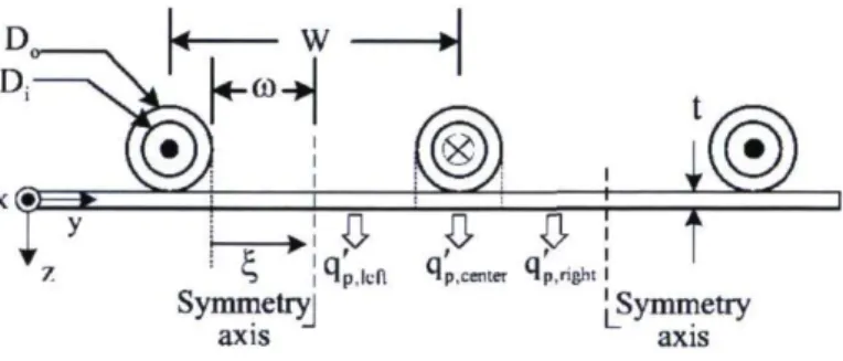
2.2 Semi-analytical radiant panel model
A cooling or heating panel with a typical serpentine tube layout is shown in Fig. 2.1. The tubing is in contact with a thin slab facing the zone and that acts as a heat spreader. Here, we considered panels with a negligible thermal mass, in such a way that a steady-state approach is sufficient. The fluid inlet temperature Tf,™ and zone air temperature Ta as well as the heat capacity rate of the fluid rhcp are known. The back of the panel (the insulated side) and the side walls of the panel are considered adiabatic. A Cartesian coordinate system (x,y) is used to express the absolute position on the panel. Its origin is located at the fluid inlet corner. A longitudinal coordinate system (x,Ç) is also used for calculations, with x following the tubing and Ç giving the inter-tube position (always in the positive y direction). The coordinates x and ^ are related to x and y with the variable n, the tube row index. Both systems of coordinates will be used throughout the development. For more details, see Fig. 2.1.
Isometric view Top view Fluid inlet -Inlet F ow direction -ft»
£
x r - W _ .m
Outlet-<r> vT
" v y \ \ ''-> . * ' n = f n = 2 n = 3 ' ••• \ \ • n - N <^ VFigure 2.1 A schematic representation of the heating/cooling panel
The model assumes no heat conduction in the x direction because the temperature gradient is supposed small compared to that in the y direction. This assumption will be later relaxed to quantify the effects of 2D conduction. As a first approximation, we also assume negligible effect of the semi-circular tube extremities (dashed lines on top view of Fig. 2.1), so the tubes are considered to be straight. The temperature at each tube row inlet is the same as that of the previous tube row outlet. This assumption will be later relaxed in a second analysis to consider the semi-circular extremities.
/ / <?
4p,lefl ^p,center Mp,right
m
Symmetry
L'-axis L'-axis Figure 2.2 A schematic representation of a panel slice
Without thermal loss (i.e. perfect insulation of the system), the energy balance over the base of a panel slice of thickness A%, as shown in Fig. 2.2, gives the following
qf = qp.left + qp.right + qP,center (2-1)
where qf is the heat transfer rate per unit length from the fluid to the tube base, and qP,ieft, qP,right, and qp>Center are the left, central (i.e., under the tube), and right part heat
transfer contributions per unit length from the base to the environment through the panel. Note that qp,ie« and qP,nghi will not be identical in the system considered. Assuming a total thermal linear resistance R'tot between the fluid and the base where the tube touches the panel, we have
, 0 f - 9b „
q f = - ^ 7 — (2-2) where 0 = T - T*. RL will be calculated later. The central part of the panel slice (under the
tube) is assumed to be at the base temperature 0b, so
qUnter = U D A (2.3) U is the overall heat transfer coefficient and will be derived later. The heat transfer per unit
length on the left and right parts of the panel slice are calculated with the fin equation for heat transfer rate assuming an adiabatic tip condition:
qén = UriftaLfinOb (2.4) where !"!&, is the fin efficiency and Lfin is the length of the fin considered. Lfin needs to be
determined for both the left and right sides of the panel slice. For a parallel tube layout, we have a symmetry (i.e. adiabatic) condition in the middle between each tube row, so
Lies = Lright = co, where co = ( W - D„ )/2 .
However, for a serpentine layout, this condition no longer holds. We thus define the asymmetry function 5n (x) as the displacement (positive along y) of the adiabatic line with respect to the geometrical inter-tube symmetry line at any coordinate x on the panel between the tube rows n and n+1. That is:
This is schematized in Fig. 2.3. We can now express the fin length of the left and right parts of a panel slice located at a coordinate x of the nth row as
Lieft,„(x) = © - ô „ - i ( x ) (2.6a)
Lright.n(x)=CO + Ôn(x) (2.2.6b) We will explain below how to calculate S .
Geometrical Symmetry axis
i
T:
S v X LM-fî
Adiabatic line n-ffi-w J. \■±
Using Eqs. (2.1) to (2.2.4) combined with the temperature raise of the fluid due to sensible heat transfer through the panel slice gives the total energy balance equation of a panel slice:
dOf 0f qr = C
-dX R(ot(l + l/F)
with
F = R'totU [r|leftLleft + n.rightLright + D0J
and tanh(mLieft) tanh(mLright) rjieft = qright = mLieft mLright m
-VÛ/kt
(2.7) (2.8) (2.9) where n, is the fin efficiency of the panel slice and C is the heat capacity rate (rhcp). The right hand side equality of Eq. (2.7) is a one-variable first order differential equation (D.E.) that can be solved for 0f (x) with a boundary condition 0f (0) = 0fjin to get the total heat transfer rate of the panel. If tube spacing is uniform and thermal symmetry between tubes is achieved, as in parallel flow panels, the overall non-dimensional panel slice efficiency F isa constant and the integration is straightforward to obtain a simple analytical solution. However, in serpentine layout systems, F is likely to be a non trivial function of x, so the D.E. needs to be solved numerically by discretizing the tubing longitudinally in many elements (i.e. slices) of thickness Ax- However, 5„(x), and thus F(x), cannot be calculated without the prior knowledge of fluid temperature distribution, since this is required to calculate the panel temperature profile and locate the adiabatic line (i.e. the positions where ô9p/ôi; = 0 for each discrete value of y). A general iterative procedure is thus developed and shown in Fig. 2.4. Each step of the procedure will be described in more details in the next sub-sections.
(i) Initialize the fluid and tube base temperature profile along X for the whole tube length with the analytical expression assuming centered symmetry.
i
EqMlOHU)(ii) Compute the temperature between each row of tubes using the fin equation with prescribed
boundary temperature. Then solve to find the extremum with respect to ^ and calculate 5n ( x ). | ^s"' ' * '
(iii) Solve the D.E. numerically for the new fluid temperature profile. Eq. (7) Figure 2.4 Iterative procedure of the semi-analytical model 2.2.1 Step i) Initialize the temperature profiles 9f(x) and 6b(x)
With the symmetry assumption, 5 = 0 everywhere, F is a constant and Eq. (2.7) is solved analytically for Of (x) • Then, using Eq. (2.2) and the left hand side equality of Eq. (2.7), we can find the tube base temperature distribution 9b (x) • The procedure is detailed in [14], so only the result is shown here:
Qf ( x ) = Qf.» exp -WUG with G = 9b(x) = ef(x)(l-WGURU) 1/U (2.10) (2.11) tanh(mft>) W U [ D0+ r i ( W - D0) ] + R ; tot mco
Even if we assume thermal symmetry, these equations are only valid upon the assumption that the coefficient -WUG/C is a constant, which is the case in the present study. However, even though the thermal resistance R!0,, the tube diameter D0 and the heat capacity rate are not subject to important variations in the direction x, the tube spacing W, the heat transfer coefficient U and the fin efficiency r\ may do so. This reinforces the relevance of a numerical resolution of the D.E. of Eq. (2.7), as used in the proposed semi-analytical model. In the cases where the parameters are not uniform, the semi-analytical model cannot provide an initial guess for the fluid and base temperature. One should thus make an initial guess on the Sn (x) function and start the iterative procedure at step iii) as explained in §2.2.3.
2.2.2 Step ii) Calculate ô„ (x)
Knowing 0b (x)> one should first discretize the domain in slices of thickness Ax, and make the change of coordinates to get 0b n( x ) . Then, for given x and n (with 1 < n < N - 1 ), the panel slice temperature profile with respect to the £, -coordinate between two consecutive rows of tubes (excluding the part under the tube) is given by the fin equation with prescribed temperature boundary condition [21]:
9P>„ (£,x) _ (pb,n (x)sinhm^ + sinhm(2où-£,) 9b,„(x) sinh2mco where <k,n (x) = 9b,„+i (x)/9b,n(x).
We can compute the gradient with respect to \ and solve for d9p/d£, = 0 to find the position of the temperature extremum. The solution is given by
f v—, ;—77 ; — A ^U/a-o m ta
V-(*-e-
2m<°)(<p-e
2nKÛ)
(2.13) (<p-e ) v v ' JThe value of £| ._ has physical interpretation (i.e. ranges within 0 < El ,~ A 2co) only if
— i = — ' - < § y J- (2.i4)
l + ( e2- )2 2
Finally, we recall Eq. (2.5) to find 5 and apply this procedure on every panel slice of thickness Ax to get the whole ôn(x) profile for n = l to N - l . By assumption, 5n=o(x)
and Ô„=N (x) are equal to zero, because of the adiabatic condition imposed on the extreme
left and right boundaries which correspond to the side of the panel.
2.2.3 Step iii) Solve the new temperature profiles 0f (/) and 6b (/) and iterate
Knowing 8n(x), Eq. (2.7) can now be solved numerically for q'(x) and 0f (x)with a forward finite difference scheme, starting from the tube inlet, where the fluid temperature is known. The base temperature profile 0b (x) is then directly calculated by
eb(x) = o,(x)-Ri-q'f(x) (215)
Steps (ii) and (iii) should be repeated as long as the 8„(x) function keeps changing significantly from an iteration to another. Convergence is declared when the maximum local value of the relative difference on ô„ (x) between two consecutive iterations drops under 0.1%.
2.2.4 Code verification
The verification of our code was performed by comparing the fluid temperature distribution of the analytical model of Eq. (2.10) to that of the proposed model for which we imposed 8n (x) = 0 everywhere. For the reference case (see next section) the results yielded by both models were identical with discrepancies under 0.01%.
2.2.5 Physical interpretation of the tube layout in the models
The physical interpretation of the various models that will be discussed in this paper and their assumptions is more easily understood with visual representations. This section aims at clarifying the modeling variations seen so far. First, Fig. 2.5a is the schematic representation of the semi-analytic model described in the last section. It is a serpentine with straight tube ends.
The second one, shown in Fig. 2.5b, is the analytical model used by Jeong et al. [14], that was developed for parallel flow layouts comprising N tubes of length H, each one having a specific heat capacity rate of C/N (i.e. the total specific heat capacity rate is C). In that case, the fluid temperature in each tube at a position x is given by [14]:
Mx) = ef,inexP where 0f is solved from x = 0 to x = H .
f-NWUG x
Jî
H *<\ \ 7L
5C
. w
<A \ 7X
.n
C/N . K J K - . .a) Serpentine layout: semi-analytical model 111
-Je
b) Parallel layout: analytical model Eq. (16)
%
i
^ =»= ^>=
T
w
_L
NxH
c) "Unrolled" layout: analytical model Eq. (10) Figure 2.5 Schematic representation of the models presented
In the present study, however, we used a slightly different version of this analytical model because serpentine layout was considered. In Eq. (2.10), the total heat capacity rate C appears rather than C/N in Eq. (2.16) because in the serpentine layout, the flow is not divided in N. We must then solve 0f from x = 0 to % = NH with the heat capacity rate C. When the thermal symmetry assumption is invoked (i.e. 5 = 0), this is equivalent to unrolling the tube of Fig. 2.1 and attaching it on a single strip panel. This is shown in Fig. 2.5c.
Despite the fundamental physical difference between Fig. 2.5b and Fig. 2.5c, it can be shown that both yield the same total heat transfer rate. Assuming no loss, the total heat transfer rate is given by:
q.ot=C(0f,in-Of,out) (2.17)
where Gf.ct is taken at x = N x H in Eq. (2.2.10) and at x = H in Eq. (2.2.16). Taking the same values of C, T^n, and WUG, both equations give the same fluid outlet temperature Gf.out, and the total heat transfer is the same. In other words, if one can show that the
symmetry assumption provides precise temperature output for a serpentine layout panel, then the serpentine and parallel layouts have equivalent thermal performance.
In practice, the value of the non-dimensional coefficient G will be slightly affected by the variation of the flow rate (i.e. C/N instead of C) from one model to another because it influences the convection resistance of the fluid inside the tubes.
2.3 Reference case for simulations
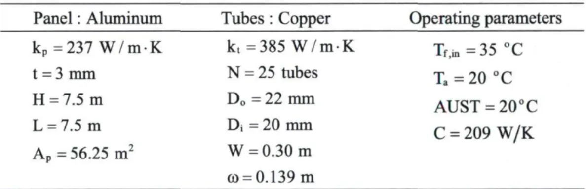
The simulations results that will be presented in the next sections are based on a reference case. Note that the choice of the different system and operation parameters is somewhat arbitrary, since the model is built in a very general fashion to ensure its versatility. Other parameters will be considered in §2.5. We consider a heating hydronic radiant ceiling panel with a serpentine tube layout, as shown on Fig. 2.1. The parameters used for the reference case are summarized in Table 2.1.
Table 2.1 Panel parameters for the reference case
Panel : Aluminum Tubes : Copper Operating parameters kp= 2 3 7 W / m - K k, =385W/m-K Tf,m=35°C t = 3 mm N = 25 tubes j = 20 °C H = 7.5 m Do =22 mm AUST = 20°C L = 7.5 m Di = 20 mm Ap= 56.25 m2 W = 0.30m co = 0.139m C = 209 W/K
2.3.1 Overall panel heat transfer coefficient
Many studies have been performed to determine the convective and radiative heat transfer coefficients over heated or cooled surfaces in enclosures such as rooms. A review presenting the work done in this field before 2001 is available in the literature [22]. The large amount of more recent publications [23-26] related to this subject shows the complexity of such a task. It is not the purpose of this article to discuss the various methods and correlations available in the literature. Therefore, the procedure presented below to determine the overall heat transfer coefficient of the panel U will be kept as simple as
possible, since the model presented implies no specific method. Indeed, almost any procedure for the calculation of U could be embedded easily in the model described in §2.2, even if U varied with temperature and with position.
For convenient calculations, we assume AUST = Ta, where AUST is the area-weighted temperature of the indoor surfaces excluding the panel and Ta is the air temperature, assumed uniform in the room. The natural convection coefficient hc,p on the surface of the panel in the reference case is assumed to be uniform and is calculated with the correlation of Min et al. for a heating panel [27], as suggested by ASHRAE [11]:
hc>p=0.134(Tp-Ta)°25 (2.18)
where Tp is the averaged temperature of the panel. The radiation coefficient hr,p is calculated with the following equation [11]:
hr,p=5xlO"8[AUSTATp2]-[AUST + Tp] (2.19) Tp is related to U and to the total fluid temperature drop in the following way:
qtot = C (Tf,in - Tf,ou« ) = ApU0p (2.20)
where Ap is the area of the panel. When AUST = Ta, U = hc,p +hr,„. U is found with an iterative procedure, first using Eq. (2.7) to find the outlet fluid temperature Tf,out, then finding Tp with Eq. (2.2.20), and finally computing a new value for U using Eqs. (2.2.18) and (2.2.19).
The model of §2.2 could also use a non-uniform panel heat transfer coefficient. Actually, the analytical solution for each individual fin is based on a uniform heat transfer coefficient condition, but each fin element can be assigned a different value for U, which is a considerable advantage for coupling the model with CFD simulations where local effects from radiation or even natural or mixed convection can be taken into account.
2.3.2 Total linear thermal resistance R'tot
The total linear thermal resistance incorporates the inner tube fluid convection resistance RJ,, the tube conduction resistance RL and the contact resistance between the tube and the panel Ré :
R'to, = R U R k + R é (2.21) The two former resistances are given by [21]:
RL= * R ^ - - l M ) (2.22)
27n\hf 2îikt
where the internal heat transfer coefficient hf is determined by the pipe dimensions and the flow rate, using an appropriate correlation that can be found in literature [21]. The contact resistance for different types of tubing attachment is given in [11]. We will consider copper tubes secured to an aluminum sheet with welding. The linear thermal resistance values yielded for the reference case are thus:
Rh=0.02 RL=4xl0"5*0 R:=O.I2
R;O, =0.14m-K/W
Rk is negligible compared with the other resistances.
2.4 Results and discussion
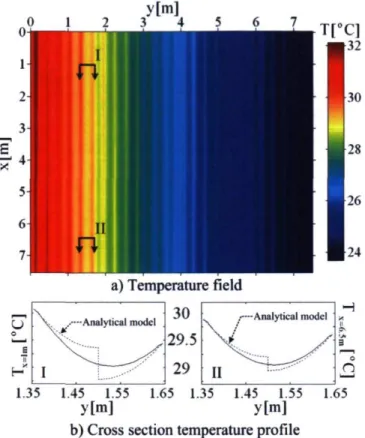
A simulation of the reference case is performed with the proposed semi-analytical model to relax the assumption of symmetrical adiabatic line between tubes. The code used for programming the model is a Matlab routine. We discretized the domain in Nelx =100 elements in the x-direction. With N = 25 tube rows, that makes a total of N x Nelx = 2500 fin elements along the tube path x- This discretization has been chosen so that doubling the number of elements yielded a difference under 0.01% on the total heat transfer rate qtot. Since the temperature distribution of the panel along each fin element is evaluated analytically, the precision of the result is not affected by the choice of a mesh size in the y-direction. Typically, the model needs 7 iterations for the 8n(x) function to reach convergence
Figure 2.6a) shows the panel temperature field generated by the model, and Figure 2.6b) presents the cross section temperature profile at x = 1 m and x = 6.5 m between the 5th and the 6th tube row to show the progression of the temperature asymmetry along a row. These profiles are compared with the ones obtained with the analytical model (in dashed lines), relying on thermal symmetry. It is interesting to note the temperature gap in
the panel at the position corresponding to the mid-distance between tubes, for the latter, while the temperature profile is smooth with the proposed methodology.
1.35 1.45 1.55
y[m] 1.65 1.35 1.45 1.55 y[m] 1.65 b) Cross section temperature profile
Figure 2.6 Panel temperature field and cross section profiles with the semi-analytical model for the reference case
The nearly ID profile seen in Fig. 2.6a) confirms that the panel temperature gradients are considerably more important in the y direction than in the x direction, as predicted earlier. In that situation, the simplification to a ID model seems possible, but before, one should analyze the two types of gradients observed along y. The first type is the local gradient pattern, present between each tube row due to the fin effect, which is described by a ID equation and would thus be appropriately used in a ID model. The second one is the overall panel gradient (i.e. the drop from 32oC to 24oC from left to right on Fig. 2.6a) and is due to the continuous fluid temperature drop along the serpentine. Remembering that this drop occurs according to the coordinate x, parallel to x, the overall gradient in y observed is thus indissociable from the gradient in x. One can thus question the physical signification and the feasibility of a ID model. Nevertheless, for some applications where a ID profile is required (e.g. CFD heat transfer modeling in a 2D room), Fig. 2.6 shows that an x-averaged profile or a profile taking a slice (at H/2 for example) could be used without much error.
However, care should be taken in that case, because using a high fluid inlet temperature, a low heat capacity rate and a low number of tube rows would make the gradient in x more significant. The ID model would then be practically irrelevant.
The model achieves a good speed of calculation by generating the temperature profile of Fig. 2.6a in 0.3 second on an Intel Xeon CPU 5150 @ 2.67GHz for a
(Nelx = 100)x(Nely = 800) grid. This feature would be particularly useful for coupling the model with a 3D room CFD simulation, where each node of the heating/cooling surface must be assigned a specific temperature.
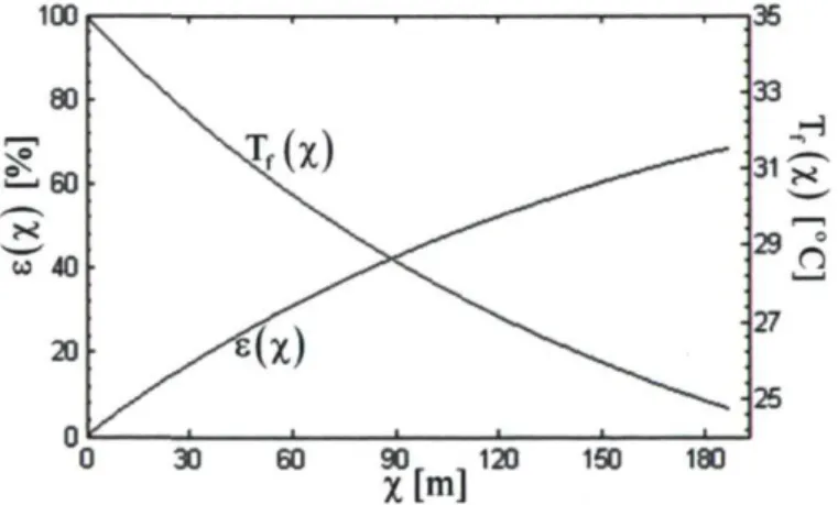
The heat transfer performance from the fluid to the environment is now measured by using an efficiency parameter evaluated at each position x along the tube, in a similar way as in heat exchanger theory:
q ( x ) _ Tf, ,n- Tf( x ) _ 9 f ,i n- 9f( x )
Qmax
■ ( % ) (2.23)
Tf,in — Ta 9fjin
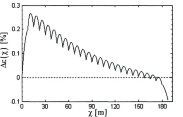
Fig. 2.7 shows the efficiency and fluid temperature profiles along the tube. The total efficiency of the system is approximately 68% with a fluid temperature drop of 10°C and the total averaged heat flux is q"ot = 38.128 W/m2.
30 60 90r , 120 150 180
X[m]
Figure 2.7 Fluid temperature and efficiency distribution along the tube path
Due to the negative exponential trend of the efficiency function (i.e. diminishing return), reaching a fairly higher efficiency value would necessitate a huge increase in the panel area and the total tube length. Actually, with its asymptotical behavior, an efficiency of 100% would be reached only with an infinitely long tube. In design applications, higher total heat transfer rates can be achieved by using many smaller panels reaching lower total
efficiencies. In that context, the efficiency function can be a useful tool in optimization tasks to determine at which point the addition of a new panel is beneficial regarding cost and heating/cooling requirement constraints. In the present case, however, a deliberately high exchange length and panel area have been chosen to show the shape of the efficiency function, but no performance optimization is attempted in this article.
Another interesting result is the S„(x) distribution that is shown in Fig. 2.8, where ôn(x) = ô„(x)/(o is the non-dimensional asymmetry function for the nth tube. The graph shows only the 8-profile from n = 4 to N - 4 , for which all the 8n(x) are identical (or nearly identical so that they cannot be distinguished in Fig. 2.8), but alternatively up and down from a tube row to another. The values of ô„(x) for the first and last rows are slightly lower due to the imposed boundary condition 50(x) = 8N(x) = O V x . A s it can be observed on the figure, the function shows a linear behavior (i.e. 8n(x)ocx) with a regression coefficient of R2 = 1. 0.24 0.20 ^£
2
0.16
0.12 0.08 U 1 2x[m]
Figure 2.8 Non-dimensional asymmetry function for the reference case
It appears clearly from Fig. 2.8 that the symmetrical adiabatic condition is not achieved, because the real adiabatic line deviates up to 24% away from the symmetry axis in some areas of the panel.
Note that a local deviation of more than 100% would mean that the solution to Eq. (2.13) does not respect the condition of Eq. (2.14), because the zero-gradient point for temperature would be outside the calculation domain of the inter-tube fin. Such a case would make the proposed modeling unusable but is generally unlikely to occur, because that would be the consequence of a non-optimized design. Indeed, it would mean that some
sn = 5,7...21
■
■
/ f f = 4 , 6 . . . 2 0
heat is transferred from a tube to another instead of being dissipated in the environment, which is obviously not desired.
2.4.1 Effect of the asymmetrical adiabatic condition on heat transfer
It has been shown in the last sub-section that for a standard design, the thermal symmetry condition is not observed. A priori, it would mean that the analytical model is not suitable for calculations that imply serpentine layout tubing. However, simulations show that the adiabatic line displacement has only a weak incidence on the total heat transfer rate from the fluid to the panel. Comparing the panel efficiency profiles of the semi-analytical (i.e. considering thermal asymmetry between tubes) and analytical models (i.e. considering symmetry) yields surprisingly similar results. Fig. 2.9 reports the efficiency gap between the two models:
Ae(x) = e(x)s_A-e(x) (2.24)
where the subscripts S-A and A refer to the semi-analytical and analytical models respectively. The absolute value of efficiency difference observed at the outlet ˣout (and thus the total heat transfer difference) is under 0.1%, which is of the same order of magnitude as the semi-analytical model precision. Besides that, the maximum deviation of 0.3% exhibited in Fig. 2.9 shows that the adiabatic symmetry assumption is verified on any point of the panel for heat transfer calculation purposes in the reference case presented.
0 30 60 90 120 150 180
X[m]
Figure 2.9 Efficiency difference between the semi-analytical and analytical models
This trend can also be verified in the limit for which Max(8n(x))«l. It can be achieved with a system where L = 3m, H = 1 8 m , N = 15 tubes and W = 0,20 m and all the other parameters are the same as in the reference case. For that design, the simulation
yields Max(8n(x)) = 0.955, Aeout=-0.7% and Max(As(x)) = 1.8%. The error is relatively high compared to the previous cases, but is still negligible when considering the uncertainties on the design parameters and on the actual panel heat transfer coefficient. Moreover, one should keep in mind that this latter design is an extreme case that will rarely be encountered in practice. It is therefore clear that the thermal symmetry assumption is valid when calculating the heat transfer rate.
The last conclusion has an important implication concerning the choice between parallel or serpentine layout in a design process. Practically, Aeout gives the performance gap between a serpentine layout panel and its "unrolled" layout panel (see §2.2.5 and Fig. 2.5). On the other hand, it has been shown that the total heat transfer rate of a parallel layout panel is equivalent to the one achieved by the "unrolled" panel. The negative value of Aeout thus means that real serpentines will actually lead to slightly lower heat transfer rates, as it is commonly believed. However, the performance reduction is not significant and thus the choice of one or the other in an engineering application should be based on technical and economical considerations first rather than heat transfer performances.
2.4.2 Effect of the ID conduction assumption
Both the analytical and the semi-analytical models assume that the heat conduction is negligible in the x-direction due to low temperature gradients in the panel. The procedure presented in this section aims at relaxing this assumption to quantify its effect on the heat transfer rate. A finite volume code is used to implement 2D conduction in the panel with convection on its surface area. The fluid tubes are represented as source lines located on the sides of the appropriate cells located "under" the tubing. The power dissipated by the local source line is linked to the local fluid temperature and to the panel temperature of the neighboring cells. The fluid temperature distribution and the panel temperature profile update iteratively until the solution is stabilized. The mesh is made of uniform rectangular cells with (Nelx =400)x(Nely =800) and all the boundaries of the domain are adiabatic. The convergence is considered to be reached when the residual normalized by the number of cells drops under IO"8.
The code was verified by imposing the conductivity in the x-direction to be null and comparing with the semi-analytical model for the reference case described in §2.3. However, due to the type of modeling chosen (i.e. source lines for the fluid heat input), the
tube outside diameter must be set to D0 -> 0. The two models yield similar results with less than 0.01% discrepancy, which verifies the 2D finite volume code.
The conductivity is then set to kx =ky = 237W/mK and the heat transfer efficiency function e(x) is compared to that of the semi-analytical model. Although the comparison of the temperature field of the panel gives local variations of up to 1% between the two models, the efficiency function is the same with, again, less than 0.01% of discrepancy. This result proves that the conduction in the x-direction is negligible and that the ID conduction fin approach used in the analytical and semi-analytical models is sufficient.
To conclude this section, it is worth mentioning that the 2D finite volume code used for the verification of ID conduction assumption would not be an appropriate tool for modeling heat transfer in hydronic radiant panels because it is very expensive computationally (calculations took more than 2 minutes).
2.4.3 Effect of the semi-circular extremities
The real topology of serpentine layout radiant panels comprises semi-circular links between each tube row. The impact of this feature on the heat transfer should be characterized in order to validate or bring a correction to the proposed model. For this task, the 2D finite volume model is used with a special mapping of the source line mesh frontiers to simulate the real tube path. Due to the regular rectangular mesh used, the total effective length of tubing in the semi-circular parts must be adjusted to fit that of a real circle. This is because the use of orthogonal segments to approximate a semi-circular path gives a tube segment length of 2W instead of rcW/2.
Although it has been shown previously that ID conduction is sufficient in the case of straight tubing modeling, conduction is enabled in both directions because it may have a significant effect with the presence of semi-circular endings. The system parameters and conditions of operation are given in the reference case of §2.3, except that the tube diameter is again neglected. The mesh is (Nel* = 400)x (Nely = 800), as in the previous section.
In practice, the inner tube fluid convection resistance RJ, may decrease in the curved sections of the tubes. However, this is neglected since this resistance accounts only for a small part of the total thermal resistance, as seen in §2.3.2. For example, doubling the inner tube convection heat transfer on the whole tube length yields a total heat transfer rate only
0.7% higher than for the reference case. This phenomenon might however be more important in laminar flow applications, where RÎ, is sensibly higher, which is not the case in this study.
The total averaged heat flux is compared with the one obtained with the semi-analytical model to evaluate the effect of the semi-circular extremities. The results indicate that despite the somewhat important topology modification made by considering this feature, the two cases yield again very similar total heat transfer performances with only 0.1% of difference. It is thus clear that the semi-circular extremities can be neglected in the heat transfer analysis and straight tube modeling is sufficient for heat transfer calculations.
2.5 Impact of modeling assumptions for various geometries
In the previous section, the assumptions used in the heat transfer calculations of serpentine layout panels have been verified for the reference case (see §2.3). In order to generalize the conclusions of this paper, the following section presents a summary of the same verification process for various panel geometries and operating parameters.
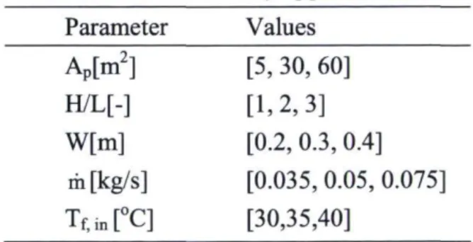
We let five parameters vary: the panel surface area Ap, the panel aspect ratio H/L, the inter-tube distance W, the mass flow rate rb, and the fluid inlet temperature Tf, ;n. All the other parameters are kept the same as in the reference case of §2.3. Each varying parameter is allowed to take three values that are given in Table 2.2.
Table 2.2 Values of the varying parameters Parameter Values AP[m2] [5, 30, 60] H/L[-] [1,2,3] W[m] [0.2, 9.3, 9.4] m[kg/s] [9.935, 9.95, 9.975] Tf,in[°C] [39,35,49]
The extreme values of the parameters are chosen to test a large span of possible cases, but making sure that the maximum value of the non-dimensional asymmetry function 8 always remains under 199%. This allows using the semi-analytical model for every case
tested. The minimum value of the mass flow rate m is also chosen so that the flow regime in the tubes remains turbulent. This way, the inner tube fluid convection linear resistance Rh does not vary significantly compared with the total resistance R',0t. We thus consider that Riot keeps the same value as in the reference case.
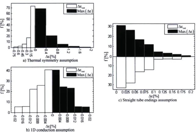
Each possible combination is tested, which makes a total of 35 = 243 different cases. For each of the parameters combination, the effect of the thermal symmetry assumption, the
ID conduction assumption, and the straight tube ending assumption are verified, as presented in §2.4.1, 2.4.2 and 2.4.3 respectively. The effect of each assumption is measured by comparing the efficiency function of two models and taking its maximum difference (i.e. Max(Ae)) as well as its difference at the outlet (i.e. A£out). Table 2.3 summarizes the models and the methods used for measuring the effect of each assumption on heat transfer rate calculations. Figure 2.19 presents the results in histograms giving the relative frequency of occurrence f among the 243 cases tested in each range of error achieved. For example, if 37 cases tested fall between 9 and 9.25% of error, then
fo-o.25%=37/243 = 15.2%.
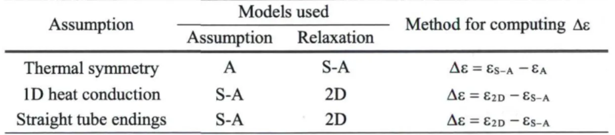
Table 2.3 Models and methods used to measure the effect of the modeling assumptions
Assumption Models used Method for computing Ae Assumption
Assumption Relaxation Method for computing Ae Thermal symmetry A S-A Ae = SS-A — £A
ID heat conduction S-A 2D A s = £2D - £S-A
Straight tube endings S-A 2D A S = E2D - ES-A
A= Analytical model, S-A= Semi-analytical model, 2D= 2D finite volume model
The results obtained allow generalizing the conclusions stated for the reference case in §2.4. Using the thermal symmetry assumption for serpentine panels has the effect of slightly overestimating the total heat transfer rate. At the opposite, considering straight tube endings instead of semi-circular endings has the effect of underestimating heat transfer. The ID conduction assumption has virtually no effect. In every case, none of the assumptions caused errors of more than 2% on the heat transfer rate of serpentine radiant panels. The conclusions of the last section thus hold for a large range of panel geometries and operating conditions.
70 60 I lAeM ■ ■ M a x (Ac) . - , 5 0 ■ 30 ■ 20 e— M H 10 0
^ = E =
6 6 6 6 6 ° P g C, £ M fe CD w * 09 AE[%]a) Thermal symmetry assumption
0 0.025 005 0.075 0 1 0.125 0.15 0 175 0.2 Ae[%]
c) Straight tube endings assumption
6 6 6 6 6 ° P P P P °
S
f 2 § | § § g g S
AeJ%]
b) ID conduction assumption
Figure 2.10 Frequency of occurrence of the error caused by the three assumptions for various panel parameter combinations
2.6 Conclusions
The purpose of this paper was to consolidate the foundations of serpentine layout hydronic radiant panel heat transfer calculations by bringing confidence into the modeling assumptions that are commonly used. For this task, we introduced a novel semi-analytical numerical model for computing steady-state heat transfer and temperature field of such panels. It proved to solve fast and to yield detailed heat transfer rates and temperature fields over a heating or cooling surface. The model was compared to a fully analytical one recommended by ASHRAE and well detailed in [14]. A comparative study was conducted to evaluate the impact of relaxing the symmetrical adiabatic condition between the tubes for the serpentine layout. The paper also quantified the effect of the ID heat conduction assumption used in both the analytical and semi-analytical models by comparing the result with a 2D finite volume code computing the full temperature field of the panel. Finally, the semi-circular extremities linking the tube rows together were modeled in detail with the
finite volume code and the results were compared with the ones of the semi-analytical model assuming straight endings.
The main conclusions of this study are that, for a large range of panel geometries and operating parameters, all the assumptions used yield negligible errors on heat transfer of a radiant panel. Thus the analytical analysis is sufficient in the case of serpentine layouts, as it is for parallel ones. Some other conclusions can also be drawn from that work:
- The 2D finite volume model is versatile but uselessly heavy. Indeed, it can reproduce any tube pattern, but it is very slow to converge because it uses an iterative numerical resolution scheme instead of relying on analytical solutions. Furthermore, it relaxes the ID conduction and the straight tube endings assumptions but these proved to yield no significant error. However, it is a good tool for the verification of simpler models.
- The analytical model is fast and accurate, but not very versatile since the tube spacing, the heat transfer coefficient and the fin efficiency must be constant over all the tubing length for the methodology to be applicable.
- The semi-analytical model is versatile, fast and accurate, but the iterative methodology to find the 8„ (x) function is not required for standard heat transfer calculations in serpentine panels. The numerical finite difference scheme used in the semi-analytical model is efficient and allows solving the D.E. for the fluid temperature profile with non constant parameters. It thus offers good potential for coupling with CFD simulation programs for detailed convection and radiation calculations. Other simplified models taking advantage of the almost ID nature of the temperature profile in Fig. 2.6 could also be developed to be coupled with CFD programs by post-treatment of the results yielded by the semi-analytical model. - As it is commonly believed serpentine layout panels will lead to slightly lower heat
transfer rates than parallel layout panels. However, the results obtained from this study indicate that the performance difference is not significant.
Article #2
Titre:
Optimisation morphologique de panneaux radiants hydroniques Co-auteurs:
Maxime Tye-Gingras, Louis Gosselin Colloque :
Xeme Colloque Interuniversitaire Franco-Québécois sur la thermique des systèmes,
Résumé
Cet article présente les résultats d'une étude numérique destinée à l'optimisation de la morphologie et des conditions d'opération de panneaux radiants hydroniques. L'effet de la disposition des tubes (en parallèle, en serpentin ou en spirale) sur la performance est analysé en regard de différents paramètres de simulation. Les modèles avec tubes en parallèle et en serpentin montrent des performances similaires, tandis que les modèles avec tube en spirale leur sont généralement inférieurs, avec un écart moyen d'environ - 3 % et des écarts variant entre -29% et +19% tout dépendant des paramètres du système. La densité de tube ainsi que le rapport dimensionnel et la surface totale du panneau sont les facteurs qui influencent le plus l'écart de performance observé. L'effet des différents paramètres de simulation sur le flux de chaleur moyen transféré par un panneau à tubes en parallèle est aussi présenté de façon sommaire en guise de prémisse à une procédure d'optimisation globale du système de panneau radiant.