HAL Id: hal-01660620
https://hal.archives-ouvertes.fr/hal-01660620
Submitted on 11 Dec 2017
HAL is a multi-disciplinary open access
archive for the deposit and dissemination of
sci-entific research documents, whether they are
pub-lished or not. The documents may come from
teaching and research institutions in France or
abroad, or from public or private research centers.
L’archive ouverte pluridisciplinaire HAL, est
destinée au dépôt et à la diffusion de documents
scientifiques de niveau recherche, publiés ou non,
émanant des établissements d’enseignement et de
recherche français ou étrangers, des laboratoires
publics ou privés.
Models of Architecture for DSP Systems
Maxime Pelcat
To cite this version:
Maxime Pelcat. Models of Architecture for DSP Systems. Springer. Handbook of Signal Processing
Systems, Third Edition, In press. �hal-01660620�
Maxime Pelcat
Over the last decades, the practice of representing digital signal processing appli-cations with formal Models of Computation (MoCs) has developed. Formal MoCs are used to study application properties (liveness, schedulability, parallelism...) at a high level, often before implementation details are known. Formal MoCs also serve as an input for Design Space Exploration (DSE) that evaluates the consequences of software and hardware decisions on the final system. The development of formal MoCs is fostered by the design of increasingly complex applications requiring early estimates on a system’s functional behavior.
On the architectural side of digital signal processing system development, hetero-geneous systems are becoming ever more complex. Languages and models exist to formalize performance-related information of a hardware system. They most of the time represent the topology of the system in terms of interconnected components and focus on time performance. However, the body of work on what we will call Models of Architecture (MoAs) in this chapter is much more limited and less neatly delineated than the one on MoCs. This chapter proposes and argues a definition for the concept of an MoA and gives an overview of architecture models and languages that draw near the MoA concept.
1 Introduction
In computer science, system performance is often used as a synonym for real-time performance, i.e. adequate processing speed. However, most Digital Signal Process-ing (DSP) systems must, to fit their market, be efficient in many of their aspects and meet at the same time several efficiency constraints, including high performance, low cost, and low power consumption. These systems are referred to as high
perfor-Maxime Pelcat
Institut Pascal, Aubi`ere, France, IETR/INSA, Rennes, France, e-mail: [email protected]
mance embedded systems [38] and include for instance medical image processing systems [34], wireless transceivers [32], and video compression systems [6].
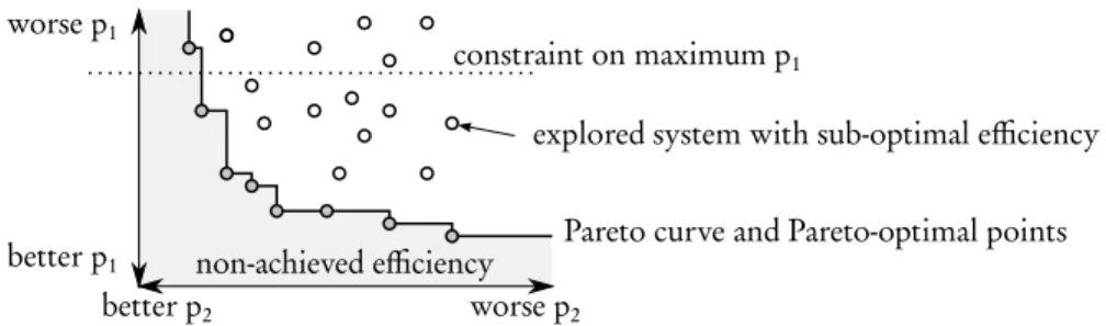
The holistic optimisation of a system in its different aspects is called Design Space Exploration (DSE) [31]. Exploring the design space consists in creating a Pareto chart such as the one in Figure 1 and choosing solutions on the Pareto front, i.e. solutions that represent the best alternative in at least one dimension and respect constraints in the other dimensions. As an example, p1on Figure 1 can be energy
consumption and p2can be response time. Figure 1 illustrates in 2 dimensions a
problem that, in general, has many more dimensions. In order to make system-level design efficient, separation of concerns is desirable [16]. Separation of concerns refers to forcing decisions on different design concerns to be (nearly) independent. The separation of concerns between application and architecture design makes it possible to generate many points for the Pareto by varying separately application and architecture parameters and observing their effects on system efficiency.
better p1
better p2
worse p1
worse p2
constraint on maximum p1
Pareto curve and Pareto-optimal points explored system with sub-optimal efficiency non-achieved efficiency
Fig. 1 The problem of Design Space Exploration (DSE) illustrated on a 2-D Pareto chart with efficiency metrics p1and p2.
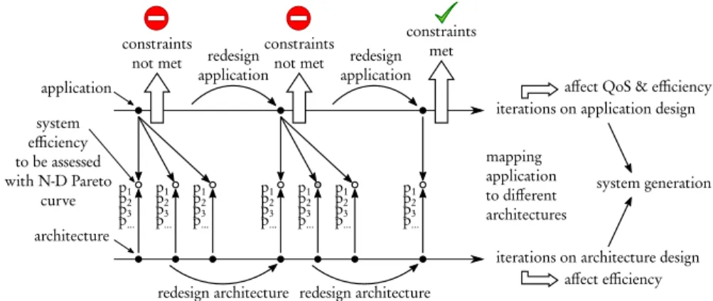
For example, the designer can build an application, test its efficiency on different platform architectures and, if constraints are not met by any point on the Pareto, iterate the process until reaching a satisfactory efficiency. This process is illustrated on Figure 2 and leads to Pareto points in Figure 1. Taking the hypothesis that a unique contraint is set on the maximum mp1of property p1, the first six generated
systems in Figure 2 led to p1> mp1 (corresponding to points over the dotted line
in Figure 1) and different values of p2, p3, etc. The seventh generated system has
p1≤ mp1and thus respects the constraint. Further system generations can be
per-formed to optimize p2, p3, etc. and generate the points under the dotted line in
Figure 1. Such a design effort is feasible only if application and architecture can be played with efficiently. On the application side, this is possible using Models of Computation (MoCs) that represent the high-level aspects (e.g. parallelism, ex-changed data, triggering events...) of an application while hiding its detailed imple-mentation. Equivalently on the architectural side, Models of Architecture (MoAs) can be used to extract the fundamental elements affecting efficiency while ignor-ing the details of circuitry. This chapter aims at reviewignor-ing languages and tools for modeling architectures and precisely defining the scope and capabilities of MoAs.
The chapter is organised as follows. The context of MoAs is first explained in Section 2. Then, definitions of an MoA and a quasi-MoA are argued in Section 3. Sections 4 and 5 give examples of state of the art quasi-MoAs. Finally, Section 6 concludes this chapter.
iterations on application design
iterations on architecture design system generation redesign
application applicationredesign
constraints
not met constraintsnot met
constraints met mapping application to different architectures system efficiency to be assessed with N-D Pareto curve
redesign architecture redesign architecture
affect QoS & efficiency
affect efficiency application architecture p1 p2 p3 p... p1 p2 p3 p... p1 p2 p3 p... p1 p2 p3 p... p1 p2 p3 p... p1 p2 p3 p... p1 p2 p3 p...
Fig. 2 Example of an iterative design process where application is refined and, for each refinement step, tested with a set of architectures to generate new points for the Pareto chart.
2 The Context of Models of Architecture
2.1 Models of Architecture in the Y-Chart Approach
The main motivation for developing Models of Architecture is for them to formalize the specification of an architecture in a chart approach of system design. The Y-chart approach, introduced in [18] and detailed in [2], consists in separating in two independent models the application-related and architecture-related concerns of a system’s design.
This concept is refined in Figure 3 where a set of applications is mapped to a set of architectures to obtain a set of efficiency metrics. In Figure 3, the application model is required to conform to a specified MoC and the architecture model is re-quired to conform to a specified MoA. This approach aims at separating What is implemented from How it is implemented. In this context, the application is qual-ified by a Quality of Service (QoS) and the architecture, offering resources to this application, is characterized by a given efficiency when supporting the application. For the discussion not to remain abstract, next section illustrates the problem on an example.
Model of Architecture Model of
Computation Application
Mapper and Simulator
conform to
What
How
conform to Architecture p1 efficiency metrics p2 p3 ... redesign ifnon-satisfactory redesign if non-satisfactory
Fig. 3 MoC and MoA in the Y-chart [18].
2.2 Illustrating Iterative Design Process and Y-Chart on an
Example System
QoS and efficiency metrics are multi-dimensional and can take many forms. For a signal processing application, QoS may be the Signal-to-Noise Ratio (SNR) or the Bit Error Rate (BER) of a transmission system, the compression rate of an encoding application, the detection precision of a radar, etc. In terms of architectural deci-sions, the obtained set of efficiency metrics is composed of some of the following Non-Functional Properties (NFPs):
• over time:
– latency (also called response time) corresponds to the time duration between the arrival time of data to process and the production time of processed data, – throughput is the amount of processed data per time iterval,
– jitter is the difference between maximal and minimal latency over time, • over energy consumption:
– energy corresponds to the energy consumed to process an amount of data, – peak power is the maximal instantaneous power required on alimentation to
process data,
– temperature is the effect of dissipated heat from processing, • over memory:
– Random Access Memory (RAM) requirements corresponds to the amount of necessary read-write memory to support processing,
– Read-Only Memory (ROM) requirements is the amount of necessary read-only memory to support processing,
• over security:
– electromagnetic interference corresponds to the amount of non-desired emit-ted radiations,
• over space:
– area is the total surface of semiconductor required for a given processing, – volume corresponds to the total volume of the built system.
– weight corresponds to the total weight of the built system.
• and cost corresponds to the monetary cost of building one system unit under the assumption of a number of produced units.
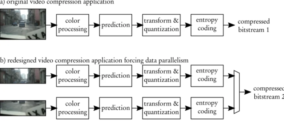
The high complexity of automating system design with a Y-chart approach comes from the extensive freedom (and imagination) of engineers in redesigning both ap-plication and architecture to fit the efficiency metrics, among this list, falling into their applicative constraints. Figure 4 is an illustrating example of this freedom on the application side. Let us consider a video compression system, borrowed from Chapter [6], to be ported on a platform. As shown in Figure 4 a), the application initially has only pipeline parallelism. Assuming that all four tasks are equivallent in complexity and that they receive and send at once a full image as a message, pipelining can be used to map the application to a multicore processor with 4 cores, with the objective to rise throughput (in frames per second) when compared to a monocore execution. However, latency will not be reduced because data will have to traverse all tasks before being output. In Figure 4 b), the image has been split into two halves and each half is processed independently. The application QoS in this second case will be lower, as the redundancy between image halves is not used for compression. The compression rate or image quality will thus be degraded. How-ever, by accepting QoS reduction, the designer has created data parallelism that offers new opportunities for latency reduction, as processing an image half will be faster than processing a whole image.
color
processing prediction transform &quantization entropycoding
color
processing prediction transform &quantization entropycoding color
processing prediction transform &quantization entropycoding
compressed bitstream 1
compressed bitstream 2 a) original video compression application
b) redesigned video compression application forcing data parallelism
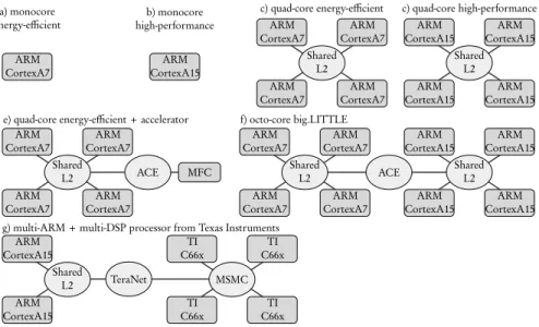
In terms of architecture, and depending on money and design time resources, the designer may choose to run some tasks in hardware and some in software over processors. He can also choose between different hardware interconnects to connect these architecture components. For illustrative purpose, Figure 5 shows different configurations of processors that could run the applications of Figure 4. rounded rectangles represent Processing Elements (PEs) performing computation while ovals represent Communication Nodes (CNs) performing inter-PE com-munication. Different combinations of processors are displayed, leveraging on high-performance out-of-order ARM Cortex-A15 cores, on high-efficiency in-order ARM Cortex-A7 cores, on the Multi-Format Codec (MFC) hardware accelerator for video encoding and decoding, or on Texas Instruments C66x Digital Signal Process-ing cores. Figure 5 g) corresponds to a 66AK2L06 Multicore DSP+ARM KeyStone II processor from Texas Instruments where ARM Cortex-A15 cores are combined with C66x cores connected with a Multicore Shared Memory Controller (MSMC) [36]. In these examples, all PEs of a given type communicate via shared mem-ory with either hardware cache coherency (Shared L2) or software cache coherency (MSMC), and with each other using either the Texas Instruments TeraNet switch fab-ric or the ARM AXI Coherency Extensions (ACE) with hardware cache coherency [35].
ARM
CortexA7 CortexA7ARM
ARM
CortexA7 CortexA7ARM
Shared L2
ARM
CortexA15 CortexA15ARM
ARM
CortexA15 CortexA15ARM
Shared L2 ACE
ARM
CortexA7 CortexA7ARM
ARM
CortexA7 CortexA7ARM
Shared L2 ACE MFC ARM CortexA7 a) monocore energy-efficient ARM CortexA15 b) monocore high-performance ARM
CortexA7 CortexA7ARM
ARM
CortexA7 CortexA7ARM
Shared L2 c) quad-core energy-efficient
e) quad-core energy-efficient + accelerator f) octo-core big.LITTLE
ARM
CortexA15 CortexA15ARM
ARM
CortexA15 CortexA15ARM
Shared L2 c) quad-core high-performance ARM CortexA15 ARM CortexA15 Shared L2 TI C66x C66x TI TI C66x C66xTI MSMC TeraNet
g) multi-ARM + multi-DSP processor from Texas Instruments
Fig. 5 Illustrating designer’s freedom on the architecture side with some current ARM-based and Digital Signal Processor-based multi-core architectures.
Each architecture configuration and each mapping and scheduling of the appli-cation onto the architecture leads to different efficiencies in all the previously listed NFPs. Considering only one mapping per application-architecture couple, models from Figures 4 and 5 already define 2 × 7 = 14 systems. Adding mapping choices
of tasks to PEs, and considering that they all can execute any of the tasks and ig-noring the order of task executions, the number of possible system efficiency points in the Pareto Chart is already roughly 19.000.000. This example shows how, by modeling application and architecture independently, a large number of potential systems is generated which makes automated multi-dimensional DSE necessary to fully explore the design space.
2.3 On the separation between application and architecture
concerns
Separation between application and architectural concerns should not be confused with software (SW)/hardware (HW) separation of concerns. The software/hardware separation of concerns is often put forward in the term HW/SW co-design. Soft-ware and its languages are not necessarily architecture-agnostic representations of an application and may integrate architecture-oriented features if the performance is at stake. This is shown for instance by the differences existing between the C++ and CUDA languages. While C++ builds an imperative, object-oriented code for a processor with a rather centralized instruction decoding and execution, CUDA is tailored to GPGPUs with a large set of cores. As a rule of thumb, software qualifies what may be reconfigured in a system while hardware qualifies the static part of the system.
The separation between application and architecture is very different in the sense that the application may be transformed into software processes and threads, as well as into hardware Intellectual Property cores (IPs). Software and Hardware applica-tion parts may collaborate for a common applicative goal. In the context of DSP, this goal is to transform, record, detect or synthetize a signal with a given QoS. MoCs follow the objective of making an application model agnostic of the architectural choices and of the HW/SW separation. The architecture concern relates to the set of hardware and software support features that are not specific to the DSP process, but create the resources handling the application.
On the application side, many MoCs have been designed to represent the behav-ior of a system. The Ptolemy II project [7] has a considerable influence in promoting MoCs with precise semantics. Different families of MoCs exist such as finite state machines, process networks, Petri nets, synchronous MoCs and functional MoCs. This chapter defines MoAs as the architectural counterparts of MoCs and presents a state-of-the-art on architecture modeling for DSP systems.
2.4 Scope of this chapter
In this chapter, we focus on architecture modeling for the performance estimation of a DSP application over a complex distributed execution platform. We keep
func-tional testing of a system out of the scope of the chapter and rather discuss the early evaluation of system non-functional properties. As a consequence, virtual platforms such as QEMU [3], gem5 [4] or Open Virtual Platforms simulator (OVPsim), that have been created as functional emulators to validate software when silicon is not available, will not be discussed. MoAs work at a higher level of abstraction where functional simulation is not central.
The considered systems being dedicated to digital signal processing, the study concentrates on signal-dominated systems where control is limited and provided together with data. Such systems are called transformational, as opposed to reactive systems that can, at any time, react to non-data-carrying events by executing tasks.
Finally, the focus is put on system-level models and design rather than on de-tailed hardware design, already addressed by large sets of existing literature. Next section introduces the concept of an MoA, as well as an MoA example named Linear System-Level Architecture Model (LSLA).
3 The Model of Architecture Concept
The concept of MoA is evoked in 2002 in [19] where it is defined as “a formal rep-resentation of the operational semantics of networks of functional blocks describing architectures”. This definition is broad, and allows the concepts of MoC and MoA to overlap. As an example, a Synchronous Dataflow (SDF) graph [24] [14] repre-senting a system fully specialized to an application may be considered as a MoC, because it formalizes the application. It may also be considered as an MoA because it fully complies with the definition from [19]. The Definition 4 of this chapter, adapted from [30], is a new definition of an MoA that does not overlap with the concept of MoC. The LSLA model is then presented to clarify the concept by an example.
3.1 Definition of an MoA
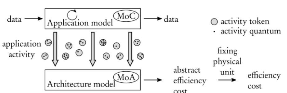
Prior to defining MoA, the notion of application activity is introduced that en-sures the separation of MoC and MoA. Figure 6 illustrates how application activity provides intermediation between application and architecture. Application activity models the computational load handled by the architecture when executing the ap-plication.
Definition 1. Application activityA corresponds to the amount of processing and communication necessary for accomplishing the requirements of the considered ap-plication during the considered time slot. Apap-plication activity is composed of pro-cessing and communication tokens, themselves composed of quanta.
Application model MoC
Architecture modelMoA application activity abstract efficiency cost activity token activity quantum data data efficiency cost fixing physical unit
Fig. 6 Application activity as an intermediate model between application and architecture.
Definition 2. A quantum q is the smallest unit of application activity. There are two types of quanta: processing quantum qPand communication quantum qC.
Two distinct processing quanta are equivalent, thus represent the same amount of activity. Processing and communication quanta do not share the same unit of measurement. As an example, in a system with a unique clock and byte-addressable memory, 1 cycle of processing can be chosen as the processing quantum and 1 byte as the communication quantum.
Definition 3. A token τ ∈ TP∪ TCis a non-divisible unit of application activity,
com-posed of a number of quanta. The function size : TP∪ TC → N associates to each
token the number of quanta composing the token. There are two types of tokens: processing tokens τP∈ TPand communication tokens τC∈ TC.
The activityA of an application is composed of the set:
A = {TP, TC} (1)
where TP= {τP1, τP2, τP3...} is the set of processing tokens composing the application
processing and TC = {τC1, τC2, τC3...} is the set of communication tokens composing
the application communication.
An example of a processing token is a run-to-completion task with always identi-cal computation. All tokens representing the execution of this task enclose the same number N of processing quanta (e.g. N cycles). An example of a communication token is a message in a message-passing system. The token is then composed of M communication quanta (e.g. M Bytes). Using the two levels of granularity of a token and a quantum, an MoA can reflect the cost of managing a quantum, and the additional cost of managing a token composed of several quanta.
Definition 4. A Model of Architecture (MoA) is an abstract efficiency model of a system architecture that provides a unique, reproducible cost computa-tion, unequivocally assessing an architecture efficiency cost when supporting the activity of an application described with a specified MoC.
This definition makes three aspects fundamental for an MoA:
• reproducibility: using twice the same MoC and activity computation with a given MoA, system simulation should return the exact same efficiency cost,
• application independence: the MoC alone carries application information and the MoA should not comprise application-related information such as the exchanged data formats, the task representations, the input data or the considered time slot for application observation. Application activity is an intermediate model be-tween a MoC and an MoA that prevents both models to intertwine. An applica-tion activitymodel reflects the computational load to be handled by architecture and should be versatile enough to support a large set of MoCs and MoAs, as demonstrated in [30].
• abstraction: a system efficiency cost, as returned by an MoA, is not bound to a physical unit. The physical unit is associated to an efficiency cost outside the scope of the MoA. This is necessary not to redefine the same model again and again for energy, area, weight, etc.
Definition 4 does not compel an MoA to match the internal structure of the hard-ware architecture, as long as the generated cost is of interest. An MoA for energy modeling can for instance be a set of algebraic equations relating application activ-ity to the energy consumption of a platform. To keep a reasonably large scope, this chapter concentrates on graphical MoAs defined hereafter:
Definition 5. A graphical MoA is an MoA that represents an architecture with a graph Λ = hM, L,t, pi where M is a set of “black-box” components and L⊆ M × M is a set of links between these components.
The graph Λ is associated with two functions t and p. The type function t: M × L 7→ T associates a type t ∈ T to each component and to each link. The type dedicates a component for a given service. The properties function p : M×L ×Λ 7→P(P), where P represents powerset, gives a set of properties pi∈
Pto each component, link, and to the graph Λ itself. Properties are features that relate application activity to implementation efficiency.
When the concept of MoA is evoked throughout this chapter, a graphical MoA is supposed, respecting Definition 5. When a model of a system architecture is evoked that only partially compels with this definition, the term quasi-MoA is used, equiv-alent to quasi-moa in [30] and defined hereafter:
Definition 6. A quasi-MoA is a model respecting some of the aspects of Definition 4 of an MoA but violating at least one of the three fundamental aspects of an MoA, i.e. reproducibility, application independence, and abstraction.
All state-of-the-art languages and models presented in Sections 4 and 5 define quasi-MoAs. As an example of a graphical quasi-MoAs, the graphical representa-tion used in Figure 5 shows graphs Λ = hM, Li with two types of components (PE
and CN), and one type of undirected link. However, no information is given on how to compute a cost when associating this representation with an application repre-sentation. As a consequence, reproducibility is violated. Next section illustrates the concept of MoA through the LSLA example.
3.2 Example of an MoA: the Linear System-Level Architecture
Model (LSLA)
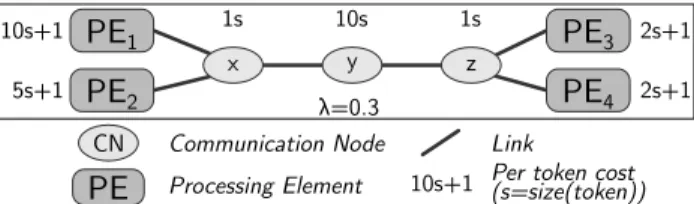
The LSLA model computes an additive reproducible cost from a minimalistic rep-resentation of an architecture [30]. As a consequence, LSLA fully complies with Definition 5 of a graphical MoA. The LSLA composing elements are illustrated in Figure 7. An LSLA model specifies two types of components: Processing Elements and Communication Nodes, and one type of link. LSLA is categorized as linear because the computed cost is a linear combination of the costs of its components.
Link
PE
Processing ElementCN Communication Node
10s+1 Per token cost(s=size(token)) z
PE
2 1s x y 10s 1sPE
1 10s+1 5s+1PE
4PE
3 2s+1 2s+1 λ=0.3Fig. 7 LSLA MoA semantics elements.
Definition 7. The Linear System-Level Architecture Model (LSLA) is a Model of Architecture (MoA) that consists of an undirected graph Λ = (P,C, L, cost, λ ) where:
• P is a set of Processing Elements (PEs). A PE is an abstract processing facility with no assumption on internal parallelism, Instruction Set Architecture (ISA), or internal memory. A processing token τP from application activity must be
mapped to a PE p ∈ P to be executed.
• C is the set of architecture Communication Nodes (CNs). A communication to-ken τCmust be mapped to a CN c ∈ C to be executed.
• L = {(ni, nj)|ni∈ C, nj∈ C ∪ P} is a set of undirected links connecting either two
CNs or one CN and one PE. A link models the capacity of a CN to communicate tokens to/from a PE or to/from another CN.
• cost is a property function associating a cost to different elements in the model. The cost unit is specific to the non-functional property being modeled. It may be in mJ for studying energy or in mm2for studying area. Formally, the generic unit is denoted ν.
On the example displayed in Figure 7, PE1−4 represent Processing Elements
(PEs) while x, y and z are Communication Nodes (CNs). As an MoA, LSLA provides reproducible cost computation when the activityA of an application is mappedonto the architecture. The cost related to the management of a token τ by a PE or a CN n is defined by:
cost: TP∪ TC× P ∪C → R τ , n 7→ αn.size(τ) + βn,
αn∈ R, βn∈ R
(2)
where αn is the fixed cost of a quantum when executed on n and βn is the fixed
overhead of a token when executed on n. For example, in an energy modeling use case, αnand βnare respectively expressed in energy/quantum and energy/token,
as the cost unit ν represents energy. A token communicated between two PEs con-nected with a chain of CNs Γ = {x, y, z...} is reproduced card(Γ ) times and each occurrence of the token is mapped to 1 element of Γ . This procedure is illustrated in Figure 8. In figures representing LSLA architectures, the size of a token size(τ) is abbreviated into s and the affine equations near CNs and PEs (e.g. 10s + 1) represent the cost computation related to Equation 2 with αn= 10 and βn= 1.
A token not communicated between two PEs, i.e. internal to one PE, does not cause any cost. The cost of the execution of application activity A on an LSLA graph Λ is defined as:
cost(A ,Λ) = ∑τ ∈T
Pcost(τ, map(τ))+
λ ∑τ ∈TCcost(τ, map(τ))
(3) where map : TP∪ TC→ P ∪C is a surjective function returning the mapping of each
token onto one of the architecture elements.
• λ ∈ R is a Lagrangian coefficient setting the Computation to Communication Cost Ratio (CCCR), i.e. the cost of a single communication quantum relative to the cost of a single processing quantum.
Similarly to the SDF MoC [24], the LSLA MoA does not specify relations to the outside world. There is no specific PEs type for communicating with non-modeled parts of the system. This is in contrast with Architecture Analysis and Design Lan-guage (AADL) processors and devices that separate I/O components from processing components (Section 4.1). The Definition 1 of activity is sufficient to support LSLA and other types of additive MoAs. Different forms of activities are likely to be necessary to define future MoAs. Activity Definition 1 is generic to several families of MoCs, as demonstrated in [30].
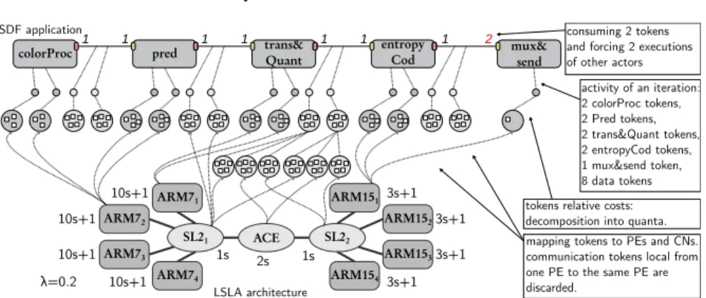
Figure 8 illustrates cost computation for a mapping of the video compression ap-plication shown in Figure 4 b), described with the SDF MoC onto the big.LITTLE architecture of Figure 5 f), described with LSLA. The number of tokens, quanta and the cost parameters are not representative of a real execution but set for illustra-tive purpose. The natural scope for the cost computation of a couple (SDF, LSLA), provided that the SDF graph is consistent, is one SDF graph iteration [30].
LSLA architecture activity of an iteration: 2 colorProc tokens, 2 Pred tokens, 2 trans&Quant tokens, 2 entropyCod tokens, 1 mux&send token, 8 data tokens SDF application
tokens relative costs: decomposition into quanta. mapping tokens to PEs and CNs. communication tokens local from one PE to the same PE are discarded. λ=0.2 10s+1 10s+1 1s 2s 3s+1 3s+1 pred
colorProc 1 1 1 1 trans&Quant 1 1 entropyCod 1 2 mux&send
ARM72 ARM73 1s ARM71 ARM74 ARM152 ARM153 ARM151 ARM154 10s+1 10s+1 3s+1 3s+1 SL21 ACE SL22 consuming 2 tokens and forcing 2 executions of other actors
Fig. 8 Computing cost of executing an SDF graph on an LSLA architecture. The cost for 1 iteration is (looking first at processing tokens then at communication tokens from left to right) 31 + 31 + 41 + 41 + 41 + 41 + 13 + 13 + 4 + 0.2 × (5 + 5 + 5 + 10 + 5 + 5 + 10 + 5) = 266 ν (Equation 3).
The SDF application graph has 5 actors colorProc, pred, trans&Quant, entropy-Cod, and mux&Send and the 4 first actors will execute twice to produce the 2 image halves required by mux&Send. The LSLA architecture model has 8 PEs ARM jk
with j ∈ {7, 15} and k ∈ {1, 2, 3, 4}, and 3 CNs SL21, ACE and SL22. Each actor
ex-ecution during the studied graph iteration is transformed into one processing token. Each dataflow token transmitted during one iteration is transformed into one com-munication token. A token is embedding several quanta (white squares), allowing a designer to describe heterogeneous tokens to represent executions and messages of different weight.
In Figure 8, each execution of actors colorProc is associated with a cost of 3 quanta and each execution of other actors is associated to a cost of 4 quanta except mux&Send requiring 1 quantum. Communication tokens (representing one half im-age transfer) are given 5 quanta each. These costs are arbitrary here but should represent the relative computational load of the task/communication.
Each processing token is mapped to one PE. Communication tokens are “routed” to the CNs connecting their producer and consumer PEs. For instance, the fifth and sixth communication tokens in Figure 8 are generating 3 tokens each mapped to SL21, ACE and SL22because the data is carried from ARM71to ARM151. It is the
responsibility of the mapping process to verify that a link l ∈ L exists between the elements that constitute a communication route. The resulting cost, computed from Equations 2 and 3, is 266ν. This cost is reproducible and abstract, making LSLA an MoA.
LSLA is one example of an architecture model but many such models exist in literature. Next sections study different languages and models from literature and explain the quasi-MoAs they define.
4 Architecture Design Languages and their Architecture Models
This section studies the architecture models provided by three standard Architecture Design Languages (ADLs) targeting architecture modeling at system-level: AADL, MCA SHIM, and UML MARTE.
While AADL adopts an abstraction/refinement approach where components are first roughly modeled, then refined to lower levels of abstraction, UML MARTE is closer to a Y-Chart approach where the application and the architecture are kept separated and application is mapped to architecture.
For its part, MCA SHIM describes an architecture with “black box” processors and communications and puts focus on inter-PE communication simulation. All these languages have in common the implicit definition of a quasi-MoA (Defini-tion 6). Indeed, while they define parts of graphical MoAs, none of them respect the 3 rules of MoA Definition 4.
4.1 The AADL Quasi-MoA
Architecture Analysis and Design Language (AADL) [9] is a standard language released by SAE International, an organization issuing standards for the aerospace and automotive sectors. The AADL standard is referenced as AS5506 [33] and the last released version is 2.2. Some of the most active tools supporting AADL are Ocarina1[21] and OSATE2[9].
4.1.1 The Features of the AADL Quasi-MoA
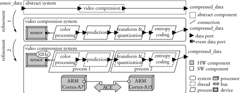
AADL provides semantics to describe a software application, a hardware platform, and their combination to form a system. AADL can be represented graphically, se-rialized in XML or described in a textual language [10]. The term architecture in AADL is used in its broadest sense, i.e. a whole made up of clearly separated el-ements. A design is constructed by successive refinements, filling “black boxes” within the AADL context. Figure 9 shows two refinement steps for a video com-pression system in a camera. Blocks of processing are split based on the application decomposition of Figure 4 a). First, the system is abstracted with external data enter-ing a video compression abstract component. Then, 4 software processes are defined for the processing. Finally, processes are transformed into 4 threads, mapped onto 2 processes. The platform is defined with 2 cores and a bus and ap-plication threads are allocated onto platform components. The allocation of threads to processors is not displayed. Sensor data is assigned a rate of 30 Hz,
correspond-1https://github.com/OpenAADL/ocarina 2https://github.com/osate
ing to 30 frames per second. Next sections detail the semantics of the displayed components.
abstract system
video compression video compression system
sensor_data
compressed_data
sensor processingcolor prediction transform &quantization entropycoding compressed_data video compression system
sensor processingcolor prediction transform &quantization entropycoding
compressed_data ACE process 1 process 2 30Hz re finement 1 re finement 2 ARM
Cortex-A7 Cortex-A15ARM
HW component SW component thread process processor bus device abstract component data port event data port
system connection
Fig. 9 The AADL successive refinement system design approach.
Software, hardware and systems are described in AADL by a composition of components. In this chapter, we focus on the hardware platform modeling ca-pabilities of AADL, composing an implicit graphical quasi-MoA. Partly respecting Definition 5, AADL represents platform with a graph Λ = hM, L,t, pi where M is a set of components, L is a set of links, t associates a type to each component and link and p gives a set of properties to each component and link. As displayed in Figure 10, AADL defines 6 types of platform components with specific graphical representations. The AADL component type set is such that t(c ∈ M) ∈ {system, processor, device, bus, memory, abstract}. There is one type of link t(l ∈ L) ∈ {connection}. A connection can be set between any two com-ponents among software, hardware or system. Contrary to the Y-chart approach, AADL does not separate application from architecture but makes them coexist in a single model.
device bus
processor memory
system abstract
Fig. 10 The basic components for describing a hardware architecture in AADL.
AADL is an extensible language but defines some standard component prop-erties. These properties participate to the definition of the quasi-MoA determined by the language and make an AADL model portable to several tools. The AADL standard set of properties targets only the time behavior of components and differs for each kind of component. AADL tools are intended to compute NFP costs such as the total minimum and maximum execution latency of an application, as well as the jitter. An AADL representation can also be used to extract an estimated bus bandwidth or a subsystem latency [20].
Processors are sequential execution facilities that must support thread schedul-ing, with a protocol fixed as a property. AADL platform components are not merely hardware models but rather model the combination of hardware and low-level soft-ware that provides services to the application. In that sense, the architecture model they compose is conform to MoA Definition 4. However, what is mapped on the platform is software rather than an application. As a consequence, the separation of concerns between application and architecture is not supported (Section 2.3). For instance, converting the service offered by a software thread to a hardware IP neces-sitates to deeply redesign the model. A processor can specify a Clock Period, a Thread Swap Execution Time and an Assign Time, quantifying the time to access memory on the processor. Time properties of a processor can thus be precisely set.
A bus can specify a fixed Transmission Time interval representing best- and worst-case times for transmitting data, as well as a PerByte Transmission Time interval representing throughput. The time model for a message is thus an affine model w.r.t. message size. Three models for transfer cost computation are displayed in Figure 11: linear, affine, and stair. Most models discussed in the next sections use one of these 3 models. The interpretation of AADL time properties is precisely defined in [9] Appendix A, making AADL time computation reproducible.
message size N comm unica tion cos t ζ off se t start step_width step_height stair message cost from equation (1) 800 700 600 500 400 300 200 100 00 100 200 300 400 500600 700 800 900 1000 affine message cost
linear message cost
Fig. 11 Examples of different data transfer cost computation functions (in arbitrary units): a linear function (with 1 parameter), an affine function (with 2 parameters) and a step function (with 4 parameters).
A memory can be associated to a Read Time, a Write Time, a Word Count and a Word Size to characterize its occupancy rate. A device can be associated to a Period, and a Compute Execution Time to study sensors’ and actuators’ latency and throughput. Platform components are defined to support a software application. The next section studies application and platform interactions in AADL.
4.1.2 Combining Application and Architecture in AADL
AADL aims at analyzing the time performance of a system’s architecture, man-ually exploring the mapping (called binding in AADL) of software onto hard-ware elements. AADL quasi-MoA is influenced by the supported softhard-ware model. AADL is adapted to the currently dominating software representation of Operating Systems (OS), i.e. the process and thread representation [9]. An application is de-composed into process and thread components, that are purely software concepts. A process defines an address space and a thread comes with scheduling policies and shares the address space of its owner process. A process is not executable by itself; it must contain a least one thread to execute. AADL Threads are sequential, preemptive entities [9] and requires scheduling by a processor. Threads may specify a Dispatch Protocol or a Period property to model a periodic behavior or an event-triggered callback or routine.
A values or interval of Compute Execution Time can be associated to a thread. However, in real world, execution time for a thread firing depends on both the code to execute and the platform speed. Compute Execution Time is not related to the binding of the thread to a processor but a Scaling Factor property can be set on the processor to specify its relative speed with regards to a reference processor for which thread timings have been set. This property is precise when all threads on a processor undergo the same Scaling Factor, but this is not the case in general. For instance, if a thread compiled for the ARMv7 instruction set is first executed on an ARM Cortex-A7 and then on an ARM Cortex-A15 processor, the observed speedup depends much on the executed task. Speedups between 1.3× and 4.9× are reported in this context in [30].
AADL provides constructs for data message passing through port features and data memory-mapped communication through require data access features. These communications are bound to busses to evaluate their timings.
A flow is neither a completely software nor a completely hardware construct. It specifies an end-to-end flow of data between sensors and actuators for steady state and transient timing analysis. A flow has timing properties such as Expected Latency and Expected Throughput that can be verified through simulation.
4.1.3 Conclusions on the AADL Quasi-MoA
AADL specifies a graphical quasi-MoA, as it does define a graph of platform com-ponents. AADL violates the abstraction rule because cost properties are explicitly time and memory. It respects the reproducibility rule because details of timing sim-ulations are precisely defined in the documentation. Finally, it violates the applica-tion independencerule because AADL does not conform to the Y-chart approach and does not separate application and architecture concerns.
AADL is a formalization of current best industrial practices in embedded system design. It provides formalization and tools to progressively refine a system from an abstract view to a software and hardware precise composition. AADL targets
all kinds of systems, including transformational DSP systems managing data flows but also reactive system, reacting to sporadic events. The thread MoC adopted by AADL is extremely versatile to reactive and transformational systems but has shown its limits for building deterministic systems [23] [37]. By contrast, the quasi-MoAs presented in Section 5 are mostly dedicated to transformational systems. They are thus all used in conjunction with process network MoCs that help building reli-able DSP systems. The next section studies another state-of-the-art language: MCA SHIM.
4.2 The MCA SHIM Quasi-MoA
The Software/Hardware Interface for Multicore/Manycore (SHIM) [12] is a hard-ware description language that aims at providing platform information to multicore software tools, e.g. compilers or runtime systems. SHIM is a standard developed by the Multicore Association (MCA). The most recent released version of SHIM is 1.0 (2015) [27]. SHIM is a more focused language than AADL, modeling the platform properties that influence software performance on multicore processors.
SHIM components provide timing estimates of a multicore software. Contrary to AADL that mostly models hard real-time systems, SHIM primarily targets best-effort multicore processing. Timing properties are expressed in clock cycles, sug-gesting a fully synchronous system. SHIM is built as a set of UML classes and the considered NFPs in SHIM are time and memory. Timing performances in SHIM are set by a shim::Performance class that characterizes three types of software ac-tivity: instruction executions for instructions expressed in the LLVM instruction set, memory accesses, and inter-core communications. LLVM [22] is used as a portable assembly code, capable of decomposing a software task into instructions that are portable to different ISAs.
SHIM does not propose a chart representation of its components. However, SHIM defines a quasi-MoA partially respecting Definition 5. A shim::System-Configurationobject corresponds to a graph Λ = hM, L,t, pi where M is the set of components, L is the set of links, t associates a type to each component and link and p gives a set of properties to each component and link. A SHIM archi-tecture description is decomposed into three main sets of elements: Components, Address Spacesand Communications. We group and rename the compo-nents (referred to as “objects” in the standard) to makes them easier to compare to other approaches. SHIM defines 2 types of platform components. The component types t(c ∈ M) are chosen among:
• processor (shim::MasterComponent), representing a core executing soft-ware. It internally integrates a number of cache memories (shim::Cache) and is capable of specific data access types to memory (shim::AccessType). A processorcan also be used to represent a Direct Memory Access (DMA), • memory (shim::SlaveComponent) is bound to an address space
Links t(l ∈ L) are used to set performance costs. They are chosen among: • communication between two processors. It has 3 subtypes:
– fifo (shim::FIFOCommunication) referring to message passing with buffer-ing,
– sharedRegister (shim::SharedRegisterCommunication) referring to a semaphore-protected register,
– event (shim::EventCommunication for polling or shim::InterruptCommuni-cation for interrupts) referring to inter-core synchronization without data transfer.
• memoryAccess between a processor and a memory (modeled as a cou-ple shim::MasterSlaveBinding, shim::Accessor) sets timings to each type of data read/write accesses to the memory.
• sharedMemory between two processors (modeled as a triple shim::-SharedMemoryCommunication, shim::MasterSlaveBinding, and shim::Accessor) sets timing performance to exchanging data over a shared memory,
• InstructionExecution (modeled as a shim::Instruction) between a pro-cessor and itself sets performance on instruction execution.
Links are thus carrying all the performance properties in this model. Application activity on a link l is associated to a shim::Performance property, decomposed into latency and pitch. Latency corresponds to a duration in cycles while pitch is the inverse (in cycles) of the throughput (in cycles−1) at which a SHIM object can be managed. A latency of 4 and a pitch of 3 on a communication link, for instance, mean that the first data will take 4 cycles to pass through a link and then 1 data will be sent per 3 cycles. This choice of time representation is characteristic of the SHIM objective to model the average behavior of a system while AADL targets real-time systems. Instead of specifying time intervals [min..max] like AADL, SHIM defines triplets [min, mode, max] where mode is the statistical mode. As a consequence, a richer communication and execution time model can be set in SHIM. However, no information is given on how to use these performance properties present in the model. In the case of a communication over a shared memory for instance, the deci-sion on whether to use the performance of this link or to use the performance of the shared memory data accesses, also possible to model, is left to the SHIM supporting tool.
4.2.1 Conclusions on MCA SHIM Quasi-MoA
MCA SHIM specifies a graphical quasi-MoA, as it defines a graph of platform com-ponents. SHIM violates the abstraction rule because cost properties are limited to time. It also violates the reproducibility rule because details of timing simulations are left to the interpretation of the SHIM supporting tools. Finally, it violates the application independencerule because SHIM supports only software, decomposed into LLVM instructions.
The modeling choices of SHIM are tailored to the precise needs of multicore tooling interoperability. The two types of tools considered as targets for the SHIM standard are Real-Time Operating Systems (RTOSs) and auto-parallelizing compil-ers for multicore processors. The very different objectives of SHIM and AADL have led to different quasi-MoAs. The set of components is more limited in SHIM and communication with the outside world is not specified. The communication modes between processors are also more abstract and associated to more sophisticated tim-ing properties. The software activity in SHIM is concrete software, modeled as a set of instructions and data accesses while AADL does not go as low in terms of modeling granularity. To complement the study on a third language, the next section studies the different quasi-MoAs defined by the Unified Modeling Language (UML) Modeling And Analysis Of Real-Time Embedded Systems (MARTE) language.
4.3 The UML MARTE Quasi-MoAs
The UML Profile for Modeling And Analysis Of Real-Time Embedded Systems (MARTE) is standardized by the Object Management Group (OMG) group. The last version is 1.1 and was released in 2011 [28]. Among the ADLs presented in this chapter, UML MARTE is the most complex one. It defines hundreds of UML classes and has been shown to support most AADL constructs [8]. MARTE is de-signed to coordinate the work of different engineers within a team to build a com-plex real-time embedded system. Several persons, expert in UML MARTE, should be able to collaborate in building the system model, annotate and analyze it, and then build an execution platform from its model. Like AADL, UML MARTE is fo-cused on hard real-time application and architecture modeling. MARTE is divided into four packages, themselves divided into clauses. 3 of these clauses define 4 dif-ferent quasi-MoAs. These quasi-MoAs are named QMoAiMART E | i ∈ {1, 2, 3, 4} in this chapter and are located in the structure of UML MARTE clauses illustrated by the following list:
• The MARTE Foundations package includes:
– the Core Elements clause that gathers constructs for inheritance and composi-tion of abstract objects, as well as their invocacomposi-tion and communicacomposi-tion. – the Non-Functional Property (NFP) clause that describes ways to specify
non-functional constraints or values (Section 2.2), with a concrete type. – the Time clause, specific to the time NFP.
– the Generic Resource Modeling (GRM) clause that offers constructs to model, at a high level of abstraction, both software and hardware elements. It defines a generic component named Resource, with clocks and non-functional properties. Resource is the basic element of UML MARTE models of architecture and application. The quasi-MoA QMoA1MART Eis defined by GRM and based on Resources. It will be presented in Section 4.3.1.
– the Allocation Modeling clause that relates higher-level Resources to lower-level Resources. For instance, it is used to allocate Schedulable-Resources(e.g. threads) to ComputingResources (e.g. cores). • The MARTE Design Model package includes:
– the Generic Component Model (GCM) clause that defines structured compo-nents, connectors and interaction ports to connect core elements.
– the Software Resource Modeling (SRM) clause that details software resources. – the Hardware Resource Modeling (HRM) clause that details hardware
re-sources and defines QMoA2MART E and QMoA3MART E (Section 4.3.2).
– the High-Level Application Modeling (HLAM) clause that models real-time services in an OS.
• The MARTE Analysis Model package includes:
– the Generic Quantitative Analysis Modeling (GQAM) clause that specifies methods to observe system performance during a time interval. It defines QMoA4MART E.
– the Schedulability Analysis Modeling (UML MARTE) (SAM) clause that refers to thread and process schedulability analysis. It builds over GQAM and adds scheduling-related properties to QMoA4
MART E.
– the Performance Analysis Modeling (PAM) clause that performs probabilistic or deterministic time performance analysis. It also builds over GQAM. • MARTE Annexes include Repetitive Structure Modeling (RSM) to compactly
rep-resent component networks, and the Clock Constraint Specification Language (CCSL)to relate clocks.
The link between application time and platform time in UML MARTE is estab-lished through clock and event relationships expressed in the CCSL language [25]. Time may represent a physical time or a logical time (i.e. a continuous repetition of events). Clocks can have causal relations (an event of clock A causes an event of clock B) or a temporal relations with type precedence, coincidence, and exclu-sion. Such a precise representation of time makes UML MARTE capable of mod-eling both asynchronous and synchronous distributed systems [26]. UML MARTE is capable, for instance, of modeling any kind of processor with multiple cores and independent frequency scaling on each core.
The UML MARTE resource composition mechanisms give the designer more freedom than AADL by dividing his system into more than 2 layers. For instance, execution platform resources can be allocated to operating system resources, themselves allocated to application resources while AADL offers only a hardware/software separation. Multiple allocations to a single resource are either time multiplexed (timeScheduling) or distributed in space (spatialDistri-bution). Next sections explain the 4 quasi-MoAs defined by UML MARTE.
4.3.1 The UML MARTE Quasi-MoAs 1 and 4
The UML MARTE GRM clause specifies the QMoA1MART E quasi-MoA. It corre-sponds to a graph Λ = hM, L,t, pi where M is a set of Resources, L is a set of UML Connectors between these resources, t associates types to Resources and p gives sets of properties to Resources.
«Processing Resource» specializes
«Computing Resource» «Communication Media» «Device Resource»
«Storage Resource» «Synchronization Resource» «Timing Resource»
«Concurrency Resource»
Fig. 12 Elements of the quasi-MoA define in UML MARTE Generic Resource Modeling (GRM).
7 types of resources are defined in GRM. Some inconsistencies between re-source relations make the standard ambiguous on rere-source types. As an example, CommunicationMediaspecializes CommunicationResource on standard p.96 [28] while CommunicationMedia specializes ProcessingResource on standard p.99. SynchResource disappears after definition and is possibly equivalent to the later SwSynchronizationResource. Considering the most detailed descriptions as reference, types of resources (illustrated in Figure 12) are: • a Processing Resource, associated to an abstract speed Factor property
that can help the designer compare different Processing Resources. It has 3 subtypes: Computing Resource models a real or virtual PE storing and executing program code. It has no property. Device Resource commu-nicates with the system environment, equivalently to an AADL device. It also has no property. Communication Media can represent a bus or a higher-level protocol over an interconnect. It has several properties: a mode among sim-plex, half-dusim-plex, or full-duplex specifies whether the media is directed or not and the time multiplexing method for data. Communication Media trans-fers one data of elementSize bits per clock cycle. A packet time represents the time to transfer a set of elements. A block time represents the time before the media can transfer other packets. A data rate is also specified.
• a Timing Resource representing a clock or a timer, fixing a clock rate. • a Storage Resource representing memory, associated with a unit size and
number of units. Memory read and write occur in 1 clock cycle.
• a Concurrency Resource representing several concurrent flows of execu-tion. It is a generalization of SchedulableResources that model logical concurrency in threads and processes.
The communication time model of QMoA1MART E, set by the Communication Media, is the affine model illustrated in Figure 11. Precise time properties are set but the way to correctly compute a timing at system-level from the set of resource timings is not explicitly elucidated.
QMoA1
MART Ecan be used for more than just time modeling. ResourceUsage
occur, amounts of physical resources can be specified as “consumed”. A resource consumption amount can be associated to the following types of NFPs values: en-ergy in Joules, message size in bits, allocated memory in bytes, used memory in bytes (representing temporary allocation), and power peak in Watts.
The Generic Quantitative Analysis Modeling (GQAM) package defines another quasi-MoA (QMoA4
MART E) for performing the following set of analysis: counting
the repetitions of an event, determining the probability of an execution, determin-ing CPU requirements, determindetermin-ing execution latency, and determindetermin-ing throughput (time interval between two occurrences). New resources named GaExecHost (Ex-ecutionHost) and GaCommHost (CommunicationHost) are added to the ones of QMoA1MART E and specialize the ProcessingResource for time performance and schedulability analysis, as well as for the analysis of other NFPs. QMoA4MART E is thus close to QMoA1MART E in terms of resource semantics but additional proper-ties complement the quasi-MoA. In terms of MoAs, QMoA1MART Eand QMoA4MART E have the same properties and none of them clearly states how to use their properties.
4.3.2 The UML MARTE Quasi-MoAs 2 and 3
The UML MARTE Hardware Resource Modeling (HRM) defines two other, more complex quasi-MoAs than the previously presented ones: QMoA2
MART E (logical
view) and QMoA3MART E (physical view).
An introduction of the related software model is necessary before presenting hardware components because the HRM is very linked to the SRM software rep-resentation. In terms of software, the UML MARTE standard constantly refers to threads as the basic instance, modeled with a swSchedulableResource. The swSchedulableResources are thus considered to be managed by an RTOS and, like AADL, UML MARTE builds on industrial best practices of us-ing preemptive threads to model concurrent applications. In order to communicate, a swSchedulableResource references specifically defined software commu-nication and synchronization resources.
The HW Logical subclause of HRM refers to 5 subpackages: HW Computing, HW Communication, HW Storage, HW Device, and HW Timing. It com-poses a complex quasi-MoA referred to as QMoA2
MART E in this chapter. For brevity
and clarity, we will not enter the details of this quasi-MoA but give some informa-tion on its semantics.
The UML MARTE QMoA2MART Equasi-MoA is, like AADL, based on a HW/SW separation of concerns rather than on an application/architecture separation. In terms of hardware, UML MARTE tends to match very finely the real characteristics of the physical components. UML MARTE HRM is thus torn between the desire to match current hardware best practices and the necessity to abstract away system speci-ficities. A QMoA2MART E processing element for instance can be a processor, with an explicit Instruction Set Architecture (ISA), caches, and a Memory Management Unit (MMU), or it can be a Programmable Logic Device (PLD). In the description of a PLD, properties go down to the number of available Lookup Tables (LUTs) on the
PLD. However, modern PLDs such as Field-Programmable Gate Arrays (FPGAs) are far too heterogeneous to be characterized by a number of LUTs. Moreover, each FPGA has its own characteristics and in the space domain, for instance, FPGAs are not based on a RAM configuration memory, as fixed in the MARTE standard, but rather on a FLASH configuration memory. These details show the interest of abstracting an MoA in order to be resilient to the fast evolution of hardware archi-tectures.
HW Physicalcomposes the QMoA3MART Equasi-MoA and covers coarser-grain resources than QMoA2MART E, at the level of a printed circuit board. Properties of resources include shape, size, position, power consumption, heat dissipation, etc.
Interpreting the technological properties of HRM quasi-MoAs QMoA2MART E and QMoA3MART E is supposed to be done based on designer’s experience because the UML MARTE properties mirror the terms used for hardware design. This is how-ever not sufficient to ensure the reproducibility of a cost computation.
4.3.3 Conclusions on UML MARTE Quasi-MoAs
When considering as a whole the 4 UML MARTE quasi-MoAs, the standard does not specify how the hundreds of NFP standard resource parameters are to be used during simulation or verification. The use of these parameters is supposed to be transparent, as the defined resources and parameters match current best practices. However, best practices evolve over time and specifying precisely cost compu-tation mechanisms is the only way to ensure tool interoperability in the lon run. UML MARTE quasi-MoAs do not respect the abstraction rule of MoAs because, while cost properties target multiple NFPs, each is considered independently with-out capitalizing on similar behaviors of different NFPs. Finally, QMoA1MART E and QMoA4MART E respect the application independence rule, and even extend it to the construction of more than 2 layers, while QMoA2MART Eand QMoA3MART Erather pro-pose a HW/SW decomposition closer to AADL.
4.4 Conclusions on ADL Languages
AADL and UML MARTE are both complete languages for system-level design that offer rich constructs to model a system. MCA SHIM is a domain-specific language targeted to a more precise purpose. While the 3 languages strongly differ, they all specify quasi-MoAs with the objective of modeling the time behavior of a system, as well as other non-functional properties. None of these 3 languages fully respects the three rules of MoA’s Definition 4. In particular, none of them abstracts the studied NFPs to make generic the computation of a model’s cost from the cost of its con-stituents. Abstraction is however an important feature of MoAs to avoid redesigning redundant simulation mechanisms.
To complement this study on MoAs, the next section covers four formal quasi-MoAs from literature.
5 Formal Quasi-MoAs
In this Section, we put the focus on graphical quasi-MoAs that aim at providing system efficiency evaluations when combined with a model of a DSP application. The models and their contribution are presented chronologically.
5.1 The AAA Methodology Quasi-MoA
In 2003, an architecture model is defined for the Ad´equation Algorithm Architec-ture (AAA)Y-chart methodology, implemented in the SynDEx tool [13]. The AAA architecture model is tailored to the needs of an application model that splits pro-cessing into tasks called operations arranged in a Directed Acyclic Graph (DAG) representing data dependencies between them.
The AAA architecture model is a graphical quasi-MoA Λ = hM, L,t, pi, where M is a set of components, L is a set of undirected edges connecting these components, and t and p respectively give a type and a property to components. As illustrated in Figure 13, there are three types t ∈ T of components, each considered internally as a Finite State Machine (FSM) performing sequentially application management services : memory, sequencer, and bus/multiplexer/demultiplexer (B/M/D). For their part, edges only model the capacity of components to exchange data.
component
operator communicator RAM SAM RAMP RAMD RAMDP
memory B/M/D
sequencer
B/M/D with arb. B/M/D w/o arb. specializes
P D DP
arbiter
Fig. 13 Typology of the basic components in the AAA architecture model [13]. Leaf components are instantiable.
In this model, a memory is a Sequential Access Memory (SAM) or a Random Access Memory (RAM). A SAM models a First In, First Out data queue (FIFO) for message passing between components. A SAM can be point-to-point or multipoint and support or not broadcasting. A SAM with broadcasting only pops a data when all readers have read the data. A RAM may store only data (RAMD), only programs
(RAMP) or both (RAMDP). When several sequencers can write to a memory, it has
an implicit arbiter managing writing conflicts.
A sequencer is of type operator or communicator. An operator is a PE sequentially executing operations stored in a RAMPor RAMDP. An operation
reads and writes data from/to a RAMDor RAMDPconnected to the operator. A
communicatormodels a DMA with a single channel that executes communica-tions, i.e. operations that transfer data from a memory M1to a memory M2. For the
transfer to be possible, the communicator must be connected to M1and M2.
A B/M/D models a bus together with its multiplexer and demultiplexer that im-plement time division multiplexing of data. As a consequence, a B/M/D represents a sequential schedule of transfered data. A B/M/D may require an arbiter, solving write conflicts between multiple sources. In the AAA model, the arbiter has a max-imum bandwidth BPMax that is shared between writers and readers.
Figure 14 shows an example, inspired by [13], of a model conforming the AAA quasi-MoA. It models the 66AK2L06 processor [36] from Texas Instru-ments illustrated in Figure 5 g). Operators must delegate communication to communicatorsthat access their data memory. The architecture has hardware cache coherency on ARM side (L2CC for L2 Cache Control) and software cache coherency on c66x side (SL2C for Software L2 Coherency). The communication between ARML2 and MSMC memories is difficult to model with AAA FSM com-ponents because it is performed by a Network-on-Chip (NoC) with complex topol-ogy and a set of DMAs so it has been represented as a network of B/M/Ds and communicators in Figure 14. ARM Cortex-A15 TI c66x L2DP SL2C 1024KB L1PP 32KB MSMC DP 2048KB L2CC DMA DMA DMA TI c66x L2DP SL2C 1024KB TI c66x L2DP SL2C 1024KB TI c66x L2DP SL2C 1024KB TeraNetarbiter ARM Cortex-A15 32KBL1DD L2CC ARML2DP 1024KB TeraNetarbiter TeraNetarbiter ... ... DMA DMA DMA L1DD 32KB L1PP 32KB
Fig. 14 Example of an architecture description with the AAA quasi-MoA.
Properties p on components and edges define the quasi-MoA. An operator Ophas an associated function δOp setting a Worst Case Execution Time (WCET)
duration to each operation δOp(o) ∈ R≥0 where O is the set of all operations in
the application. This property results from the primary objective of the AAA ar-chitecture model being the computation of an application WCET. Each edge of the graph has a maximum bandwidth B in bits/s. The aim of the AAA quasi-MoA is to feed a multicore scheduling process where application operations are mapped to operatorsand data dependencies are mapped to routes between operators, made of communicators and busses. Each operator and communicator being an FSM, the execution of operations and communications on a given se-quencer is totally ordered. The application graph being a DAG, the critical path
of the application is computed and represents the latency of one execution, i.e. the time distance beween the beginning of the first operation and the end of the last operation. The computation of the latency from AAA application model and quasi-MoA in [13] is implicit. The behavior of the arbiter is not specified in the model so actual communication times are subject to interpretations, especially regarding the time quantum for the update of bandwidth utilization.
The AAA syntax-free quasi-MoA is mimicking the temporal behavior of a pro-cessing hardware in order to derive WCET information on a system. Many hard-ware features can be modeled, such as DMAs; shared memories and hardhard-ware FIFO queues. Each element in the model is sequential, making a coarse-grain model of an internally parallel component impossible. There is no cost abstraction but the sepa-ration between architecture model and application model is respected. The model is specific to dataflow application latency computation, with some extra features ded-icated to memory requirement computation. Some performance figures are subject to interpretation and latency computation for a couple application/architecture is not specified.
The AAA model contribution is to build a system-level architecture model that clearly separates architecture concerns from algorithm concerns. Next section dis-cusses a second quasi-MoA, named CHARMED.
5.2 The CHARMED Quasi-MoA
In 2004, the CHARMED co-synthesis framework [17] is proposed that aims at optimizing multiple system parameters represented in Pareto fronts. Such a multi-parameter optimization is essential for DSE activities, as detailed in [31].
In the CHARMED quasi-MoA Λ = hM, L,t, pi, M is a set of PEs, L is a set of Communication Resources (CR) connecting these components, and t and p re-spectively give a type and a property to PEs and CRs. There is only one type of component so in this model, t = PE. Like in the AAA architecture model, PEs are abstract and may represent programmable microprocessors as well as hardware IPs. The PE vector of properties p is such that p(PE ∈ M) = [α, κ, µd, µi, ρidle]T
where α denotes the area of the PE, κ denotes the price of the PE, µddenotes the
size of its data memory, µi denotes the instruction memory size and ρidledenotes
the idle power consumption of the PE. Each CR edge also has a property vector: p(CR ∈ L) = [ρ, ρidle, θ ]T where ρ denotes the average power consumption per each
unit of data to be transferred, ρidledenotes idle power consumption and θ denotes
the worst case transmission rate or speed per each unit of data.
This model is close to the concept of MoA as stated by Definition 4. However, instead of abstracting the computed cost, it defines many costs altogether in a vec-tor. This approach limits the scope of the approach and CHARMED metrics do not cover the whole spectrum on NFPs shown in Section 2.2. The CHARMED architec-ture model is combined with a DAG task graph of a stream processing application in order to compute costs for different system solutions. A task in the application
graph is characterized by its required instruction memory µ, its Worst Case Exe-cution Time WCET and its average power consumption ℘avgwhile a DAG edge is
associated with a data size δ . The cost for a system x has 6 dimensions: the area α (x), the price κ (x), the number of used inter-processor routes ln(x), the memory
requirements µ(x), the power consumption ℘(x) and the latency τ(x). Each met-ric has an optional maximum value and can be set either as a constraint (all values under the constraint are equally good) or as an objective to maximize.
Cost computation is not fully detailed in the model. We can deduce from defini-tions that PEs are sequential units of processing where tasks are time-multiplexed and that a task consumes ℘avg×WCET energy for each execution. The power
con-sumption for a task is considered independent of the PE executing it. The latency is computed after a complete mapping and scheduling of the application onto the architecture. The price and area of the system are the sums of PE prices and areas. Memory requirements are computed from data and instruction information respec-tively on edges and tasks of the application graph. Using an evolutionary algorithm, the CHARMED framework produces a set of potential heterogeneous architectures together with task mappings onto these architectures.
For performing DSE, the CHARMED quasi-MoA has introduced a model that jointly considers different forms of NFP metrics. The next section presents a third quasi-MoA named System-Level Architecture Model (S-LAM).
5.3 The System-Level Architecture Model (S-LAM) Quasi-MoA
In 2009, the S-LAM model [29] is proposed to be inserted in the PREESM rapid prototyping tool. S-LAM is designed to be combined with an application model based on extensions of the Synchronous Dataflow (SDF) dataflow MoC [14] and a transformation of a UML MARTE architecture description into S-LAM has been conducted in [1].
component link
data link
directed data link undirected data link control link
RAM DMA
communication
enabler communicationnode operator
parallel node contention node
refines
Fig. 15 Typology of the basic components in the S-LAM [29]. Leaf components are instantiable.
S-LAM defines a quasi-MoA Λ = hM, L,t, pi where M is a set of components, L is a set of links connecting them, and t and p respectively give a type and a property to components. As illustrated in Figure 15, there are five instantiable types
![Fig. 3 MoC and MoA in the Y-chart [18].](https://thumb-eu.123doks.com/thumbv2/123doknet/8056408.270087/5.918.250.656.138.339/fig-moc-moa-y-chart.webp)