Earthquake-induced landslide-susceptibility mapping using an artificial neural network

(1)

HAL Id: hal-00299356

https://hal.archives-ouvertes.fr/hal-00299356

Submitted on 26 Jul 2006

HAL is a multi-disciplinary open access

archive for the deposit and dissemination of

sci-entific research documents, whether they are

pub-lished or not. The documents may come from

teaching and research institutions in France or

abroad, or from public or private research centers.

L’archive ouverte pluridisciplinaire HAL, est

destinée au dépôt et à la diffusion de documents

scientifiques de niveau recherche, publiés ou non,

émanant des établissements d’enseignement et de

recherche français ou étrangers, des laboratoires

publics ou privés.

Earthquake-induced landslide-susceptibility mapping

using an artificial neural network

S. Lee, D. G. Evangelista

To cite this version:

S. Lee, D. G. Evangelista. Earthquake-induced landslide-susceptibility mapping using an artificial

neural network. Natural Hazards and Earth System Science, Copernicus Publications on behalf of the

European Geosciences Union, 2006, 6 (5), pp.687-695. �hal-00299356�

(2)

www.nat-hazards-earth-syst-sci.net/6/687/2006/ © Author(s) 2006. This work is licensed under a Creative Commons License.

Natural Hazards

and Earth

System Sciences

Earthquake-induced landslide-susceptibility mapping using an

artificial neural network

S. Lee1and D. G. Evangelista2

1_{Geoscience Information Center, Korea Institute of Geoscience & Mineral Resources (KIGAM), 30, Gajeong-dong,}

Yuseong-gu, Daejeon, 305-350, Korea

2_{Mines and Geosciences Bureau, Department of Environment and Natural Resources, North Avenue, Diliman, Quezon City,}

Philippines

Received: 21 November 2005 – Revised: 29 May 2006 – Accepted: 10 June 2006 – Published: 26 July 2006

Abstract. The purpose of this study was to apply and ver-ify landslide-susceptibility analysis techniques using an ar-tificial neural network and a Geographic Information Sys-tem (GIS) applied to Baguio City, Philippines. The 16 July 1990 earthquake-induced landslides were studied. Landslide locations were identified from interpretation of aerial pho-tographs and field survey, and a spatial database was con-structed from topographic maps, geology, land cover and ter-rain mapping units. Factors that influence landslide occur-rence, such as slope, aspect, curvature and distance from drainage were calculated from the topographic database. Lithology and distance from faults were derived from the geology database. Land cover was identified from the to-pographic database. Terrain map units were interpreted from aerial photographs. These factors were used with an artifi-cial neural network to analyze landslide susceptibility. Each factor weight was determined by a back-propagation exer-cise. Landslide-susceptibility indices were calculated us-ing the back-propagation weights, and susceptibility maps were constructed from GIS data. The susceptibility map was compared with known landslide locations and verified. The demonstrated prediction accuracy was 93.20%.

1 Introduction

Landslides cause extensive damage to property and occasion-ally result in the loss of life. Recently, landslides have oc-curred in the Philippines. It is, therefore, necessary to as-sess and manage areas that are susceptible to land sliding in order to mitigate any associated damage. Among the many causes of landslides, those triggered by earthquake and heavy rainfall are the most common throughout the Philippines. The consequent requirement to predict such occurrences has

Correspondence to: S. Lee

(leesaro@kigam.re.kr)

led to the development of numerous stochastic and process-based models with an increasing emphasis on the use of a GIS.

To achieve a scientific assessment of an area susceptible to land sliding, an artificial neural network may be applied, and the objective of this study was to apply and verify models of landslide-susceptibility zonation in the Baguio city area of the Philippines using this approach.

Landslides may occur as a consequence of a number of determined trigger factors (Varnes, 1978). In order to as-sess the potential for landslide, it is a requirement to iden-tify and analyze the influencing factors. In this study, the following parameters were used: slope, aspect, curva-ture, proximity to drainage, lithology, proximity to faults, land cover and geomorphologic/terrain units. The 16 July 1990 earthquake-induced landslides were used as a basis for landslide-susceptibility mapping (Arboleda and Regal-ado, 1990).

Using GIS as the basic analysis tool for landslide hazard mapping can be effective for spatial and data management and manipulation, together with some reasonable models for the analysis. In this regard, there have been many studies of landslide hazard mapping using GIS. There have been many studies carried out on landslide hazard evaluation using GIS; for example, Guzzetti et al. (1999) summarized many land-slide hazard evaluation studies. Recently, there have been studies on landslide hazard evaluation using GIS, and many of these studies have applied probabilistic models (Jibson et al., 2000; Luzi et al., 2000; Parise and Jibson, 2000; Rautelal and Lakheraza, 2000; Baeza and Corominas, 2001; Lee and Min, 2001; Clerici et al., 2002; Donati and Turrini, 2002; Lee et al., 2002a, b, 2004a; Zhou et al., 2002; Lee and Choi, 2003). One of the statistical models available, the logistic regression models, has also been applied to landslide hazard mapping (Dai et al., 2001; Dai and Lee, 2002; Ohlmacher and Davis, 2003), as has the geotechnical model and the safety factor model (Gokceoglu et al., 2000; Romeo, 2000;

(3)

688 S. Lee and D. G. Evangelista: Landslide susceptibility mapping using artificial neural network

19

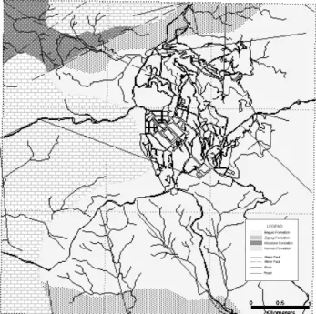
Fig. 1. Study area

Fig. 1. Study area.

Refice and Capolongo, 2002; Carro et al., 2003; Shou and Wang, 2003; Zhou et al., 2003). As a new approach to land-slide hazard evaluation using GIS, data mining using fuzzy logic, and artificial neural network models have been applied

Fig. 2. Geological Map

20

Fig. 2. Geological Map.

(Ercanoglu and Gokceoglu, 2002; Pistocchi et al., 2002; Lee et al., 2003a, b, 2004b).

2 Study area

Terramont Foundation (1992) stated that within the study area of Baguio City, development presently continues with-out the benefit of a working extant land use plan. This has resulted in the creation of an uncontrolled urban sprawl, with a proliferation of squatter colonies on both private and public land, and a high population density reflected in an overcrowded city experiencing increasingly mixed urban land use. Most development involves massive movement of ground within and beyond feasible construction areas, giving rise to possible erosion, floods and landslide hazards.

The study area (Fig. 1) lies within 16◦2300000–16◦2900000 latitude and 120◦3400000–120◦3700000 longitude It is located along the main trace and splays of the Philippine Fault which is a major seismic feature. Of particular interest are the northwest–southeast trending splays of this structure that are the western Tuba Fault and the Tebbo Fault to the east. Both of these faults are located less than 5 km. away from the city center (Pinet and Stephan, 1990).

Geology plays an important role in landslide potential, and the composition of the study area (Fig. 2) was taken from the work of PINA (1994) and David (1997). Four formations occur, and these are from the base:

(1) Zigzag Formation: conglomerate, sandstone and some limestone lenses.

(4)

(2) Kennon Formation: principally massive biohermal limestone, calcarenite and calcirudite. The basal por-tion consists of wacke, conglomeratic calcarenite with volcanic diorite pebble and cobble clasts.

(3) Klondyke Formation: clastic sedimentary rock consist-ing mainly of polymictic conglomerate with interbed-ded sandstone, siltstone and shale and in places interca-lated with flow breccia and pyroclastic rock. It rests un-conformably upon the Kennon Limestone and underlies wide areas on the elevated western side of the Baguio City Quadrangle.

(4) Baguio Formation: tuff, volcanic conglomerate and breccia, glassy and porphyritic andesite, with minor sandstone layers.

3 Ground acceleration map

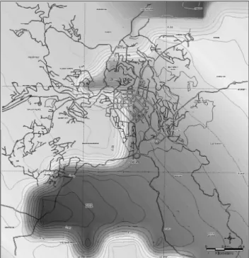
To verify and compare the landslide-susceptibility maps, the existing ground acceleration map (Fig. 3) was used. Al-though ground-motion hazard studies for the Philippines were made (Tenhaus et al., 1994) after the 1990 Baguio earthquake, the maps produced for peak horizontal ground acceleration are regional in scope and probabilistic in nature. Consequently, ground acceleration maps using a more deter-ministic approach have been employed. These engage the re-cent attenuation equation of Fukushima and Tanaka (1990). The relation is as follows:

Log10A = 0.41M − log 10(R + 0.032 × 100.41M) − 0.0034R + 1.30 (1) where A is the mean peak acceleration (in cm/s2), R is the shortest distance between the site and fault rupture (km) and M is the magnitude of the earthquake.

The equivalent ground acceleration in terms of gravity, g, is computed using the equation:

g = A/(980 cm/s2). (2) In assessing the distance R in Eq. (1), both the Tuba and Tebbo faults were regarded as seismic sources. R in Eq. (1) is the shortest distance measured from a grid point to either the Tuba or Tebbo fault trace, whichever is the shorter mea-surement of the two. The final g value in the map is further controlled by the geology in the area. The Baguio Forma-tion is assigned here as the rock medium of slip. The Zigzag, Klondyke and Kennon formations are classified as hard rock, with a correction factor of 0.6 in considering the final g. The highest value computed for the grid points is 0.634092 g and this lies within the Baguio Formation. The lowest value de-rived is 0.3366503 from the Zigzag Formation.

4 Artificial neural network and weight determination An artificial neural network is a “computational mechanism able to acquire, represent, and compute a mapping from one

Fig. 3. Ground acceleration map

21 Fig. 3. Ground acceleration map.

multivariate space of information to another, given a set of data representing that mapping” (Garrett, 1994). The back-propagation training algorithm is the most frequently used neural network method and is the method used in this study. The back-propagation training algorithm is trained using a set of examples of associated input and output values. The purpose of an artificial neural network is to build a model of the data-geneweight process, so that the network can general-ize and predict outputs from inputs that it has not previously seen. This learning algorithm is a multi-layered neural net-work, which consists of an input layer, hidden layers, and an output layer. The hidden and output layer neurons process their inputs by multiplying each input by a corresponding weight, summing the product, and then processing the sum using a nonlinear transfer function to produce a result. An artificial neural network “learns” by adjusting the weights between the neurons in response to the errors between the actual output values and the target output values. At the end of this training phase, the neural network provides a model that should be able to predict a target value from a given input value.

There are two stages involved in using neural network for multi-source classification: the training stage, in which the internal weights are adjusted; and the classifying stage. Typ-ically, the back-propagation algorithm trains the network un-til some targeted minimal error is achieved between the de-sired and actual output values of the network. Once the train-ing is complete, the network is used as a feed-forward struc-ture to produce a classification for the entire data (Paola and Schwengerdt, 1995).

(5)

22

Fig. 4. Architecture of neural network for ground subsidence hazard analysis.

Slope Aspect Curvature Distance from drainage Geology Distance from fault Land Cover Terrain mapping unit

Factor Input Hidden

Oi

Output

Ok

Landslide Non prone area

Landslide prone area Wjk Wij j=16 j=1 j=2 j=3 • • • • • • • • • •

Fig. 4. Architecture of neural network for ground subsidence

haz-ard. analysis.

A neural network consists of a number of interconnected nodes. Each node is a simple processing element that re-sponds to the weighted inputs it receives from other nodes. The arrangement of the nodes is referred to as the network architecture (Fig. 4). The receiving node sums the weighted signals from all the nodes that it is connected to in the pre-ceding layer. Formally, the input that a single node receives is weighted according to Eq. (3).

netj =

X

i

wij ·oi (3)

where wijrepresents the weights between nodes i and j , and

oi is the output from node j , given by

oj =f (netj). (4)

The transfer function f is usually a non-linear sigmoid func-tion that is applied to the weighted sum of inputs before the signal propagates to the next layer. One advantage of a sig-moid function is that its derivative can be expressed in terms of the function itself:

f0(netj) = f (netj)(1 − f (netj)) (5)

The network used in this study consisted of three layers. The first layer is the input layer, where the nodes were the ele-ments of a feature vector. The second layer is the internal or “hidden” layer. The third layer is the output layer that presents the output data. Each node in the hidden layer is interconnected to nodes in both the preceding and follow-ing layers by weighted connections (Atkinson and Tatnall, 1997).

The error, E, for an input training pattern, t , is a function of the desired output vector, d, and the actual output vector,

o, given by: E = 1 2 X k (dk−ok). (6)

The error is propagated back through the neural network and is minimized by adjusting the weights between layers. The weight adjustment is expressed as:

wij(n +1) = η(δj·oi) + α1wij (7)

where η is the learning rate parameter (set to η=0.01 in this study), δj is an index of the rate of change of the error, and

αis the momentum parameter (set to α=0.01 in this study). The factor δjis dependent on the layer type. For example,

for hidden layers, δj =(

X

δkwj k)f0(netj) (8)

and for output layers, δj =(dk−ok)f0(netk) (9)

This process of feeding forward signals and back-propagating the error is repeated iteratively until the error of the network as a whole is minimized or reaches an acceptable magnitude.

Using the back-propagation training algorithm, the

weights of each factor can be determined and may be used for classification of data (input vectors) that the network has not seen before. Zhou (1999) described a method for deter-mining the weights using back propagation. From Eq. (4), the effect of an output, oj, from a hidden layer node, j , on

the output, ok, from an output layer (node k) can be

repre-sented by the partial derivative of okwith respect to ojas

∂ok ∂oj =f0(netk) · ∂(netk) ∂oj =f0(netk) · wj k. (10)

Equation (10) produces both positive and negative values. If the effect’s magnitude is all that is of interest, then the im-portance (weight) of node j relative to another node j 0 in the hidden layer may be calculated as the ratio of the abso-lute values derived from Eq. (10):

|∂ok| ∂oj .|∂o_k| ∂oj0 = f0(netk) · wj k f0₍_net k) · wj0k = wj k wj0k . (11)

We should mention that wj0kis simply another weight in wj k

other than wik.

For a given node in the output layer, the results of Eq. (11) show that the relative importance of a node in the hidden layer is proportional to the absolute value of the weight necting the node to the output layer. When the network con-sists of output layers with more than one node, then Eq. (11) cannot be used to compare the importance of two nodes in the hidden layer.

wj0k= 1 J · J X j =1 wj k (12) tj k = wj k 1 J · J P j =1 wj k = J · wj k J P j =1 wj k (13)

(6)

Therefore, with respect to node k, each node in the hidden layer has a value that is greater or smaller than unity, de-pending on whether it is more or less important, respectively, than an average value. All the nodes in the hidden layer have a total importance with respect to the same node, given by

J

X

j =1

tj k =J. (14)

Consequently, the overall importance of node j with respect to all the nodes in the output layer can be calculated by

tj = 1 K · K X j =1 tj k. (15)

Similarly, with respect to node j in the hidden layer, the nor-malized importance of node j in the input layer can be de-fined by sij = wij 1 I · I P i=1 wij = I · wij I P i=1 wij . (16)

The overall importance of node i with respect to the hidden layer is si = 1 J · J X j =1 sij. (17)

Correspondingly, the overall importance of input node i with respect to output node k is given by

sti = 1 J · J X j =1 sij·tj. (18)

5 Data and methodology

Data preparation involved the digitization or creation of a GIS database which included the topographical, geomorpho-logical, geological and land cover data. A digitized map of earthquake-induced landslide locations detected from satel-lite imagery and field survey was produced, and these dig-ital data were included in the GIS. A vector-to-raster con-version was undertaken to provide raster data of landslides. The factors of slope, aspect, curvature, proximity to drainage, lithology, proximity to faults, land cover and geomorpho-logic/terrain units were used.

Contour and survey base points that had an elevation value read from the 1:10 000 scale topographic map were extracted and a Digital Elevation Model (DEM) was constructed. Us-ing the DEM, the slope gradient, slope aspect and curvature were calculated. The slope gradient of a surface refers to the maximum rate of change in z values across a region of the surface and the slope aspect is the compass direction max-imum rate of change in z in a downward direction. The

curvature represents the morphology of the topography. A positive curvature indicates that the surface is upwardly con-vex in that cell, and a negative shows that the surface is up-wardly concave. A zero value represents a flat surface. The distance from drainage was calculated in 1 m intervals. The land use/land cover data were derived from the 1:10 000 to-pographic map.

The lithology was taken from the 1:50 000 scale geolog-ical map, and the distance from a lineament was measured to the nearest 1 m interval. Distance buffers on both sides of a fault were generated to note the occurrence of landslides with respect to fault lines. Most of the landslides that oc-curred following the 1990 earthquake were observed to be within the 500 m buffer.

Landslides occur in varying terrain units, which are flood-plain, deep, wide or shallow valleys, basin, plateau, karst, or limestone hills. Floodplain is cultivated flat terrain. Pro-nounced meanders occur in narrow, deep valleys with wide drainage divides. Wide valley is a broad valley with a nar-row floodplain dominated by active erosion processes. Shal-low valley is characteristically narrow and shalShal-low with steep slopes in generally rugged terrain. Basin is a shallow de-pression with rounded contours and poor development of drainage lines. Plateau is well-drained round ridges and peaks dominated by narrow plateaus rather than valleys. Karst is rugged terrain characterized by sinkholes and poorly defined drainage lines. Limestone hills are poorly drained, with rounded contours and an absence of sinkholes.

The study area was divided into a grid with 10 m×10 m cells, occupying 560 rows and 541 columns in all total-ing 295 637 grid cells and earthquake-induced landslides oc-curred in 61 of these.

Maps relevant to the landslide occurrences were used first to construct a vector-type spatial database using the ARC/INFO GIS software package. Secondly, landslide oc-currence areas were detected during field survey of the study area. A map of the landslide locations was made as part of the GIS spatial database. Thirdly, for their weight determi-nation, the landslide factors were entered into an ARC/INFO grid type, and then converted to ASCII data for use with an artificial neural network program.

The results of the analysis were converted to grid data us-ing the GIS. For detected landslide location, the weight of each factor was determined by a neural network method. de-veloped using MATLAB (Hines, 1997). For factor weight determination using this approach, the ground subsidence lo-cation was assigned as an experiment area. When the weights converged to a proper value, they were determined by back

propagation between the neural network layers. Finally,

ground subsidence hazard mapping was carried out consider-ing the factor weight derived from our study, and the analyt-ical results were verified in a comparison with ground subsi-dence locations. In this study, the GIS software ArcView 3.3 and ARC/INFO version 9.0 were used as the basic analysis tools for spatial management and data processing.

(7)

Select Training sets

Collect GIS DB

Select Neural Networks Architecture

Select Neural Networks Architecture Weight Interpretation Weight Interpretation Weight Determination of Ground Subsidence Weight Determination of Ground Subsidence RMS Goal Met? Change Weights or Increase NN Size Change Weights or Increase NN Size Initialize NN Weights Initialize NN Weights Iteration(10) no

Neural Networks Weights

Reselect Training Sets

Select Training sets

Collect GIS DB

Select Neural Networks Architecture

Select Neural Networks Architecture Weight Interpretation Weight Interpretation Weight Determination of Ground Subsidence Weight Determination of Ground Subsidence RMS Goal Met? Change Weights or Increase NN Size Change Weights or Increase NN Size Initialize NN Weights Initialize NN Weights Iteration(10) no

Neural Networks Weights

Fig. 5. The flow chart of neural network training for weight determination

Fig. 6. Backpropagataion training results

23

Fig. 5. The flow chart of neural network training for weight

deter-mination.

6 Landslide-susceptibility analysis using the artificial neural network

Landslide-prone occurrences from the 61 sites and locations without slide susceptibilities were selected as experiment sites using slope map and landslide location data. To assess the effect of the exercise site selection, they were identified as areas where differing slope values with a 5 degree inter-val were classified as “areas not prone to landslides”, and ar-eas of landslides were assigned as “arar-eas prone to landslides” sets. If the analysis selected more than 61 sites with the same value then the sites were chosen at random.

The back-propagation algorithm was applied to calculate the weights between the input and hidden layers, and be-tween the hidden and output layers, by modifying the num-ber of hidden nodes and the learning rate. A three-layered feed-forward network was established using the MATLAB software package based on the framework provided by Hines (1997) in which “feed-forward” denotes that the interconnec-tions between the layers propagate forward to the next layer. The number of hidden layers and the number of nodes in such a layer required for a particular classification problem are not easy to deduce. In this study, an 8×16×2 structure was selected for the network with input data normalized in the range 0.1–0.9. The nominal and interval class group data were converted to continuous values ranging between 0.1 and 0.9. Continuous values were not, therefore, ordinal, but nom-inal data, and the numbers denote the classification of the in-put data. The learning rate was set to 0.01, and the initial weights were randomly selected to values between 0.1 and 0.3.

The back-propagation algorithm was used to minimize the error between the predicted and calculated output values. The algorithm propagated the error backwards, and

itera-Select Training sets Select Training sets Collect GIS DB Collect GIS DB

Select Neural Networks Architecture Select Neural Networks

Architecture Weight Interpretation Weight Interpretation Weight Determination of Ground Subsidence Weight Determination of Ground Subsidence RMS Goal Met? Change Weights or Increase NN Size Change Weights or Increase NN Size Initialize NN Weights Initialize NN Weights Iteration(10) no

Neural Networks Weights Neural Networks Weights

Reselect Training Sets Select Training sets

Select Training sets Collect GIS DB Collect GIS DB

Select Neural Networks Architecture Select Neural Networks

Architecture Weight Interpretation Weight Interpretation Weight Determination of Ground Subsidence Weight Determination of Ground Subsidence RMS Goal Met? Change Weights or Increase NN Size Change Weights or Increase NN Size Initialize NN Weights Initialize NN Weights Iteration(10) no

Neural Networks Weights Neural Networks Weights

Fig. 5. The flow chart of neural network training for weight determination

Fig. 6. Backpropagataion training results

23

Fig. 6. Backpropagataion training results.

Table 1. Weights of each factor for each selection of training site.

Factor Weight Normalized

Weight

Slope (unit: degree) 0.2003 2.300

Aspect 0.1302 1.495

Curvature (Unitless) 0.1088 1.249

Distance from Drainage (unit: m) 0.1031 1.184

Geology 0.1278 1.467

Distance from Fault (unit: m) 0.0871 1.000

Land Cover 0.1033 1.186

Terrain mapping unit 0.1395 1.602

tively adjusted the weights. The number of epochs was set to 2000, and the root mean square error (RMSE) value used for the stopping criterion was set to 0.1. The experimen-tal data sets met the 0.1 RMSE goals in the case of 0 slope (Fig. 6). If the RMSE value was not achieved however, then the maximum number of iterations was terminated at 2000 epochs.

Figure 5 is the flowchart of the neural network exercise for weight determination. The weights between layers that ac-quired by using the neural network were calculated reversely and the contribution or importance of each factor was de-rived for each set in the exercise. With slope at 0, the fi-nal weights of the 8 factors used to predict landslide sus-ceptibility are shown in Table 1. For easy interpretation, the weight values were normalized. Distance from a fault has the minimum weight value of 1.00, and slope has the maximum value of 2.30. Finally, the weights were applied across the entire study area, and the landslide-susceptibility map was then developed (Fig. 7). Susceptibility was classified into four classes: highest 10%, second 10%, third 20% and re-mainder 60%, based on area for easy visual interpretation. The minimum value obtained was 0.0092 and 0.9971 was the maximum. The mean value is 0.3784 and the standard deviation 0.2534.

(8)

Fig. 7. Landslide susceptibility mapping using artificial neural network.

24

Fig. 7. Landslide susceptibility mapping using artificial neural

net-work.

7 Verification

Two basic assumptions are required in the verification of landslide-susceptibility calculation models. One is that land-slides are related to spatial factors such as topography, ge-ology and land cover, and the other is that future landslides will be triggered by a specific impact such as seismic shock or heavy rainfall (Brabb, 1984; Varnes, 1978). Both assump-tions are satisfied in this study because the landslides were related to spatial factors and were triggered by earthquake.

The susceptibility analysis result was verified using known landslide locations compared with the landslide-susceptibility map. Rate curves were created and areas under the curve were calculated in each case. The rate illustrates how well the model and factor predict landslide and, the area under the curve enables an assessment of the prediction ac-curacy qualitatively. To obtain the relative ranking for each prediction pattern, the calculated index values of all cells in the study area were sorted in descending order. The ordered cell values were divided into 100 classes, with accumulated 1% intervals. In Fig. 8, for slope 0 the rate verification re-sults appear as a line. However, the, 90 to 100% (10%) clas-sification of the study area where the landslide-susceptibility

0 10 20 30 40 50 60 70 80 90 100 0 10 20 30 40 50 60 70 80 90 100

Fig. 8. Illustration of cumulative frequency diagram showing landslide susceptibility index rank (x-axis) occurring in cumulative percent of landslide occurrence (y-(x-axis).

25

Fig. 8. Illustration of cumulative frequency diagram showing

land-slide susceptibility index rank (x-axis) occurring in cumulative per-cent of landslide occurrence (y-axis).

index had a higher rank accounts for 75% of all the land-slides. Furthermore, the 80 to 100% (20%) classification of the study area predicts 92% of the landslides.

To compare the result quantitatively the areas under the curve were recalculated with the total area as 1 which means perfect prediction accuracy. Consequently, the area under a curve can be used to assess the prediction accuracy qualita-tively. In the case of slope 0, the area ratio was revealed as 0.9320 and we can say that the prediction accuracy is thus 93.20%.

To assess the effect of experiment site selection locations, sites were chosen as areas where slope values with a 5◦ in-terval were classified as prone or not prone to landslides. Af-ter considering the slope, the verification showed that with a slope increase, the accuracy decreased (Table 2). Above 36◦, the prediction accuracy has a particularly low value. Because landslide is notably related to slope, the designation of such a test site as a “landslide not prone area” has an effect on the accuracy of a landslide-susceptibility map.

The landslide-susceptibility map was also visually com-pared with the ground acceleration map (Fig. 3). The land-slide possibility and ground acceleration values are higher in the south than elsewhere in the study area.

8 Discussion and conclusions

Landslides are among the most hazardous of natural disas-ters. Government and research institutions worldwide have attempted for years to assess landslide hazard and risk and to show its spatial distribution. In this study, a data bank approach by means of a GIS shows considerable promise in the identification of areas susceptible to landslide caused

(9)

Table 2. Verification result according to different training site

se-lection (different slope).

Slope value No. of Ratio No. of Ratio Frequency Area under (degree) total cell (%) landslide (%) ratio curve

0 32234 10.83 0 0.00 0.00 93.20 1–5 29602 9.95 0 0.00 0.00 92.88 6–10 52925 17.78 1 1.64 0.09 93.11 11–15 64294 21.61 0 0.00 0.00 92.91 16–20 50089 16.83 1 1.64 0.10 93.21 21–25 32852 11.04 10 16.39 1.48 93.10 26–30 19084 6.41 14 22.95 3.58 91.88 31–35 9551 3.21 9 14.75 4.60 84.31 36–40 4036 1.36 7 11.48 8.46 17.62 41–45 1406 0.47 13 21.31 45.11 11.54 46–50 465 0.16 3 4.92 31.47 13.94 51–55 197 0.07 2 3.28 49.53 15.28 56–60 177 0.06 0 0.00 0.00 14.36 61–65 191 0.06 0 0.00 0.00 20.05 66–70 212 0.07 0 0.00 0.00 14.16 71–75 119 0.04 0 0.00 0.00 16.13 76–81 151 0.05 1 1.64 32.31 18.03 Total 297585 100.00 61 100.00 1.00

by earthquakes. In the verification of landslide-susceptibility maps, the artificial neural network showed a very high

pre-diction accuracy of 93.20% in the case of 0 slope. The

landslide-susceptibility map was spatially consistent when compared with the ground acceleration.

The back-propagation algorithm presented difficulties when trying to follow the internal procedures. The method involves a long execution time, has a heavy computing load, and there is a requirement to convert the database to another format. Landslide susceptibility can, however, be analyzed qualitatively. In addition to using a multifaceted approach to a solution, the extraction of reliable results for a complex problem is possible with continuous and discrete data pro-cessing.

These results can be used as basic data to assist slope management and land-use planning. The models used in the study are valid for generalized assessment purposes, although they may be less useful at a site-specific scale where local geological and geographic heterogeneities may prevail.

Edited by: F. Guzzetti

Reviewed by: C. Gokceoglu and D. Keefer

References

Arboleda, R. A. and Regalado, M. T.: Inventory and characteriza-tion of landslides induced by the 16 July 1990 Luzon, Philippines Earthquake, 1990.

Atkinson, P. M., and Tatnall, A. R. L.: Introduction neural networks in remote sensing, International Journal of Remote Sensing, 18, 699–709, 1997.

Baeza, C. and Corominas, J.: Assessment of shallow landslide sus-ceptibility by means of multivariate statistical techniques, Earth

Surface Processes and Landforms, 26, 1251–1263, 2001. Brabb, E. E.: Innovative approach to landslide hazard and risk

map-ping. Proceedings of the 4th International Symposium on Land-slides, Toronto, pp. 307–324, 1984.

Carro, M., De Amicis, M., Luzi, L., and Marzorati, S.: The applica-tion of predictive modeling techniques to landslides induced by earthquakes: the case study of the 26 September 1997 Umbria-Marche earthquake (Italy), Eng. Geol., 69, 139–159, 2003. Clerici, A., Perego, S., Tellini, C., and Vescovi, P.: A procedure

for landslide susceptibility zonation by the conditional analysis method, Geomorphology, 48, 349–364, 2002.

Dai, F. C. and Lee, C. F.: Landslide characteristics and slope insta-bility modeling using GIS, Lantau Island, Hong Kong, Geomor-phology, 42, 213–228, 2002.

Dai, F. C., Lee, C. F., Li, J., and Xu, Z. W.: Assessment of landslide susceptibility on the natural terrain of Lantau Island, Hong Kong, Environ. Geol., 40, 381–391, 2001.

David Jr., S. D.: Morphological and Morphstructural Analysis of SW Central Cordillera Luzon, Philippine, 1997.

Donati, L. and Turrini, M. C.: An objective method to rank the im-portance of the factors predisposing to landslides with the GIS methodology: application to an area of the Apennines (Valner-ina; Perugia, Italy), Eng. Geol., 63, 277–289, 2002.

Ercanoglu, M. and Gokceoglu, C.: Assessment of landslide suscep-tibility for a landslide-prone area (north of Yenice, NW Turkye) by fuzzy approach, Environ. Geol., 41, 720–730, 2002. Fukushima, Y. and Tanaka, T.: A new attenuation relation for peak

horizontal acceleration of strong earthquake ground motion in Japan, Bulletin of Seismological Society of America, 80, 757– 777, 1990.

Garrett, J.: Where and why artificial neural networks are applicable in civil engineering, J. Comput. Civil Eng., 8, 129–130, 1994. Gokceoglu, C., Sonmez, H., and Ercanoglu, M.: Discontinuity

con-trolled probabilistic slope failure risk maps of the Altindag (set-tlement) region in Turkey, Eng. Geol., 55, 277–296, 2000. Guzzetti, F., Carrarra, A., Cardinali, M., and Reichenbach, P.:

Landslide hazard evaluation: a review of current techniques and their application in a multi-scale study, Central Italy, Geomor-phol., 31, 181–216, 1999.

Hines, J. W.: Fuzzy and Neural Approaches in engineering, John Wiley and Sons, Inc. New York, 210, 1997.

Jibson, R. W., Harp, E. L., and Michael, J. A.: A method for pro-ducing digital probabilistic seismic landslide hazard maps, Eng. Geol., 58, 271–289, 2000.

Lee, S. and Min, K.: Statistical analysis of landslide susceptibility at Yongin, Korea, Environ. Geol., 40, 1095–1113, 2001. Lee, S., Chwae, U., and Min, K.: Landslide susceptibility mapping

by correlation between topography and geological structure: the Janghung area, Korea, Geomorphol., 46, 49–162, 2002a. Lee, S., Choi, J., and Min, K.: Landslide susceptibility analysis

and verification using the Bayesian probability model, Environ. Geol., 43, 120–131, 2002b.

Lee, S. and Choi, U.: Development of GIS-based geological hazard information system and its application for landslide analysis in Korea, Geosci. J., 7, 243–252, 2003.

Lee, S., Ryu, J. H., Lee, M. J., and Won, J. S.: Landslide suscep-tibility analysis using artificial neural network at Boun, Korea, Environ. Geol., 44, 820–833, 2003a.

Lee, S., Ryu, J. H., Min, K. D., and Won, J. S.: Landslide

(10)

tibility analysis using GIS and artificial neural network, Earth Surface Processes and Landforms, 27, 1361–1376, 2003b. Lee, S., Choi, J., and Woo, I.: The effect of spatial resolution on

the accuracy of landslide susceptibility mapping: a case study in Boun, Korea, Geosci. J., 8, 51–60, 2004a.

Lee, S., Ryu, J. H., Won, J. S., and Park, H. J.: Determination and application of the weights for landslide susceptibility map-ping using an artificial neural network, Eng. Geol., 71, 289–302, 2004b.

Luzi, L., Pergalani, F., and Terlien, M. T. J.: Slope vulnerability to earthquakes at subregional scale, using probabilistic techniques and geographic information systems, Eng. Geol., 58, 313–336, 2000.

Ohlmacher, G. C. and Davis, J. C.: Using multiple logistic regres-sion and GIS technology to predict landslide hazard in northeast Kansa, USA, Eng. Geol., 69, 331–343, 2003.

Paola, J. D. and Schowengerdt, R. A.: A review and analysis of backpropagation neural networks for classification of remotely sensed multi-spectral imagery, Int. J. Remote Sens., 16, 3033– 3058, 1995.

Parise, M. and Jibson, R. W.: A seismic landslide susceptibility rat-ing of geologic units based on analysis of characteristics of land-slides triggered by the 17 January, 1994 Northridge, California earthquake, Eng. Geol., 58, 251–270, 2000.

Pi˜na, R. E.: Report on the geologic mapping of Baguio and Si-son Quadrangles, Mines and Geosciences Bureau, Quezon City, Philippines, 1994.

Pinet, N. and Stephan, J. F.: The Philippine wrench fault system in the Ilocos Foothills, Northwestern Luzon, Philippines, Tectono-physics, 183(1–4), 207–224, 1990.

Pistocchi, A., Luzi, L., and Napolitano, P.: The use of pre-dictive modeling techniques for optimal exploitation of spatial databases: a case study in landslide hazard mapping with expert system-like methods, Environ. Geol., 41, 765–775, 2002.

Rautelal, P. and Lakheraza, R. C.: Landslide risk analysis between Giri and Tons Rivers in Himachal Himalaya, India, International Journal of Applied Earth Observation and Geoinformation, 2, 153–160, 2000.

Refice, A. and Capolongo, D.: Probabilistic modeling of uncertain-ties in earthquake-induced landslide hazard assessment, Comput-ers & Geosciences, 28, 735–749, 2002.

Romeo, R.: Seismically induced landslide displacements: a predic-tive model, Eng. Geol., 58, 337–351, 2000.

Shou, K. J. and Wang, C. F.: Analysis of the Chiufengershan land-slide triggered by the 1999 Chi-Chi earthquake in Taiwan, Eng. Geol., 68, 237–250, 2003.

Tenhaus, P. C., Stanley, L. H., and Algernussen, S. T.: Estimates of the Regional Ground-Motion Hazard in the Philippines, in Natu-ral Disaster Mitigation in the Philippines (Proceedings), pp. 71– 98, 1994.

Terramont Foundation, I.: Feasibility study in the City Camp La-goon land recovery project: City Planning Office, 1992. Varnes, D. J.: Slope movement types and processes, landslides

anal-ysis and control. Special Report 176. Transportation Research Board, Washington, D.C., pp 11–80, 1978.

Zhou, G., Esaki, T., Mitani, Y., Xie, M., and Mori, J.: Spatial prob-abilistic modeling of slope failure using an integrated GIS Monte Carlo simulation approach, Eng. Geol., 68, 373–386, 2003. Zhou, C. H., Lee, C. F., Li, J., and Xu, Z. W.: On the spatial

relation-ship between landslides and causative factors on Lantau Island, Hong Kong, Geomorphol., 43, 197–207, 2002.

Zhou, W.: Verfication of the nonparametric characteristics of backpropagation neural networks for image classification, IEEE Trans., On Geoscience and Remote Sensing, 38, 771–779, 1999.