HAL Id: hal-01627085
https://hal.archives-ouvertes.fr/hal-01627085
Submitted on 31 Oct 2017
HAL is a multi-disciplinary open access
archive for the deposit and dissemination of
sci-entific research documents, whether they are
pub-lished or not. The documents may come from
teaching and research institutions in France or
abroad, or from public or private research centers.
L’archive ouverte pluridisciplinaire HAL, est
destinée au dépôt et à la diffusion de documents
scientifiques de niveau recherche, publiés ou non,
émanant des établissements d’enseignement et de
recherche français ou étrangers, des laboratoires
publics ou privés.
Supply planning optimization for linear production
system with stochastic lead-times and quality control
Oussama Ben-Ammar, Belgacem Bettayeb, Alexandre Dolgui
To cite this version:
Oussama Ben-Ammar, Belgacem Bettayeb, Alexandre Dolgui. Supply planning optimization for
lin-ear production system with stochastic lead-times and quality control. International Conference on
Industrial Engineering and Systems Management (IESM 2017), Oct 2017, Sarrebruck, Germany.
�hal-01627085�
Supply planning optimization for linear production system with stochastic lead-times and quality control (presented at the 7th IESM Conference, October 11 – 13, 2017, Saarbrücken, Germany)
O. Ben Ammar, B. Bettayeb, A. Dolgui SLP/LS2N – CNRS UMR 6004
Automation, Production and Computer Sciences Department. IMT Atlantique, Bretagne-Pays de la Loire, Campus Nantes, France {oussama.ben-ammar, belgacem.bettayeb, alexander.dolgui}@imt-atlatique.fr
Abstract— This work consider the problem of supply
planning optimization of imperfect production systems with stochastic lead times and quality control. A model for supply planning of the production system and three quality control policies are analyzed. Experimental results highlights the economic advantage of integrating quality control planning at the early phase of supply planning optimization of production systems.
Keywords—Imperfect production systems; Uncertainty; Linear chain production process; Quality control.
I. Introduction and related publications
The growing need for more flexible and responsive production systems leads to several new approaches aiming to endow the production systems of the future with a certain intelligence, agility and resilience. In this context, one of the most important challenges to deal with is uncertainty and its impact on the performances of the system. In fact, uncertainty causes to manufacturers several difficulties in planning production, in regulating inventory, and in meeting demand [1]. In the following, the serial supply chain structures with stochastic lead times are reviewed. We present the case of deterministic demand for one and multilevel serial supply chains. Then, we focus on some relevant works related to production planning integrating quality control.
The simulation study presented by Whybark and Williams [2] was among the first to suggest that safety lead times may perform better than safety stocks in a multi-level linear production-inventory system when the production and replenishment times are stochastic.
A few years later, Weeks [3] proposed a one-stage model where it is assumed a deterministic demand, a stochastic processing time and tardiness and holding costs. This problem has been proved to be equivalent to the standard “Newsboy” formulation.
Another analytical approach is proposed by Yano [4] to model serial production systems in order to optimize the planned lead times. In this model, which is based on a Lot-for-Lot (L4L) policy, it is assumed that procurement and processing times are stochastic and demand is deterministic. The objective function is composed of the holding and tardiness costs. A procedure is developed to generate solutions for two-stage systems. The same author extended this model to three-stage systems in [5]. In this
model, a replenishment cost is introduced each time a given component is available after a planned intermediary due date. The performance indicator to be minimized is the sum of the following costs: i) the expected holding and tardiness costs at each stage, and ii) the expected tardiness cost for the finished product. The author underlined the difficulty to model a system composed of more than three stages. It is only after many year that Elhafsi [6] overcome this barrier by proposing an analytical model based on recursivity. The convexity of the objective function is proved and a dynamic programming based heuristic is proposed to find approximate solutions of good quality in an acceptable computer processing time.
In inventory control process, Kim et al. [7] consider one product, a known fixed demand and an Erlang-distributed lead times. The performance indicator is the expected total cost, which is composed of ordering, holding and tardiness costs. Based on the analytical formulation, the authors propose an approximate solution and compare it to optimal ones for the case where the prior information on the lead time distribution is available, and another case where no information exists. The results show the effectiveness and the robustness of this approach and how costs could be reduced under uncertain lead times. Two years later, Kim et al. [8] studied the same problem and analysed the bullwhip effect which is encountered when both demand and lead times are stochastic. An analytical method is used to prove that prior information on lead times variability could be very helpful to control the bullwhip effect in a multi-stage supply chain.
Apparently, the literature contains few publications considering linear chain supply planning with discrete lead times. The most of existing studies investigates the lead time uncertainty for one item or assembly systems. Readers can refer to [9], [10] and [11] where more complete literature reviews are provided concerning supply planning dealing with uncertainty on lead times. For other sources of uncertainty (demand, capacity, cost, etc.) readers can refer to the surveys of Aloulou et al. [12] and Díaz-Madroñero et al. [13].
In the last few decades, there has been a growing interest in integrating quality control in supply and production planning. In fact, the quality should be rigorously checked before delivering the finished product. In this way, the company ensures customer satisfaction and avoid excessive product returns. Nevertheless, it will be necessary to find a good compromise between the inspection costs and the cost of non-conformity. In this regard, Colledani and Tolio [14] investigate the interaction between
quality control system and production system and show how they impact each other’s performances. They underline the necessity of jointly considering quality and logistics requirements while designing a production system.
The work of Rosenblatt and Lee [15] studies the relationship and the economic impact of the interaction between production planning, quality of products and the deterioration of the production process. The considered production process has two possible states in which it generates different rates of defectives. The objective is to determine the economic production quantities of this kind of production process while minimizing the total annual cost. The optimal production run time is determined for two deterioration models and multi-state deterioration.
Recently, Bettayeb et al. [16] proposed an integrated model for single item lot sizing and quality control planning. The objective is to minimize the total cost while ensuring a given level of outgoing quality. This cost is composed of holding, setup, production and inspection costs.
In the field of supply planning and quality control few papers analyses the uncertainty of lead time and quality control. In this work, we propose a model of supply planning optimization of imperfect production systems with stochastic lead times and quality control. The rest of the paper is organized as follows. The problem description and the general assumptions are described in the second section. The third one details the analytical models corresponding to three different quality control policies and the optimization approach. Section 4 presents the experimental results, compares the economical performances of each model and analysis the effects of some parameters. The paper ends by giving the conclusion and the perspectives of this work.
II. Problem description and assumptions
The problem under consideration in this paper concerns the optimization of supply planning of an imperfect linear production process where the lead times of the production steps are stochastic. The objective is to evaluate the effect of quality issues on the total cost of such a system and analyze the opportunity of integrating quality control activities in the optimization model of the system.
Before detailing the problem and the general assumptions, the following are the notations used in next sections. All costs are expressed in monetary unit and durations are expressed in time units.
Parameters
𝐶𝑃 Production cost
𝑐𝑖 Unit inspection cost
𝑐𝑛𝑐 Unit non-conformity cost
𝐶𝑄 Quality cost: the sum of inspection and non-conformity
costs
𝑆𝑅 Sampling rate, i.e. proportion of products inspected 𝑐ℎ Unit inventory holding cost per time unit
𝑐𝑡 Unit tardiness penalty per time unit
𝑇 Due date
𝑞0 Proportion of non-conforming finished products
generated by the whole production process. 𝑚 Number of production operations (flowshop)
𝐿𝑗 Lead time of operation 𝑗, ∀𝑗 ∈ {1,2, … , 𝑚} 𝐿𝑗 is a
discrete random variable which varies between 𝑙𝑗 and
𝑢𝑗
𝑡𝑖 Unit inspection duration
𝐿 Total lead time, i.e. 𝐿 = ∑𝑚𝑗=1𝐿𝑗
Decision variables
𝑋 Order release date
Functions
𝐸⟦. ⟧ Expected value of ⟦. ⟧
𝐹𝑚(. ) Cumulative distribution function of 𝐿
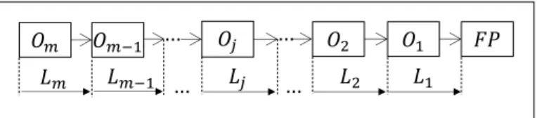
The considered production process is composed of 𝑚 process operations (Fig. 1), which are consecutively executed to obtain the finished product 𝐹𝑃. Each process step 𝑗 has a random lead time duration 𝐿𝑗. The product starts to be processed at time
𝑋 and the fished product is available at 𝑇𝑃𝐹= 𝑋 + 𝐿, after
accumulating the 𝑚 random lead times 𝐿 = 𝐿1+ 𝐿2+ ⋯ + 𝐿𝑚.
Note that 𝑇𝑃𝐹 is a random variable because of the randomness
of the total lead time 𝐿.
Apart from the processing cost (omitted here), and depending on the due date 𝑇 and the effective release date of the finished product, the generated production cost either equals the holding cost, if the product is finished before the due date, equals the tardiness penalty if it is available after the due date or equals zero if it is finished just in time.
Fig. 1. Linear production process
III. Analytical models and optimization approach This section contains three models each of them corresponds to a certain policy regarding the quality control. In the first case, only the non-conformity penalty is assumed and no quality control is performed. In the second case, the quality control is performed at the end of production process but only the lead times are taken into account in the supply and production planning. In the last case, the quality control and the lead time variability are both taken into account while optimizing the supply and production planning.
A. Reference Policy (𝜋0): No quality control
It corresponds to the case where no quality control is performed during the production process. However, for each non-conforming product delivered to the customer, the producer pays a non-conformity penalty. The total cost is composed of inventory holding cost, tardiness cost and non-conformity cost:
...
... ... ...
𝑇𝐶0(𝑋, 𝐿) = 𝐶
𝑃0+ 𝐶𝑄0 (1)
Where 𝐶𝑃0 is equal to the sum of 𝐶𝐻 the inventory holding
cost and 𝐶𝑇 the tardiness cost:
If the finished products are available before 𝑇, it will be stored. The corresponding inventory holding cost 𝐶𝐻 is equal to:
𝐶𝐻= 𝑐ℎ× (𝑇 − 𝑚𝑖𝑛(𝑇; 𝑋 + 𝐿)) (2)
There will be a stockout of the finished products if they are delivered after the due date 𝑇. Then tardiness cost 𝐶𝑇 is equal to:
𝐶𝑇= 𝑐𝑡× (𝑚𝑎𝑥(𝑇; 𝑋 + 𝐿) − 𝑇) (3)
And the non-conformity penalty 𝐶𝑄0 is equal to 𝑞0× 𝑐𝑛𝑐.
The total cost 𝑇𝐶0(𝑋, 𝐿) is a discrete random variable because of the randomness of the lead times 𝐿𝑗. Each of the latter
varies between 𝑙𝑗 and 𝑢𝑗, so the total cost has a finite number of
possible values.
Fig. 2. Quality control policies
Proprety 1. The expression of the expected value of the total cost,
denoted by 𝐸⟦𝑇𝐶0(𝑋, 𝐿)⟧, is given bellow:
𝐸⟦𝑇𝐶0(𝑋, 𝐿)⟧ = 𝑐 ℎ× (𝑇 − ∑ (1 − 𝐹𝑚(𝑠 − 𝑋)) 0≤𝑠≤𝑇−1 ) +𝑐𝑡× ∑(1 − 𝐹𝑚(𝑠 − 𝑋)) 𝑠≥𝑇 + 𝑞0× 𝑐 𝑛𝑐 (4)
Proof. From expressions (1), (2) and (3), we have:
𝐸⟦𝑇𝐶0(𝑋, 𝐿)⟧ = 𝐸⟦𝐶
𝑃0(𝑋, 𝐿)⟧ + 𝑞0× 𝑐𝑛𝑐
= 𝑐ℎ× (𝑇 − 𝐸⟦𝑚𝑖𝑛(𝑇; 𝑋 + 𝐿)⟧)
+𝑐𝑡× (𝐸⟦𝑚𝑎𝑥(𝑇; 𝑋 + 𝐿)⟧ − 𝑇) + 𝑞0× 𝑐𝑛𝑐
Let 𝛤 a positive discrete random variable (with a finite range). Its expected value can be expressed as follows:
𝐸⟦Γ⟧ = ∑(1 − 𝑃𝑟⟦𝛤 ≤ 𝑠⟧)
𝑠≥0
= ∑(1 − 𝐹𝛤(𝑠)) 𝑠≥0
(5) Knowing that 𝑋 + 𝐿 does not depend on 𝑇, and using expression (5), we get:
𝐸⟦𝑚𝑎𝑥(𝑇; 𝑋 + 𝐿)⟧ = ∑(1 − 𝑃𝑟⟦𝑇 ≤ 𝑠⟧ × 𝑃𝑟⟦𝑋 + 𝐿 ≤ 𝑠⟧)
𝑠≥0
Moreover, knowing that 𝑃𝑟⟦𝑇 ≤ 𝑠⟧ = 0 for all 0 ≤ 𝑠 < 𝑇, then: 𝐸⟦𝑚𝑎𝑥(𝑇; 𝑋 + 𝐿)⟧ = 𝑇 + ∑(1 − 𝑃𝑟⟦𝑋 + 𝐿 ≤ 𝑠⟧) 𝑠≥𝑇 = 𝑇 + ∑(1 − 𝐹𝑚(𝑠 − 𝑋)) 𝑠≥𝑇 (6)
Where 𝐹𝑚 is the cumulative distribution function of the total
lead time 𝐿, which defined as bellow: For 𝛼 = 0: 𝐹𝑚(𝑠 − 𝑋) = 𝑃𝑟⟦𝑋 + 𝐿𝑚≤ 𝑠⟧ For 1 ≤ 𝛼 ≤ 𝑚 − 1; 𝑚′= 𝑚 − 𝛼 : 𝐹𝑚′(𝑠 − 𝑋) = ∑ 𝑃𝑟⟦𝐿𝑚′= 𝑢𝛼⟧ × 𝐹𝑚′+1(𝑣𝛼− 𝑋) 𝑢𝛼+𝑣𝛼=𝑠 𝑢𝛼+𝑣𝛼∈ℤ
In the same way, we can easily deduce that: 𝐸⟦𝑚𝑖𝑛(𝑇; 𝑋 + 𝐿)⟧ = ∑ (1 − 𝐹𝑚(𝑠 − 𝑋))
0≤𝑠≤𝑇−1
∎ (7) The expected total cost (4) is the objective function. It is a non-linear function which should be minimized. An exact method based on Newsboy formula is used to solve this problem in polynomial time.
Proposition 1. The method based on Newsboy formula presented
in [17] gives the optimal order release date of the reference case
𝑋0∗: 𝐹𝑚(𝑇 − 𝑋0∗− 1 ) ≤ 𝑐𝑡 𝑐ℎ+ 𝑐𝑡≤ 𝐹𝑚(𝑇 − 𝑋0 ∗ ) (8)
Where 𝐹𝑚(. ) is the cumulative distribution function of the
total lead time 𝐿.
B. Policy 1 (𝜋1): Separated afterwards quality control
planning
In this case, we suppose that the quality inspection is done just after the production process. A proportion of finished products is randomly sampled and inspected. The non-conforming products detected by inspection are repaired with no-extra cost.
The total cost is composed of production and quality costs, denoted by 𝐶𝑃1 and 𝐶𝑄1, respectively.
𝑇𝐶1(𝑋, 𝐿, 𝑆𝑅) = 𝐶
𝑃1+ 𝐶𝑄1 (9)
a) Without Quality control performed by the produced (policy 𝜋0)
b) With quality control performed by the producer (Policies 𝜋1and 𝜋2 )
... ... Customer Producer S? ... ... OK? Customer Producer
Note that, in this case, 𝐶𝑃1 is the real production cost. It is equal to 𝐶𝑃0∗− ∆ℎ+ Δ𝑡, where:
𝐶𝑃0∗ is the optimal planned production cost associated to
optimal order release date 𝑋0∗,
∆ℎ is the holding cost reduction corresponding to the time
the product is being inspected :
∆ℎ= 𝑐ℎ× 𝑚𝑎𝑥(𝑚𝑖𝑛(𝐼; 𝑇 − 𝑋 − 𝐿); 0) (10)
Where 𝐼 = 𝑖𝑢× 𝑆𝑅 corresponds to the total duration of
inspection that corresponds to the quality control strategy in place.
Δ𝑡 is the tardiness cost increase due to the product inspection :
Δ𝑡= 𝑐𝑡× (𝐼 − 𝑚𝑎𝑥(𝑚𝑖𝑛(𝐼; 𝑇 − 𝑋 − 𝐿); 0)) (11)
The quality cost 𝐶𝑄1 is composed of the cost of inspection and
the penalty paid by the producer to the customer for non-conforming units:
𝐶𝑄1= 𝑞0× (1 − 𝑆𝑅) × 𝑐𝑛𝑐+ 𝑆𝑅 × 𝑐𝑖
As in the previous case, the total cost is also a random discrete random variable with a finite range. The expected cost is derived by the following property.
Proprety 2. The expression of the expected value of the total cost,
denoted 𝐸⟦𝑇𝐶1(𝑋0∗, 𝐿, 𝑆𝑅)⟧, is given bellow:
𝐸⟦𝑇𝐶1(𝑋 0∗, 𝐿, 𝑆𝑅)⟧ = 𝐸⟦𝑇𝐶0(𝑋0∗, 𝐿)⟧ − [(𝑐ℎ+ 𝑐𝑡) × ∑ 𝐹𝑚(𝑇 − 𝑠 − 1 − 𝑋0∗) 𝑠≤𝐼−1 − 𝑐𝑡× 𝐼] −𝑆𝑅 × (𝑐𝑛𝑐× 𝑞0− 𝑐𝑖)
Proof. From expression (4) and (7), 𝐸⟦𝑇𝐶0(𝑋0∗, 𝐿)⟧ can be
easily calculated. From expressions (10) and (11), we can easily deduce that:
𝐸⟦∆ℎ− Δ𝑡⟧ = ∑ 𝐹𝑚(𝑇 − 𝑠 − 1 − 𝑋0∗) 𝑠≤𝐼− 1
∎ C. Policy 2 (𝜋2): Integrated production and quality control
planning
In this case, we suppose that the quality control is planned in advance. It is made after the production process. A proportion of finished products is randomly sampled and inspected. The non-conforming products detected by inspection are repaired with no-extra cost.
The total cost is composed of production and quality costs, denoted by 𝐶𝑃2 and 𝐶𝑄2, respectively.
𝑇𝐶2(𝑋, 𝐿, 𝑆𝑅) = 𝐶 𝑃2+ 𝐶𝑄2 (12) Where: 𝐶𝑃2= [𝑐ℎ× (𝑇 − 𝑚𝑖𝑛(𝑇; 𝑋 + 𝐿 + 𝐼)) + 𝑐𝑡 × (𝑚𝑎𝑥(𝑇; 𝑋 + 𝐿 + 𝐼) − 𝑇)] 𝐶𝑄2= 𝑞0× (1 − 𝑆𝑅) × 𝑐𝑛𝑐+ 𝑆𝑅 × 𝑐𝑖
The total cost 𝑇𝐶2(𝑋, 𝐿, 𝑆𝑅) is a discrete random variable because of the randomness of lead times 𝐿𝑗. Each of the latter
varies between 𝑙𝑗 and 𝑢𝑗. Therefore, this total cost has a finite number of possible values. Thus, the mathematical expectation of cost can be determined.
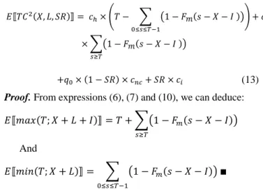
Proprety 1. The expression of the expected value of the total cost,
noted 𝐸⟦𝑇𝐶0(𝑋, 𝐿)⟧, is given bellow:
𝐸⟦𝑇𝐶2(𝑋, 𝐿, 𝑆𝑅)⟧ = 𝑐 ℎ× (𝑇 − ∑ (1 − 𝐹𝑚(𝑠 − 𝑋 − 𝐼 )) 0≤𝑠≤𝑇−1 ) + 𝑐𝑡 × ∑(1 − 𝐹𝑚(𝑠 − 𝑋 − 𝐼 )) 𝑠≥𝑇 +𝑞0× (1 − 𝑆𝑅) × 𝑐𝑛𝑐+ 𝑆𝑅 × 𝑐𝑖 (13)
Proof. From expressions (6), (7) and (10), we can deduce:
𝐸⟦𝑚𝑎𝑥(𝑇; 𝑋 + 𝐿 + 𝐼)⟧ = 𝑇 + ∑(1 − 𝐹𝑚(𝑠 − 𝑋 − 𝐼)) 𝑠≥𝑇 And 𝐸⟦𝑚𝑖𝑛(𝑇; 𝑋 + 𝐿)⟧ = ∑ (1 − 𝐹𝑚(𝑠 − 𝑋 − 𝐼)) 0≤𝑠≤𝑇−1 ∎
Proposition 2. The method based on Newsboy formula presented
in [17] gives the optimal order release date of the reference case
𝑋2∗:
𝐹𝑚(𝑇 − 𝑋2∗− 1 − 𝐼 ) ≤
𝑐𝑡
𝑐ℎ+ 𝑐𝑡≤ 𝐹𝑚(𝑇 − 𝑋2
∗− 𝐼) (14)
Where 𝐹𝑚(. ) is the cumulative distribution function of the
total lead time 𝐿.
IV. Numerical example and discussion
The proposed cases described in Section 3 have been coded in C++. The experiments are carried on computer with 2.32 GHz Intel core i7 and 8 GB of RAM memory.
A. Experiments setting
The experiments are based on an example of a linear production system with three production steps, i.e. 𝑚 = 3. The due date 𝑇 is equal to 20 and the lead time of each process step is a discrete random variable uniformly distributed over the range of integers from 1 to 5, i.e. Pr(𝐿𝑗= 𝑙) = 0.2 ∀𝑗 = 1,2,3 ∀𝑙 =
1,2, … , 5. It is assumed that the system is operating in a steady state, generating a constant proportion of non-conforming finished products 𝑞0= 0.05. The unit holding cost 𝑐ℎ is equal
to the monetary unit and the other cost parameters experimented are given in Table 1.
Table 1. Experimented values for each parameter
Parameter Range
𝐿𝑗 [1, 5]
𝜌𝑡= 𝑐𝑡/𝑐ℎ {0.1, 1, 10, 100,1000}
𝜌𝑖= 𝑐𝑖/𝑐ℎ {0.1, 1, 10, 100,1000}
𝑆𝑅 {0, 0.2, 0.4, … , 1} B. Results and discussions
The preliminary results presented in this section aim to analyze the effect of integrating quality control in the early stage of supply and production planning. To do so, the following notion are introduced:
The gap between policy 𝜋1 and policy 𝜋3
𝐺𝐴𝑃1 (%) = 100 ×𝐸𝑇𝐶1− 𝐸𝑇𝐶3 𝐸𝑇𝐶1
The gap between policy 𝜋2 and policy 𝜋3
𝐺𝐴𝑃2 (%) = 100 ×𝐸𝑇𝐶
2− 𝐸𝑇𝐶3
𝐸𝑇𝐶2
Figure 3 shows the variation of 𝐺𝐴𝑃1 as function of the cost of non-conformity for different values of sampling rate and for three values of the inspection cost. It can be seen that when the inspection cost is low compared to the holding cost (𝜌𝑖= 0.1),
𝐺𝐴𝑃1 is positive whatever is the cost of non-conformity. Moreover, when the latter increases, this gap increases more significantly with the sample rate. However, when the inspection cost is equal to the holding cost (𝜌𝑖= 1), there exists a certain
value of non-conformity cost below which the policy 2 becomes more profitable. From Figure 3 c) we can conclude that there exists a certain value of inspection cost beyond which Policy 3 is always dominated by Policy 2.
Fig. 3. Impact of the inspection cost on the Gap between 𝐸𝑇𝐶3and 𝐸𝑇𝐶1
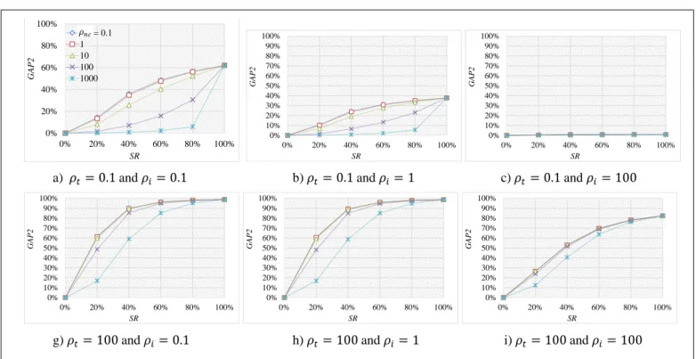
Fig. 4. Gap between 𝐸𝑇𝐶2and 𝐸𝑇𝐶1for some combinations of cost parameters
a) 𝜌𝑖= 0.1 b) 𝜌𝑖= 1 c) 𝜌𝑖= 10 -20% 0% 20% 40% 60% 80% 100% 0 1 10 100 SR GAP1 vs SR = 0 0.2 0.4 0.6 0.8 1 -40% -20% 0% 20% 40% 60% 80% 100% 0 1 10 100 SR GAP1 vs SR = 0 0.2 0.4 0.6 0.8 1 -200% -150% -100% -50% 0% 50% 100% 0 1 10 100 1000 SR GAP1 vs SR = 0 0.2 0.4 0.6 0.8 1
a) 𝜌𝑡= 0.1 and 𝜌𝑖= 0.1 b) 𝜌𝑡= 0.1 and 𝜌𝑖= 1 c) 𝜌𝑡= 0.1 and 𝜌𝑖= 100
g) 𝜌𝑡= 100 and 𝜌𝑖= 0.1 h) 𝜌𝑡= 100 and 𝜌𝑖= 1 i) 𝜌𝑡= 100 and 𝜌𝑖= 100 0% 20% 40% 60% 80% 100% 0% 20% 40% 60% 80% 100% GAP2 SR rnc = 0.1 1 10 100 1000 0% 10% 20% 30% 40% 50% 60% 70% 80% 90% 100% 0% 20% 40% 60% 80% 100% GAP2 SR 0% 10% 20% 30% 40% 50% 60% 70% 80% 90% 100% 0% 20% 40% 60% 80% 100% GAP2 SR 0% 10% 20% 30% 40% 50% 60% 70% 80% 90% 100% 0% 20% 40% 60% 80% 100% GAP2 SR 0% 10% 20% 30% 40% 50% 60% 70% 80% 90% 100% 0% 20% 40% 60% 80% 100% GAP2 SR 0% 10% 20% 30% 40% 50% 60% 70% 80% 90% 100% 0% 20% 40% 60% 80% 100% GAP2 SR
Figure 4 compares the performances of Policy 2 and Policy 3 by analyzing the gap between them. It proves that integrating quality control in supply and production planning reduces significantly the expected total cost whatever is the number of inspected products. We note that when inspection cost is much higher than the tardiness cost (Figure 4 c)), the policies are equivalent.
V. Conclusion
In this work, we are interested in supply and production planning under uncertainty of lead times and quality control. A model for supply planning of the production system and three quality control policies are analyzed. Experimental results highlights the economic advantage of integrating quality control planning at the early phase of supply planning optimization of production systems.
This exploratory study confirms the opportunity to extend this model by integrating maintenance activities and considering other kinds of production systems such as assembly systems where the finished products are assembled from several components.
Further, the second objective is to extend this model and different proposed technics to multi-period planning, in particular, calculate planned lead times when such a company deals with quality control, uncertainties of production and supply lead times.
References
[1] C. S. Tang, “The Impact of Uncertainty on a Production Line”, Management Science, 1990, 36(12), pp. 1518-1531. [2] D. C. Whybark and J. G. Williams, “Material Requirements planning under uncertainty”, Decision Science, 1976, 7(4), pp. 595-606.
[3] J. Weeks, “Optimizing planned lead times and delivery dates”, In 21st annual Conference Procceding, Americain Production and Inventory Control Society, 1984, pp. 177-188.
[4] C. A. Yano, “Setting Planned Leadtimes in Serial Production Systems with Tardiness Costs”, Management Science, 1987, 33(1), pp. 95-106.
[5] C. A. Yano, “Planned Lead-times for Serial Production Systems”, IIE Transactions, 1987, 19(3), pp. 300-307. [6] M. Elhafsi, “Optimal leadtimes planning in serial
production systems with earliness and tardiness costs”, IIE Transactions, 2002, 34, pp. 233-243.
[7] J. G. Kim, D. Sun, X. J. He and J. C. Hayya, “The (s,Q) inventory model with Erlang lead time and deterministic demand”, Naval Research Logistics, 2004, 51(6), pp.906-923.
[8] J. G. Kim, D. Chatfield, T. P. Harrison and J. C. Hayya, “Quantifying the bullwhip effect in a supply chain with stochastic lead time”, European Journal of Operational Research, 2006, 173(2), pp. 617-636.
[9] A. Dolgui, O. Ben-Ammar, F. Hnaien and M. A. Ould Louly, “A State of the Art on Supply Planning and Inventory Control under Lead Time Uncertainty”, Studies in Informatics and Control, 2013, 22(3), p. 255-268. [10] A. Dolgui and C. Prodhon, “Supply planning under
uncertainties in MRP environments: A state of the art”, Annual Reviews in Control, 2007, 31(2), pp. 269–279. [11] V. Guide and R. Srivastava, “A review of techniques for
buffering against uncertainty with MRP systems”, Production Planning & Control, 2000, 11(3), pp. 223-233. [12] M. A. Aloulou, A. Dolgui and M. Y. Kovalyov, “A bibliography of non-deterministic lotsizing models”, International Journal of Production Research, 2014, 52(8), pp.1-18.
[13] M. Díaz-Madroñero, J, Mula and D. Peidro, “A review of discrete-time optimization models for tactical production planning”, International Journal of Production Research, 2014, 52, pp. 5171-5205.
[14] M. Colledani and T. Tolio, “Impact of Quality Control on Production System Performance,” CIRP Ann. - Manuf. Technol., vol. 55, no. 1, pp. 453–456, Jan. 2006.
[15] M. J. Rosenblatt, and H. L. Lee, “Economic Production Cycles with Imperfect Production Processes”, IIE Transactions, 1986, 18(1), pp. 48-55.
[16] B. Bettayeb, N. Brahimi, and D. Lemoine, “Integrated Single Item Lot-Sizing and Quality Inspection Planning,” IFAC-PapersOnLine, vol. 49, no. 12, pp. 550–555, 2016. [17] O. Ben-Ammar, H. Marian, A. Dolgui, and D. Wu,
“Reducing the research space of possible order release dates for multi-level assembly systems under stochastic lead times”. Advances in Production Management Systems: Innovative and Knowledge-Based Production Management in a Global-Local World, Part III, Springer Series, 2014, vol. 440, pp. 368-374.