Computational measurements of stress fields from digital images

HAL Id: hal-01454432

https://hal.archives-ouvertes.fr/hal-01454432v2

HAL is a multi-disciplinary open access

archive for the deposit and dissemination of sci-entific research documents, whether they are pub-lished or not. The documents may come from teaching and research institutions in France or abroad, or from public or private research centers.

L’archive ouverte pluridisciplinaire HAL, est destinée au dépôt et à la diffusion de documents scientifiques de niveau recherche, publiés ou non, émanant des établissements d’enseignement et de recherche français ou étrangers, des laboratoires publics ou privés.

Computational measurements of stress fields from

digital images

Julien Réthoré

To cite this version:

Julien Réthoré. Computational measurements of stress fields from digital images. 2017. �hal-01454432v2�

Computational measurements of stress fields from digital images

J. R´ethor´e

Research Institute in Civil and Mechanical Engineering(GeM) Ecole Centrale de Nantes, Universit´e de Nantes

UMR 6183 CNRS, 1 rue de la No¨e, F-44 123 Nantes, France.

1

Introduction

Since the pioneering work of Lucas, Kanade and others [1], image registration or Digital Image Cor-relation (DIC) has been widely used and developed in many ways. For mechanical experimentalists, the purpose of DIC is to measure displacement fields by comparing digital images of the sample under two different loading states. Sub-set based techniques are the most popular ones (see for example [2]) because they are the techniques implemented in commercial softwares. One should also mention the non-parametric formulation proposed by [3] that allows for measuring a displacement field pixel-wise. Compared to the conventional experimental methodology for constitutive behaviour analysis, which consists in performing uni-axial homogeneous stress/strain tests, DIC has the major advantage to pro-vide for full displacement and strain fields. While this is useful to assess the quality of conventional tests, making good use of the rich data extracted from DIC measurements is still the purpose of many research works. One of the main issues is that the stress field in heterogeneous state configurations cannot be accessed without coupling measurements with numerical simulations.

Recently, Besnard et al.proposed a finite element (FE) formulation for DIC [4]. This considerably increases the potential of DIC as a strong coupling with FE simulations is established. For example, it is shown in [5] that both DIC and elastic balance of momentum can be solved at the same time. For the characterization of material constitutive relations, this opportunity to couple DIC measurements with FE simulations has been exploited to design robust identification techniques [6,7]. By identification we mean here estimating the parameters of a presupposed constitutive model. In some cases, making explicit a constitutive model and formalizing a constitutive law turns out to be extremely difficult. This is case for example for ductile tearing as the stress/strain and triaxiality levels occurring at tip crack cannot be reached in homogeneous stress/strain test configurations. At this point, the advantage of this framework (FE DIC combined with FE simulation) reveals also to be a weakness as it requires the constitutive relation to be explicit.

To circumvent the difficulty of formulating a constitutive equations, manifold learning or dimen-sionality reduction [8] are good candidates. The idea is to use databases of admissible material state (at least stress and strain) points to extract manifold and then to perform multi-dimensional inter-polation/regression for calculating internal forces in FE simulations. The data-driven computational mechanics framework recently proposed in [9] goes one step further. Instead of minimizing the energy under the constraint that the constitutive relation is satisfied, the authors propose in this work to minimize the distance between the computed material states and those given by a database under the constraint of equilibrium. These non-parametric approaches of the mechanics of materials have a great potential to circumvent the limitations of parametric approaches concerning the formulation of constitutive laws. However, if the database uses results from conventional experiments using ho-mogeneous stress/strain configurations, these promising methodologies would suffer from the same limitations concerning the lack of intense and/or complex loadings.

Full-field measurements could be used on heterogeneous states configuration to enrich material state databases with more complex configurations. However, as it has been mentioned above, the stress analysis of complex tests requires the coupling with FE simulations that need a constitutive model. This is disappointing to observe that these two advanced methods (one that extracts material data from experiments and the other that makes use of material state data to perform simulations) cannot help each other. At this point, one ends up with the following fundamental question:

Is it possible to measure stress fields ?

In general, it has not yet been possible. There exist some optical techniques like photo-elasticity, caustics, or more recently Diffraction Contrast Tomography (DCT), that allow to measure elastic stress fields but non-elastic stress evaluation is out of their scope. The aim of this paper is a proposition that may answer this question. It is not claimed that stress may become observable but we propose herein to formulate auxiliary problems involving DIC so that strain but also stress fields can be directly estimated with no assumption on the constitutive relation. Plus, a supplementary information is obtained that can be interpreted as an internal variable field that measures the distance between the actual local constitutive equation and linear elasticity according to a given but arbitrary elastic tensor.

The method will be referred to as Mechanical Image Correlation (MIC) as it allows to measure from digital images the local mechanical state of a material.

In the next Section, the principle of DIC is briefly explained. Then, the details of MIC are provided in Section3. In the last Section, some examples assessing the feasibility of the method and illustrating its potential are presented.

2

Digital Image Correlation (DIC)

The DIC framework used in the following is detailed in this section in a similar way as in [7]. This formalism is generic but convenient for the development presented in the next section.

2.1 Formulation

From two grey level images f and g of a given sample, DIC consists in a nonlinear minimization process that identifies the displacement field u that produces the advection of the local texture:

u = Arg Min X

p∈ROI

[f (xp) − g(xp+ u(xp))]2, (1)

where p is the index of a pixel within the Region Of Interest (ROI) over which the computation is performed and xp the co-ordinates of pixel p on the image frame. For solving this minimization

problem two main routes can be distinguished. A non-parametric route is proposed in [3]. In this approach, no assumption is made on the variation of displacement and the problem is solved pixel-wise using a staggered algorithm with relaxation and smoothing steps. The second route consists in a parametrization of the displacement as follows

u(x) = X

k∈N

ukNk(x). (2)

In this decomposition, N is the set of degrees of freedom (DOFs) uk, and Nkare the shape functions.

Different parametrization can be used. The particular case of crack tip fields required the use of Williams’ series as basis functions [10]. Other specific bases, like for 4-point bending test [11] or Brazilian test [12] can be used but for arbitrary displacement, finite element based [4, 13] or CAD based kinematics [14,15] are more appropriate.

From a first guess for the displacement, an iterative prodecure is run until convergence is reached. Assuming that the solution increment du is small enough, a first-order Taylor expansion of g(xp+

u(xp) + du(xp)) is used to linearize the functional. After some manipulations, we obtain that the

solution increment is calculated through:

[ ˜MDIC] {dU} = {˜bDIC}, (3)

with

[ ˜MDIC] = [N]T[∇G][∇G][N], (4)

and

{˜bDIC} = [N]T[∇G]{F − G}, (5)

∇ denoting spatial derivation. [N] is a matrix that collects the value of the basis functions at the pixels, [∇G] a diagonal matrix that collects the values of ∇g(xp+ u(xp)) and {F − G} a vector

containing the values of f (xp) − g(xp+ u(xp)). For the sake of clarity, indices indicating the iteration

number have been omitted. For a detailed description of the algorithm in a multiscale framework, and its implementation the interested reader may refer to R´ethor´e et al. [16]. To reduce computational cost, a modified algorithm is adopted: we substitute ∇G, which depends on the current solution vector, by ∇F. The modified system to solve thus becomes

with

[MDIC] = [N]T[∇F][∇F][N], (7)

and

{b_DIC} = [N]T[∇F]{F − G}. (8)

The advantage of such a modification is that MDIC and parts of bDIC can be computed once for all.

Note that when convergence is reached, ∇F equals ∇G. After a few iterations (2 or 3), the modified algorithm and the initial one reveal close to identical.

2.2 Condensation

At this point, it is interesting to draw the attention on the following assessment: for any parametriza-tion of the displacement field through Nk shape functions, DIC allows for estimating directly from

the images the corresponding DOFs uk. If Williams’ series are used as in [10], a direct access to stress

intensity factors is provided. An other interesting example is described in [6, 7]: the finite element displacement is considered as depending on the parameters of the constitutive law of the material. The DIC problem is then solved using not the full finite element parametrization but a combination of the finite element shape functions corresponding to the sensitivity of the displacement fields to the material parameters. In this context DIC provides for a measurement of the material parameters. In the next section (3), a parametrization of the displacement fields in terms of local stress is described. In other words, using appropriate combinations of finite element displacement degrees of freedom, one accesses to the local stress field which can thus be estimated by solving DIC with the proposed basis of nodal displacement vectors. The general solution algorithm for accessing the estimation of these generalized DOFs by DIC is derived below.

A general condensation method is proposed from a finite element parametrization of the displace-ment. In this case, Nkare finite element shape functions and uk nodal displacements. Let us consider

that the meaningful quantities are not the nodal displacements but linear combination of them. Given a linear condensation operator L, the nodal displacement U are then derived according to

{U} = [L] {Λ}. (9)

In this formalism, Λ collects the value of the generalized DOFs corresponding to the amplitude of the linear combination of nodal displacements defined by L. The DIC problem can be solved using this condensation with the following system

[MM IC] {dΛ} = {bM IC}, (10)

with

[MM IC] = [L]T [MDIC][L], {bM IC} = [L]T{bDIC}. (11)

3

Mechanical Image Correlation (MIC)

The approaches in [6,7], are parametric identification techniques: they allow for estimating experimen-tally the parameters of a constitutive law from digital images and load measurements corresponding to heterogeneous stress/strain states. These methods give access to a stress field compatible with the presumed constitutive law. As evidenced in the introduction, this is limiting in those cases when explicitly writing the constitutive equations is not possible. The purpose of this section is to propose a formulation giving access to local stress through the parametrization of an anelastic strain field.

3.1 Formulation

Let Co be an elastic operator. Then, an elastic solution uo, σσσo according to Co and balancing the

measured load Fo is computed using a standard finite element solver. The vector collecting the

constitutive law of the material, this reference solution uo, σσσo does not match the actual one u, σσσ. One

can define a gap in terms of displacement (kinematic gap) ¯u such that:

u = uo+ ¯u (12)

and a gap in terms of stress (static gap) ¯σσσ:

σσσ = σσσo+ ¯σσσ. (13)

The aim is now to find another route to define these gaps. The actual solution could then be retrieved from the reference solution and the gaps.

Because both σσσo and σσσ balance the external load, ¯σσσ is a self-balanced stress field. It admits the

following properties:

div¯σσσ = 0 over the ROI, ¯σσσn = 0 over the boundary of ROI, (14) However, there is a priori no straightforward relation between ¯σσσ and ¯u. Without loss of generality, one introduces an anelastic strain field εεεa such that

¯

σσσ = Co(¯εεε − εεεa) (15)

where ¯εεε is the symmetric gradient of the kinematic gap ¯u. Then using Equation (14), one obtains div(Co¯εεε) − div(Coεεεa) = 0 over the ROI, (Co(¯εεε − εεεa))n = 0 over the boundary of ROI (16)

It is thus clear that if εεεa is known then the gap from the reference solution to the actual one can be

retrieved and the latter can thus be computed. We will then proceed in two steps: first formulate auxiliary problems governing the anelastic strain εεεa, second find a parametrization of εεεa so that

the auxiliary problems can be solved and the actual solution recovered. Before these two steps are described, it is important to point that it is possible to separate εεεa fields in two contributions:

ε

εεa= εεεIa+ εεεIIa . (17)

Once the problem defined by Equation (16) is solved, a solution ¯u is obtained up to a rigid body motion. It is then possible to define the compatible part εεεI_a of εεεa as the symmetric gradient of ¯u:

εεεI_a= ¯εεε (18)

The remaining part εεεII_a = εεεa− εεεIais not compatible in general and it is not associated to any

displace-ment (¯uII = 0) as

div(CoεεεIIa ) = 0. (19)

The resulting self-balanced stress field is then written as ¯

σ

σσII = −CoεεεIIa . (20)

Conversely, εεεI_a induces a displacement ¯uI_a but no stress as εεεI_a= ¯εεε.

One ends up with two famillies of anelastic strain fields that are able to close the kinematic and static gap respectively. The following comments arise:

• εεεI

a being compatible, it is intrinsically related to a displacement (namely ¯u). If a set of basis

functions deriving from a set displacement functions is chosen for εεεI_a, they can be used as a basis for u by using Equation (12).

• the effect of εεεII

a is not observable (¯uII = 0).

3.2 Auxiliary problems

3.2.1 Type I As stated above, εεεI

afields can be used as a basis for ¯u and thus for u−uo. Then, using the condensation

of the DIC problem (Section2.2) as an auxiliary problem, the contribution of the εεεI_afields is obtained. Once a parametrization of εεεI_a is defined (see Section 3.3), a condensed DIC problem is used to close the kinematic gap ¯u.

3.2.2 Type II

Conversely, εεεII_a fields have no effect on ¯u, they are not observable and thus cannot be obtained from DIC. To retrieve uniqueness, one has to formulate an auxiliary problem constraining εεεII_a . It is proposed in the following that some information are given concerning the thermodynamics of the deformation process. For illustration purposes, three cases are investigated:

1. the material is homogeneous, its behaviour is linear and there is no dissipation: in this case there exists C such that σσσ = Cεεε. Assuming that εεε is known (from DIC), then the governing equation for εεεII_a is

CoεεεIIa = σσσo− Cεεε (21)

2. the material is not homogeneous but it is isotropic (Co is taken isotropic as well), its behaviour

is linear and there is no dissipation. In this case, one can define a constrast field φ such that σσσ = φCoεεε. Assuming that εεε is known (from DIC), then the governing equation for εεεIIa is

CoεεεIIa = σσσo− φCoεεε (22)

3. the material is homogeneous, isotropic and elastoplastic with isotropic. Its elastic behaviour is defined by Co which is assumed to be isotropic. Then assuming that the plastic flow occurs

following the normality rule, the principle of maximum dissipation applies. The problem is rephrased incrementally and an increment ∆εεεII_a of anelastic strain between two time instants is searched to maximize

(σσσo− Co(εεεIIa + ∆εεεIIa )) : (∆εεεIa+ ∆εεεIIa ) (23)

Searching for the stationarity of the dissipation as defined above leads to a linear problem in ∆εεεII_a .

Obviously, these auxiliary problems cannot be solved point wise. One first needs a parametrization of εεεII_a and then to solve these problems in a least-squares sense. The former points is the purpose of the next Section.

3.3 Parametrization

Using usual finite element settings, a 2D mesh of Ne simplex elements is considered. From this mesh,

a strain basis of 3 × Ne components is considered. The 3 × Ne finite element internal force vectors Fint

(2 × N components) with Co as constitutive operator is elaborated. A singular value decomposition of

these vectors is performed to extract their linear combination giving rise to non-zero internal forces. Up to NI = 2 × N − 3 combinations (denoted as Ea) can be obtained. If Ko denotes the finite

element elastic stiffness matrix with Co as constitutive operator then, NI displacement solutions V

are obtained from the resolution of the linear systems defined as

[Ko] {V} = [Fint]{Ea} (24)

The stress fields

Σ = Co(∇SV − Ea) (25)

are computed and type I and type II fields are coputed according to their definition (Equations (17), (18). The following parametrizations are introduced:

I ¯UI = V, EI_a= ∇SV, ΣI= 0,

II EII_a = Ea− ∇SV, ¯UII = 0, ΣII = Σ.

Note that the number of terms in each of these parametrizations can be ajusted independently, namely NI and NII.

For solving the auxiliary problem I (Section3.2.1), one needs a parametrization of the displacement u. The first component of this parametrization is Uo. This displacement vector is obtained from a FE

elastic simulation using Co as the elastic tensor and a prescribed displacement measured by DIC along

the boundary of the ROI where non-zero stress conditions apply. The amplitude of this displacement is adjusted so that the resulting forces Fo match the experimental data. Note that because Co may

not be the actual constitutive operator, after adjustment of Fo, the displacement along the boundary

of the ROI does not match the measured displacement anymore.

The next terms of the displacement parametrization are obtained from the anelastic fields, namely UI. This parametrization does not contain rigid body motions (two translations and one rotation in 2D) that are considered through additional basis vectors in UR. These bases are then concatenated

as ¯U = [UIUR] for describing ¯u.

3.4 Resolution

3.4.1 Type I

A parametrization of the anelastic strain field is proposed above. Concerning the displacement, the amplitude of one of the basis functions is known a priori to ensures that the external force resulting from the measured stress matches the measured force. The deformed image g is thus advected by uo + ¯u and the DIC problem solved with respect to the parameter involved in the parametrization

[ ¯UI] only. Following Section 2.2, the DIC problem is solved with a condensation operator L equal to ¯

UI_.

Using the proposed methodology, DIC provides for the NI amplitudes of [ ¯UI] components, let us

say ¯ΛI. This of course gives a direct access to the measured displacement and total strain field. In a post-processing step, anelastic strain field εεεI_a is derived from EI_a and the corresponding components of

¯ ΛI.

3.4.2 Type II

For computing εεεII_a , one of the auxiliary problems presented in Section 3.2.2 is solved. All these problems are linear and once the parametrization EII_a is adopted, they recast as

[P ][EII_a I]{ ¯ΛIIA} = {Q} (26) where P is a Ne × NII matrix collecting the linear contraints of the auxiliary problem II in each

element of the mesh, Q collects Nevalues for the constraints. The identity matrix I and the additional

parameters vector A account for the contribution of additional quantities like C for case 1 or unknowns defining the variation of φ for case 2. This linear system of equations is solved in a least-square sense providing for the NII amplitudes ¯ΛII of the parametrization for εεεIIa . ¯σσσ is then reconstructed using

ΣII and the actual stress field is reconstructed. Also the additional parameters are identified like the actual elastic tensor C for case 1 or the contrast field φ for case 2.

Note that, while thermodynamic assumptions considered in the auxiliary problems constrain the type of constitutive law satisfied by the actual fields, the decomposition adopted herein is completely generic. An other important point is that any combination of components of the proposed basis satisfies the local balance of momentum.

4

Examples

To illustrate the capability of the proposed method to measure stress, strain and anelastic strain fields from digital images, synthetic data are generated. A finite element simulation is run and the result from this simulation is used to generate a set of deformed images given a reference speckle pattern. Three examples illustrating the three auxiliary problems formulated in the previous are proposed.

4.1 Anisotropic linear elasticity

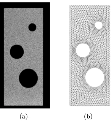
In this example, the model consists in a rectangular domain of 1800 × 3800 pixels with three holes of different diameter. The reference image is shown by Figure 1(a). In the FE simulation used for

generating the synthetic data, the displacement along the bottom edge is clamped while along the top edge, the vertical displacement is set to 0, 30 and 30 pixels. The horizontal displacement is prescribed to 30, 0 and 30 pixels. In this numerical simulation the material is assigned a linear orthotropic behaviour Ci defined as Ci =   5.56 1.39 0.00 1.39 55.56 0.00 0.00 0.00 4.16   x,y GPa (27)

in the x, y co-ordinate system of the reference image. The synthetic images are generated using a very fine mesh, 4 times finer than that used in the following for MIC and depicted in Figure1(b). In this mesh, the element size is 60 pixels far from the holes and 40 pixels in the vicinity of the holes. This mesh contains 1539 nodes and 2808 triangular elements with linear interpolation.

For the MIC analysis, Co is set as an isotropic elastic tensor having its Young’s modulus and

Poisson’s ratio set to 5 GPa and 0.2 respectively. The number of εεεI_afunctions is set as high as possible (2×1539−3) whereas εεεII

a is described with 500 modes. The displacement fields for the three load steps

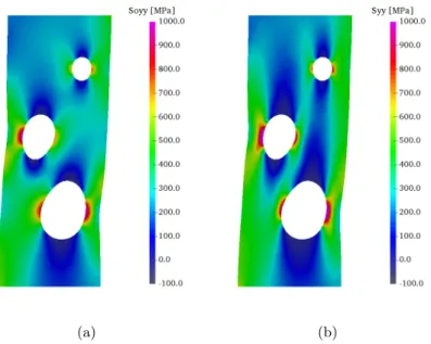
are presented in Figure2. For illustration purposes, the reference stress field σσσo and the reconstructed

stress field σσσ are plotted in Figure 3 for the last load step. It is worth noting that they differ in the vicinity of the holes while they are similar close to the bottom and top edges as their vertical component are the main contribution to the external load which both of them balance. To assess the reliability of the stress estimate, it is compared on Figure4 to a stress field obtained by applying the actual elastic tensor Ci to the measured strain field. Indeed, due to discretization effects, it is not

possible to compared the reconstructed stress to the numerical simulation used for image generation. The error in the stress field is plotted in Figure 4 with different colorscale. On Figure 4(b), the colorscale has the same amplitude as for representing σσσ itself whereas this amplitude is reduced by a factor of 10 in Figure4(a). This allows one to appreciate the robustness of the estimation. Indeed, the average difference between the estimated stress field and its theoretical value is about 9 Mpa and the standard deviation of this difference is about 67 Mpa. Compared to a maximum stress value higher than 1000 Mpa, it is stated that the uncertainty is around 5%. Also, the auxiliary problem provides an estimate of the elastic tensor. The following values are obtained:

C =   7.4 1.60 0.05 1.60 51.75 0.65 0.05 0.65 4.60   x,y GPa. (28)

The accuracy is again around 5%. To further illustrate the capability of the proposed approach, a three dimensional plot of the vertical stress as a function of the measured vertical and horizontal strain is proposed in Figure5. One might notice that the region of the stress/strain domain with low signal (low stress and low vertical strain) concentrates the points with highest error. There is also high error points for high stress corresponding to the hole boundary where the strain measurement is less reliable. However, it is shown through this example that MIC provides not only for displacement and strain fields but also for reliable stress field estimates as well as the full elastic tensor from one single test configuration.

4.2 Heterogeneous isotropic elasticity

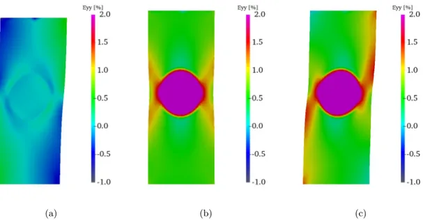
In this second example, the same rectangular plate as before is considered. However, instead of having holes, an soft circular inclusion (the contrast is set to 0.1) is included in the center of the plate (see Figure6(a)). The same loading scenario as in the previous example is modeled. While the mesh used for the simulation generating the images explicitly describes the inclusion, the mesh for MIC and the images are built without considering the inclusion (see Figures6(b)and6(c)). The MIC mesh contains 1969 nodes for 3773 elements of around 50 pixels.

For the MIC analysis, Co is set as an isotropic elastic tensor having its Young’s modulus and

Poisson’s ratio set to 5 GPa and 0.2 respectively. This is the elastic model used outside the inclusion for generating the images. The number of modes for εεεI_a is set to 500 while for εεεII_a it is set to 100 modes. The variation of the contrast field φ is described with the finite element linear shape function

of the mesh in Figure6(c). It is worth noting that the material discontinuity considered for generating the images cannot be captured exactly. A smoothing of the identified contrast field is expected across the inclusion boundary.

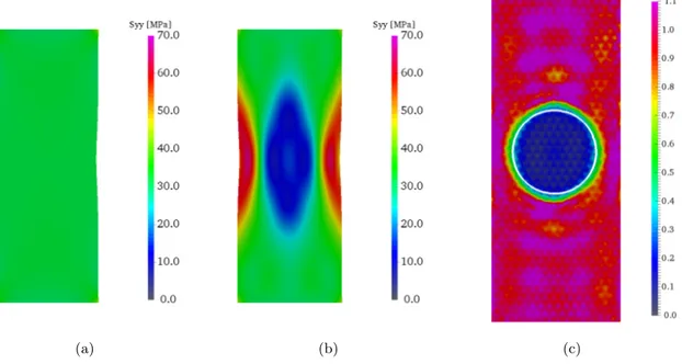
On Figure 7, the vertical component of the strain tensor for the three load steps are presented. One clearly observes the strain concentration in the matrix around the hole and very high but quasi homogeneous strain within the soft inclusion. Using the auxiliary problem 2 in Section 3.2.2, εεεII_a is obtained for reconstructing the stress field from the reference solution. As the material is homogeneous in the reference problem, for the second load step that corresponds to uniaxial tension, σσσo is almost

homogeneous in the sample (see Figure8(a)). The gap to be compensated by ¯σσσ to recover the actual stress is large and heterogeneous. However, in Figure8(b), the expected stress concentration around the hole is recovered. The emphasis is here on the ability of the approach to identify material property field. For this purpose, the identified contrast field φ is plotted on Figure8(c). The white circle in this Figure defines the actual boundary of the inclusion as considered in the simulation used for generating the images. Although the mesh used to perform MIC is uniform, a very good agreement is obtained on the geometry of the inclusion. Further, the stiffness contrast between the inclusion and the matrix is captured. The average error on the contrast over the whole sample is 0.02 while the standard deviation of the error is 0.13.

4.3 Elasto-plasticity

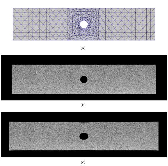
A rectangular sample of 100 × 20mm2 with a hole of diameter 5 mm is considered. It is assigned an elasto-plastic behaviour with linear isotropic hardening. The Young’s modulus is 168 GPa, the initial yield stress 284 MPa and the hardening coefficient 1.48 GPa. The Poisson’s ratio is 0.25. The numerical simulation is run with a mesh similar to that shown in Figure9(a) but with one additional subdivision. A 2D plane stress formulaton is used. The reference image is depicted in Figure 9(b)

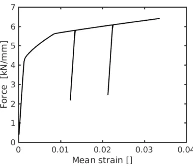
and last deformed image in Figure 9(c). The size of the images is 5120×1400 pixels, corresponding to a physical pixel size of 22.2 µm. The speckle pattern for the initial image is a real one taken from an image of a real sample. The load history applied in the simulation is illustrated in Figure 10. 200 steps are performed. Two unloading stages are considered at step 40 and 120.

The MIC analysis is run using 500 type I modes and 300 type II modes. The elastic tensor Co

is assigned the same value as the elastic tensor for the numerical simulation used to generate the images. In the DIC analysis, the displacement estimation along the boundary of the finite element mesh are usually less robust than in the bulk. To avoid that this lower robustness affects the result of the MIC analysis where the DIC displacement is used as boundary conditions for computing the admissible elastic solution uo, one layer of elements is removed at both ends of the mesh. The DIC

displacement used as boundary conditions is thus picked up from nodes in the bulk of the DIC mesh. The displacement fields measured by DIC and MIC using the mesh in Figure9(a)for the last loading step are depicted in Figure 11. The scatter between the two displacements is difficult to observe by the naked eyes. For assessing the accuracy of the displacement field obtained by MIC, the correlation error map are plotted for the two analyses in Figure 12. These two error maps are again difficult to distinguish what confirms that the MIC displacement leads to a registration of the images of the same accuracy as the DIC analysis. To further assess this point, the average correlation error for DIC and MIC is plotted as a function of the steps in Figure 13. The error level is slightly higher for MIC, what is expected because only 500 modes are used to measure the displacement instead of 2 × N . The search of the optimal solution in terms of grey level conservation is thus more constraint and the minimum error level reached with the reduced parametrization is higher. These results ensure that the displacement parametrization adopted for MIC leads to measured fields globally as accurate as thoses obtained for a DIC analysis.

MIC also provides for the estimation of meaningful mechanical fields. First the evolution of the stress component in the loading direction is provided in Figure 14. The decrease in stress during unloading is well captured, as well as its progressive increase during the loading stages. In Figure15, the norm of the anelastic strain ¯εεεa is plotted for the same steps as the stress in Figure 14. It is

observed, as expected for an elasto-plastic material for which εεεacorresponds to the plastic strain, that

contribution of the out-of-plane component which has been derived using plastic incompressibility. The latter is plotted for the last step in Figure 16. Expected results like shrinkage at the pole of the hole are retrieved.

To further illustrate the capability of MIC to measure stress fields, an analysis of the entire set of measured material states is provided in Figure 17. This set consists in more than 600 000 points in the space defined by the components of stress, strain and anelastic strain tensors. For visualization purposes, ones needs to reduce the dimensionality of this database. Because it is assumed that von Mises plasticity holds, the von Mises stress is computed as well as the deviatoric part of the elastic strain and the norm of the anelastic strain. In Figure 17(a), the evolution of the von Mises stress is plotted as a function of the norm of the plastic strain for a few points. The typical loading unloading scenario of elasto-plasticity is captured. In Figure 17(b), von Mises stress is plotted as a function of the deviatoric part of the elastic strain and the norm of the plastic strain. The shape of the domain of admissible material states agrees well with the one considered in the numerical simulations to generate the images.

5

Conclusion

A methodology is proposed to build, in a general case, a parametric description of the displacement and stress fields based on an anelastic strain field. DIC is used to obtained part of the parameters of this description whereas the other part is obtain thanks to thermodynamic assumptions on the deformation proccess leading to an auxiliary problem. The resolution of this problem allows for computing the stress field. With no assumption on the constitutive relation, the method allows for measuring displacement, strain but also stress fields. Further, an anelastic strain field measuring the distance between the actual local constitutive behaviour and elasticity according to a given but arbitrary elastic tensor is obtained. The ability of the method to measure stress fields in different situations is illustrated. The raw data extracted from the measurement are admissible material states in a space of dimension 9 for 2D problems.

6

Acknowledgments

The support of R´egion Pays de la Loire and Nantes M´etropole through grant Connect Talent IDS is gratefully acknowledged.

References

[1] Lucas BD, Kanade T, et al.. An iterative image registration technique with an application to stereo vision. IJCAI, vol. 81, 1981; 674–679.

[2] Sutton M, Cheng M, Peters W, Chao Y, McNeill S. Application of an optimized digital im-age correlation method to planar deformation analysis. Imim-age Vision Computing august 1986; 4(3):143–150.

[3] Vercauteren T, Pennec X, Perchant A, Ayache N. Diffeomorphic demons: Efficient non-parametric image registration. NeuroImage 2009; 45(1):S61–S72.

[4] Besnard G, Hild F, Roux S. ‘finite-element’ displacement fields analysis from digital images: Application to portevin-le chˆatelier bands. Experimental Mechanics 2006; 46(6):789–803.

[5] R´ethor´e J, Hild F, Roux S. An extended and integrated digital image correlation technique applied to the analysis of fractured samples. European Journal of Computational Mechanics 2009; 18:285– 306.

[6] Leclerc H, Perie J, Roux S, Hild F. Computer Vision/Computer Graphics CollaborationTech-niques, chap. Integrated Digital Image Correlation for the Identification of Mechanical Properties. Springer: Berlin, 2009.

[7] R´ethor´e J. A fully integrated noise robust strategy for the identification of constitutive laws from digital images. International Journal for Numerical Methods in Engineering 2010; 84:631–660, doi:10.1002/nme.2908.

[8] van der Maaten L, Postam E, van den Herik J. Dimensionality reduction: A comparative re-view. Technical Report, Tilburg, Netherlands: Tilburg Centre for Creative Computing, Tilburg University, Technical Report: 2009-005 2009.

[9] Kirchdoerfer T, Ortiz M. Data-driven computational mechanics. Computer Methods in Applied Mechanics and Engineering 2016; 304:81–101.

[10] Roux S, Hild F. Stress intensity factor measurement from digital image correlation: post-processing and integrated approaches. International Journal of Fracture 2006; 140(1-4):141–157. [11] Leplay P, R´ethor´e J, Meille S, Baietto M. Damage law identification of a quasi brittle ceramic from a bending test using digital image correlation. Journal of the European Ceramic Society 2010; 30(13):2715–2725.

[12] Hild F, Roux S. Digital image correlation: from displacement measurement to identification of elastic properties–a review. Strain 2006; 42(2):69–80.

[13] R´ethor´e J, Hild F, Roux S. Extended digital image correlation with crack shape optimization. International Journal for Numerical Methods in Engineering 2008; 73(2):248–272, doi:10.1002/ nme.2070.

[14] Elguedj T, R´ethor´e J, Buteri A. Isogeometric analysis for strain field measurements. Computer Methods in Applied Mechanics and Engineering 2011; 200(1-4):40–56.

[15] R´ethor´e J, Elguedj T, Simon P, Coret M. On the use of nurbs functions for displacement deriva-tives measurement by digital image correlation. Experimental Mechanics 2009; 50(7):1099–1116, doi:10.1007/s11340-009-9304-z.

[16] R´ethor´e J, Hild F, Roux S. Shear-band capturing using a multiscale extended digital image correlation technique. Computer Methods in Applied Mechanics and Engineering 2007; 196(49-52):5016–5030, doi:10.1016/j.cma.2007.06.019.

7

Figures

(a) (b)

(a) (b) (c)

Figure 2: Displacement magnitude in pixel for the three load steps in the case of anisotropic elasticity (amplification factor 5).

(a) (b)

Figure 3: Reference stress and actual stress field estimate (vertical component) in the case of anisotropic elasticity (last load step, amplification factor 5).

(a) (b)

Figure 4: Error assessement on the vertical component of the estimated stress in the case of anisotropic elasticity (last load step, amplification factor 5).

Figure 5: Vertical stress as a function of the measured vertical and horizontal strain in the case of anisotropic elasticity. The dots correspond to measurements while the plane is the prescribed elastic tensor. The color of the dots defines the distance to the plane.

(a) (b) (c)

Figure 6: Test configuration, reference image and mesh for MIC analysis in the case of heterogeneous elasticity.

(a) (b) (c)

Figure 7: Vertical strain field for the three load steps in the case of heterogeneous elasticity (amplifi-cation factor 5).

(a) (b) (c)

Figure 8: Reference stress and actual stress field estimate (vertical component) and identified contrast field (second step, amplification factor 5).

(a)

(b)

(c)

Figure 9: Finite element mesh for the MIC analysis. Initial and last images generated from the FE simulation.

(a)

(b)

Figure 11: Displacement (in pixel) in the loading direction at the last step for (a) a DIC analysis and (b) a MIC analysis.

(a)

(b)

Figure 12: Correlation error map in grey level at the last step for (a) a DIC analysis and (b) a MIC analysis.

(a)

(b)

(c)

(d)

(e)

Figure 14: Evolution of the stress component in the axial direction in MPa: (a) just before the first unloading, (b) at the first unloading, (c) just before the second unloading, (d) at the second unloading and (e) at the last step.

(a)

(b)

(c)

(d)

(e)

Figure 15: Evolution of the anelastic strain norm: (a) just before the first unloading, (b) at the first unloading, (c) just before the second unloading, (d) at the second unloading and (e) at the last step.

(a) (b)