HAL Id: tel-01420419
https://pastel.archives-ouvertes.fr/tel-01420419
Submitted on 20 Dec 2016HAL is a multi-disciplinary open access
archive for the deposit and dissemination of sci-entific research documents, whether they are pub-lished or not. The documents may come from teaching and research institutions in France or abroad, or from public or private research centers.
L’archive ouverte pluridisciplinaire HAL, est destinée au dépôt et à la diffusion de documents scientifiques de niveau recherche, publiés ou non, émanant des établissements d’enseignement et de recherche français ou étrangers, des laboratoires publics ou privés.
Usman Niaz
To cite this version:
Usman Niaz. Cutting the visual world into bigger slices for improved video concept detection. Image Processing [eess.IV]. Télécom ParisTech, 2014. English. �NNT : 2014ENST0040�. �tel-01420419�
EDITE - ED 130
Doctorat ParisTech
T H È S E
pour obtenir le grade de docteur délivré par
TELECOM ParisTech
Spécialité « Signal et Images »
présentée et soutenue publiquement par
Usman Farrokh NIAZ
le 08 juillet 2014
Cutting the Visual World into Bigger Slices for Improved Video
Concept Detection
Amélioration de la détection des concepts dans les vidéos par de plus grandes tranches du Monde Visuel
Directeur de thèse :Bernard Mérialdo
Jury
M. Philippe-Henri Gosselin,Professeur, INRIA Rapporteur
M. Georges Quénot,Directeur de recherche CNRS, LIG Rapporteur
M. Georges Linares,Professeur, LIA Examinateur
M. François Brémond,Professeur, INRIA Examinateur
M. Bernard Mérialdo,Professeur, EURECOM Encadrant
TELECOM ParisTech
Visual material comprising images and videos that surrounds us is growing ever so rapidly over the internet and in our personal collections. This necessitates automatic understanding of the visual content to conceive intelligent methods for correctly indexing, searching and retrieving images and videos. We have entered an age where the reliance of humanity on computing has never been felt so strongly before. However we still are not able to make our machines see and understand the world around us like we humans do. Initial successes in Computer Vision after the conception of the field some 50 years ago encouraged the then scientist to predict the successful resolution of the problem of automatic understanding of visual material with in some years. 5 decades on and our computers still achieve partial success in truly detecting the content depicted in an images, let alone a video.
The difficult task of automatic indexing and retrieval of videos based on their content is abundantly addressed by academic and industrial exploration. Decades of research on text based automatic retrieval and then content based methods to index videos has led to the development of ingenious systems. These complex systems mainly utilize image analysis and statistical learning tools and more or less comprise of several intricate steps to make the machine able to recognize the content. However unlike text based search, automatic understanding of the video content is far from solved with our machines today using the current methods. A vast amount of information is extracted from videos some of which is used efficiently and cleverly to achieve the target being mindful to the scalability and complexity of the system.
Understanding the importance of content based indexing and retrieval and after doing extensive research of the state of the art in the field we feel that the automatic system can be improved in many ways. We predominately target the information that is not used when building such a system, whilst its already there. This thesis aims at improving the automatic detection of concepts in the internet videos by exploring all the available information and putting the most beneficial out of it to good use. We look at it in the sense of cutting thicker slices from the vast world of visual information to build our categorization system.
Our contributions target various levels of the concept detection system in videos and propose methods to improve the global performance of the inter disciplinary system. The standard system extracts low level information from the videos and givens a decision about the presence of an entity in the video frame after a series of computing steps. Our con-tributions start with improving the video representation model employing some existing information from the Visual World. We then devise methods to incorporate knowledge from similar and dissimilar entities to build improved recognition models. Lastly we contrive cer-tain semi-supervised learning methods to get the best of the substantial amount of unlabeled data.
During the latter half of 2010, owing to the unfolding of a series of unfortunate events, I had become quite clueless and disheartened. Fortunately enough, Professor Bernard M´erialdo hired me to do PhD research under his supervision, I was rescued. With computer vision being my research passion, finding a PhD thesis in the topic with an excellent professor was like a dream come true. I would like to start these acknowledgments by expressing my profound gratitude to professor M´erialdo for his continuous support, his careful guidance, his positive attitude, his advices, his patience and for some of the morale boosting sessions we had.
I would also like to thank Professor Lionel Pr´evost (UPMC, UAG) as he was always a source of inspiration for me for the very short period of time we worked together and played a very important role in getting me the PhD position at Eurecom.
I felt at home in Eurecom right from the start. With a wonderful mix of people from beautiful and fabulous countries, having amazing and friendly personalities I felt welcomed since my first day. In the old campus we were five in a big room, including a Turkish, a Tunisian, an Italian and then a Cameroonian, an Argentinean and me, a Pakistani. The seniors were always ready to help and offered helpful advices. Then there was always someone bringing special treats from their respective countries, to share with everyone. Birthdays, pot de th`eses and ’MMtalks’ were another medium of getting everyone together. I wish to thank Claudiu and Miriam for their guidance and specially Miriam for her reassurances of, ’don’t worry, Its going to be fine’. I can never forget the discussions I used to have with Claudiu about ’where we stand’ (and where should we stand). I would like to thank Simon, Hajer, Neslihan, Huda, Federico, Gislain, Ravi, Giovanni, Leela, Christelle, Jos´e and of course my Pakistani friends in Eurecom Sabir and Imran. The role of all the secretaries, HR and the guys at IT help-desk, with whom we PhD students had frequent interaction, can not go unacknowledged. It is their excellent service, helpful attitude and proper guidance that makes them stand apart, making your life wonderful at Eurecom. Finally, life bound to be wonderful if you are working and living in one of the most enviable places in the world, specially Europe, the French Riviera. In the south of France enjoying around 300 days of sunlight a year gives one enough time and opportunities to relax, stay healthy and come to work with a fresh mind.
During my PhD at Eurecom I worked on the ANR’s SUMACC project in collaboration with other expert partners. During the project meetings I had the chance to meet bril-liant people and learn from them including professor Georges, Christophe, Claude, Cl´ement, Mohamed and Richard.
Words aren’t enough to encompass the immense gratitude i owe to my wonderful parents. All I can do is thank them for always treating my worries as their top priorities. They’ve not only been my mentors but my friends and have always been a source of motivation,
inspiration and guidance for me. I attribute much of the success in my life to my mother’s prayers and her constant guidance. Not a single conversation with her ever ends without me learning something new, something useful. My father on the other hand see’s things on the lighter side and encourages us to do the same as well. I believe it is the perfect parental combination one could hope for and it has worked perfectly for me (and my siblings) even though I was away from home for a long time, completing my higher studies.
And finally I cannot conclude without thanking the most important person who was there with me during a good part of my PhD, my wife Bushra. Since I’ve gotten to know her she’s been a constant support in every aspect of my life. She’s been with me through all the ups and downs, that come your way specially in pursuit of a PhD, far away from home, supporting me and proudly standing by my side, and I know that she’ll always be there for me. She has always believed in me and cherished me with her amazing and supportive words and her beautiful smile.
Abstract i
Acknowledgements ii
List of Figures ix
List of Tables xi
1 Introduction 1
1.1 Video Concept Detection (Semantic Indexing) . . . 2
1.2 Video Concept Detection Pipeline . . . 3
1.3 Motivation . . . 8
1.3.1 Making the Slice Bigger . . . 9
1.4 Our Contributions . . . 10
2 State of the Art 13 2.1 Feature Extraction . . . 14
2.1.1 Global Features. . . 14
2.1.2 Local Features . . . 15
2.2 Feature Coding and Pooling . . . 16
2.3 Classification . . . 18
2.3.1 Generative Models . . . 18
2.3.2 Discriminative Models . . . 19
2.4 Fusion . . . 19
2.4.1 Feature Level Fusion . . . 20
2.4.2 Decision Level Fusion . . . 20
2.5 Evaluation. . . 21
3 Enhancing Video Representation 23 3.1 Visual Dictionary Construction/BOW Model . . . 24
3.1.1 The Dictionary Size . . . 25
3.1.2 Loss of Contextual Information . . . 26
3.1.3 Loss of Descriptor Specific Information. . . 26
3.1.4 Some Relevant Works . . . 26
3.2 Entropy based Supervised Merging . . . 28
3.2.1 Supervised Clustering Based on Entropy Minimization . . . 30
3.2.1.1 Concept Distribution Entropy Minimization . . . 30 v
3.2.1.2 Concept Dependent Entropy Minimization . . . 32
3.2.1.3 Average Concept Entropy Minimization . . . 33
3.2.1.4 Relaxing Constraints . . . 33
3.2.2 Experiments . . . 34
3.2.2.1 Supervised Clustering Results . . . 34
3.2.2.2 Alternative Mappings . . . 35
3.2.2.3 Small and Informative vs Large Dictionaries . . . 37
3.3 Intra-BOW Statistics . . . 39
3.3.1 Difference BOW . . . 40
3.3.1.1 Weighted DBOW . . . 42
3.3.2 Experiments . . . 43
3.3.2.1 Experimental Setup . . . 43
3.3.2.2 Hamming Embedding Similarity Feature . . . 44
3.3.2.3 Results . . . 45
3.4 Conclusions . . . 47
4 Leveraging from Multi-label Data 49 4.1 Learning from Multi-label Datasets and State of the Art . . . 50
4.1.1 Multi-label Classification . . . 51
4.1.2 Knowledge Transfer and Semantic Sharing. . . 53
4.1.2.1 Visual Attributes . . . 54
4.1.2.2 Hashing and Binary Codes . . . 55
4.1.2.3 Repetetive Codes . . . 56
4.2 Group SVM . . . 59
4.2.1 Group Based Classification . . . 60
4.2.1.1 Clever Grouping . . . 61
4.2.2 Experiments and Results . . . 64
4.2.2.1 Experimental Setup . . . 64
4.2.2.2 Results . . . 65
4.3 Label Clustering and Repetitive Codes . . . 69
4.3.1 Proposal. . . 70
4.3.1.1 Code Generation by Clustering . . . 71
4.3.1.2 Decoding for Ranked Predictions . . . 74
4.3.1.3 Ensemble of ECOCs . . . 75
4.3.2 Results and Experiments . . . 75
4.3.2.1 Datasets and Setup . . . 75
4.3.2.2 Results . . . 76
4.4 Label Trees and Repetitive Codes. . . 83
4.4.1 Proposed Approach . . . 84
4.4.1.1 Tree Construction . . . 84
4.4.1.2 Ternary Codes and Error Correction . . . 86
4.4.1.3 Ensemble of Trees, Forest . . . 88
4.4.2 Results and Experiments . . . 88
4.4.2.1 Datasets and Setup . . . 88
4.4.2.2 Results . . . 88
5 Leveraging from Unlabeled Data 95
5.1 Semi-supervised Learning for Retrieval . . . 95
5.1.1 Cotraining for Video Analysis: A review . . . 97
5.2 Selective Multi Co-training . . . 98
5.2.1 Proposed Approach . . . 98
5.2.1.1 Selecting the Most Complementary View . . . 99
5.2.1.2 Selection Methods . . . 99
5.2.2 Results and Experiments . . . 103
5.2.2.1 Experimental Setup . . . 103
5.2.2.2 Results . . . 103
5.3 Conclusions . . . 107
5.3.1 Restrained Multi-view Learning. . . 107
6 Conclusions 111 6.1 Key Contributions . . . 111
6.2 Promising Directions . . . 113
6.2.1 Immediate Future Work . . . 113
6.2.2 General Perspectives . . . 114
A Our Contributions 117 B Am´elioration de la d´etection des concepts dans les vid´eos par de plus grandes tranches du Monde Visuel 119 B.1 R´esum´e . . . 119
B.2 Introduction. . . 120
B.2.1 La d´etection des concepts dans les vid´eos, Indexation S´emantique. . . 121
B.2.2 Le Pipeline du d´etection . . . 123
B.2.3 Motivation . . . 128
B.2.4 Elargissant la tranche . . . 129
B.2.5 Nos Contributions . . . 130
B.3 Nos Contributions . . . 131
B.3.1 Pour une meilleure repr´esentation de la vid´eo . . . 131
B.3.2 S’appuyant sur des donn´ees multi-´etiquet´es . . . 132
B.3.3 Classification semi supervis´e. . . 133
B.4 Conclusions et Perspectives d’Avenirs . . . 135
B.4.1 Les contributions cl´es . . . 135
B.4.2 Des directions prometteuses . . . 137
B.4.2.1 Les perspectives d’avenir imm´ediat. . . 137
B.4.2.2 Les perspectives d’avenir g´en´erale . . . 138
1.1 Video Concept Detection . . . 2
1.2 Video Concept Detection Pipeline. . . 4
1.3 Global and local feature extraction example.. . . 5
1.4 Coding and pooling to generate the summarized feature for an image. . . 6
1.5 (a) A discriminative classifier separating positive and negative examples. (b) A generative classifier adapted to the positive concept examples. . . 7
1.6 Classifier fusion at the decision level. . . 8
1.7 The Visual World with numberous images, feaures and classifiers. . . 10
3.1 Visual Dictionary construction and histogram vector generation . . . 25
3.2 Related keypoints in neighboring cells: label information from images is used to merge the Voronoi cells . . . 29
3.3 Unrelated keypoints in a clustering cell: label information from images is used to split the Voronoi cell . . . 30
3.4 Supervised merging of visual words . . . 31
3.5 Related keypoints in neighboring cells: label information from images is used to merge the Voronoi cells . . . 32
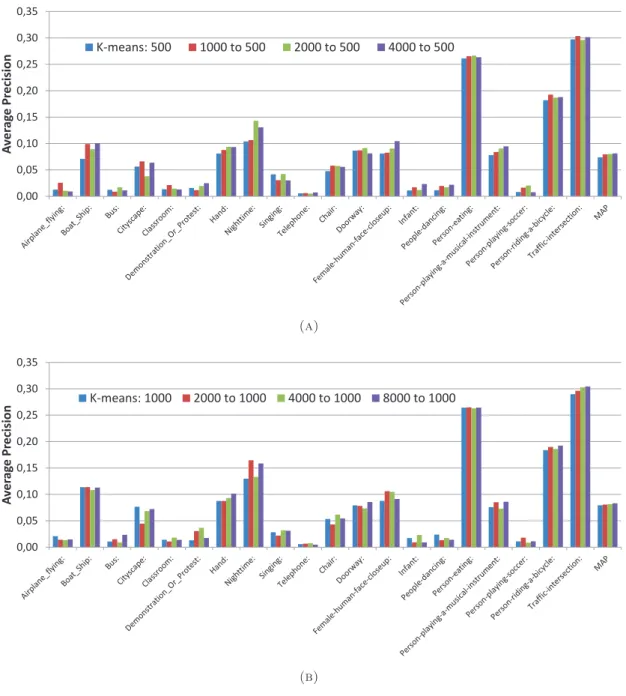
3.6 Supervised clustering scores for 20 concepts using the first (best) entropy minimization criterion for (a) 500 and (b) 1000 visual words dictionaries . . . 36
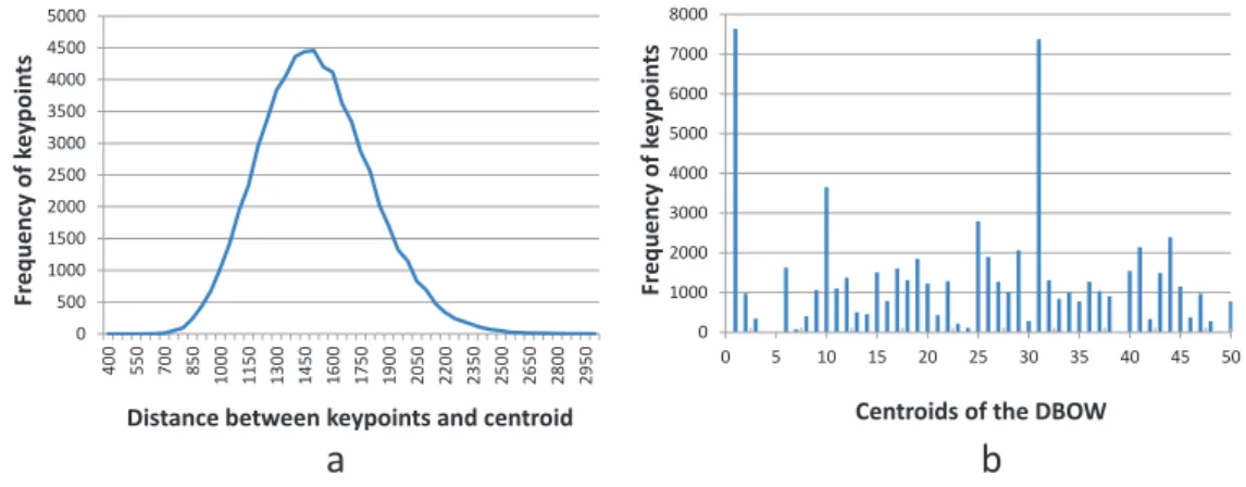
3.7 Distribution of Difference vectors in a Voronoi cell: (a) magnitude of Difference vectors, (b) quantized over a 50-centroid global difference dictionary . . . 41
3.8 Representation of BOW and DBOW . . . 42
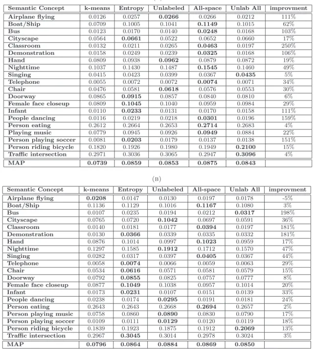
3.9 Concept scores for TRECID 2007: increase/decrease in Average Precision score over the baseline for the best performing HE similarity and DBOW methods for the 3 base dictionary sizes. . . 46
3.10 Concept scores for TRECID 2010: increase/decrease in Average Precision score over the baseline for the best performing HE similarity and DBOW methods for the 3 base dictionary sizes. . . 48
4.1 Single Label Learning Paradigm or One vs. All Learning . . . 49
4.2 Single Label learning vs Groups of Labels learning . . . 50
4.3 Single Label learning vs Groups of Labels learning . . . 52
4.4 M matrices for 4-class ECOC representations: (a) Binary ECOC design. The codeword for the new predicted example x is closest to class having label l2. (b) Ternary ECOC design where the gray entries correspond to the 0 in the dichotomies. Here x is assigned the label l1 based on hamming distance. . . . 57
4.5 Grouping of concepts into non mutually exclusive partitions: a) A simplified space is shown with some labeled (and multi-labeled examples. b) Grouping of concepts. Concepts may appear in multiple groups. c) Each concept is a
unique bit string and no group is empty. . . 60
4.6 Average visual features and the induced visual space.. . . 61
4.7 Clever grouping when then number of groups is less than the number of concepts. 62 4.8 Clever grouping when then number of groups is greater than the number of concepts. . . 63
4.9 Mean Average Precision for 50 concepts for different grouping criteria and their fusion with the baseline. . . 66
4.10 Evolution of the fusion weights with the increase in the number of groups. . . 67
4.11 ECOC construction. . . 73
4.12 Find the distortion within a partition of labels . . . 74
4.13 ECOC matrix generated for TRECVID 2010 dataset with λ = 0. . . 77
4.14 ECOC matrix generated for TRECVID 2010 dataset with λ = 1. . . 78
4.15 Average Precision for 50 concepts: Ensemble of 6 ECOCs, TRECVID 2010. . 81
4.16 Average Precision for 38 concepts: Ensemble of 6 ECOCs, TRECVID 2013. . 82
4.17 Node Splitting Algorithm . . . 85
4.18 A binary tree which partitions the label-set and the corresponding M -matrix with 3 dichotomies. Each node of the tree represents a column of the M-matrix 87 4.19 AP scores for 10 concepts with fewest positive annotations in TV2010 . . . . 90
4.20 AP scores for 10 concepts with fewest positive annotations in TV2013 . . . . 91
4.21 TRECVID 2010 (50 concepts). Performance (MAP) comparison of proposed label partitioning to random partitioning and single label classification, for various groups of trees.. . . 92
4.22 TREVID 2013 (38 concepts). Performance (MAP) comparison of proposed label partitioning to random partitioning and single label classification, for various groups of trees.. . . 92
5.1 Selective Multi Cotraining: Identifying the best view at each iteration for retraining from a choice of views . . . 100
5.2 Selecting source view for Selective Multi Cotraining methods and adding new examples to the training set. . . 101
5.3 Linear fusion of every pair of descriptor for different methods . . . 105
B.1 D´etection de concept dans une vid´eo . . . 122
B.2 Le pipeline de d´etection. . . 124
B.3 L’extraction des caract´eristiques locales et globales. . . 124
B.4 Codage et agr´egation des caract´eristiques de bas niveau pour g´en´er´e un de-scripteur resum´e de l’image. . . 126
B.5 (a) Un classificateur discriminatif distinguant les exemples positifs et n´egatifs. (b) Un classificateur generatif adapt´e `a la distribution des exemples positifs. . 127
B.6 La fusion pr´ecoce et tardive . . . 128
3.1 Mean Average Precision for 20 concepts for baseline (K-means) and three entropy minimization based mapping criteria. Min Ent: Concept distribution Entropy Minimization, Cd: Concept Dependent Entropy Minimization and
Cd (Av): Average Concept Dependent Entropy Minimization. . . 35
3.2 Mean Average Precision for 20 concepts using three alternatives of the concept distribution entropy minimization based mapping. Unlab: Inclusion of the unlabeled examples, All Space: Allow merging of non-contiguous cells and Unlab All Space: Non-contiguous merging allowed with unlabeled examples. 37 3.3 Upperbounds of concept-wise improvements for dictionaries of (a) 500 visual words and (b) 1000 visual words . . . 38
3.4 Comparing MAP for 20 concepts using three large dictionaries vs correspond-ing smaller supervised dictionaries of (a) 500 and (b) 1000 visual words . . . 39
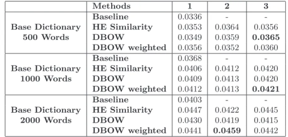
3.5 Mean Average Precision of all methods for 20 concepts (TRECVID 2007) for 3 different dictionary sizes . . . 45
3.6 Mean Average Precision of all methods for 50 concepts (TRECVID 2010) for 3 different dictionary sizes . . . 47
4.1 MAP scores for various ensembles for TRECVID 2010 . . . 79
4.2 MAP scores for various ensembles for TRECVID 2013 . . . 79
4.3 MAP scores for TRECVID 2010 and 2013 . . . 89
4.4 Average number of examples per classifier . . . 89
4.5 MAP scores for all concepts using subsets of concepts for tree generation. . . 90
5.1 Mean Average Precision for various methods for 38 evaluated concepts. Re-sults underlined show statistically significant improvements over the baseline. 104 5.2 Views selected for PRR, precision = 50 . . . 105
5.3 Views selected for PRR, precision = 60 . . . 105
5.4 Views selected for PRR, precision = 70 . . . 106
5.5 Mean Average Precision for the selective multi cotraining methods with the added view based on the caffe1000 descriptor. Results underlined show sta-tistically significant improvements over the baseline. . . 106
5.6 MAP scores for multiview learning techniques for various views (descriptors): (a) k is fixed as the percentage of positive examples of the concept, (b) k is decided based on the precision of the concept classifier on the validation set. 109
Introduction
They say a picture is worth a thousand words but this is a mere understatement in computer vision. In fact, for vision scientists, a picture may contain millions of visual words. These visual words are built using various visual features capturing important measurements from images (color, texture, spatial arrangements, local patches, global statistics, etc. . . ). All this multitude of information is used to help computers capture the understanding of the content of images. It is an attempt to make machines see and understand the world like we do. However this multi-megabytes of information still achieves partial success and the recognition of content in the images continues to elude our intelligent machines.
Video analysis is a scaled-up version of the same problem where a series of images come into play bringing along the relation between frames and temporal dependencies. The core, however, still constitutes of analysis at frame level. Automatic image/video analysis consists of tasks like categorization, retrieval, copy detection, event detection etc., at the helm of which lies the ability to recognize the visual content based on image semantics. Manipulating images and video documents for automatic analysis is among the most difficult challenges
faced in computer vision [1]. However the need for automatic recognition of visual content
has never been felt more strongly before with the exponential increase in the amount of visual information spreading over the internet. Roughly 350 million new photos are uploaded to
Facebook every day [2], and the number for Flickr is between 20 to 40 million per day [3].
Moreover Facebook boasts more than quarter of a trillion photos uploaded to their web site. YouTube has an astounding 100 hours of new video uploaded every minute. The amount of users using these services is growing by day and this online medium of communication is now matching the importance of broadcast Television. This staggering amount of new information and its importance to users calls for reliable and efficient methods to analyze the visual content in order to develop methods to automatically search, index and browse these large databases.
In this introduction we start with explaining the pursued Video Concept Detection task which is also referred to as Semantic Indexing. We follow with an overview of the major
steps involved in achieving concept detection. Further we analyze the opportunities for improvements in the detection pipeline and present our motivations to work in the selected directions. The introduction lists, at the end, our contributions to the video concept detection pipeline.
1.1
Video Concept Detection (Semantic Indexing)
For years scientific research in image and video retrieval and indexing has been dominated by text or concept based approaches where the metadata or associated text based descriptions like title, an article or narrative and tags etc. are used to retrieve multimedia content from the internet. Practically this is the popular method these days to get images from the popular search engines and look for videos on video sharing services like YouTube and Dailymotion. Since the dawn of the century though research focus has been shifted to directly understanding the content of the multimedia documents and using the extracted information to build retrieval models. Textual descriptions associated with or surrounding the multimedia content on the internet are not always reliable. These are usually subjective to the uploader, personalized, misleading, incomplete and sometimes do not exist at all. Moreover annotating a large video database from scratch with manual human effort is laborious and could suffer from the similar incompleteness and bias. The content on the other hand is always right and we can safely rely on its authenticity, provided its correct use.
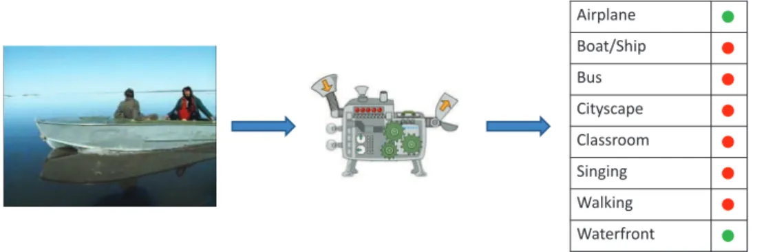
Airplane Boat/Ship Bus Cityscape Classroom Singing Walking Waterfront
Figure 1.1: Video Concept Detection
Video Concept Detection or video categorization aims at automatically describing a video
with semantic concepts that correspond to the content of the video, figure1.1. These
seman-tic concepts are high level descriptions of the video that directly depict the key information present in the content. The semantic concept can consist simply of labels like objects or people, can be depicted by a scene or can comprise of a situation with a complex interaction of different entities. The solution assigns a probability of presence to a concept or a label in the video frame (e.g. the video contains a ”Bus” for sure and is less likely to contain a ”Helicopter hovering”). The probability is assigned by a classifier which is trained for that concept. This classification model is built for each concept separately. The classification is
not done for each frame of the video, rather a set of keyframes are extracted for each video
[4, 5]. These keyframes are representative of the video content. Video is first segmented
into shots where a new shot location can be given with the video metadata or can be
au-tomatically detected [5]. Usually a single keyframe is then extracted from each video shot
which is the most informative of the shot frames. Since analyzing videos with keyframes offer
a convenient and effective alternative to analyzing video as a whole [4–6] we opt to work with
keyframes throughout this thesis.
A semantic concept does not have a fixed description most of the times and there exists plenty of within class variations. The detection framework has to capture this intra-class variability when building classification models for concepts. The video concept detection system which starts to work with the raw pixel data from images and assigns probabilities to test images is very intricate and is composed of quite a few processing steps. These steps are detailed in the next section.
1.2
Video Concept Detection Pipeline
A video categorization system comprises a complex structure of more or less sequential ele-ments which span over a number of scientific disciplines including image and signal
process-ing, statistical analysis, mining and machine learning to name a few. Figure1.2presents the
major components of the framework where we start with images (keyframes) assuming that video was already segmented into shots. Building different concept detection models and using them employs largely all the steps of the framework and only differ in the functionality of some of the stages.
The system extracts a number of different visual features from the provided images at the stage 1 of the framework. These raw features are usually not used directly and are rather transformed to an aggregated image specific representation in the stage 2 of the pipeline for further processing. A number of annotated images is usually available to learn the model which classifies the concept images from the rest. This makes the 3rd stage where the classification model is used to find predictions on the test images which depicts the prospects of existence of the concept in the corresponding video. The fourth stage is an additional but very useful step where predictions from different models are combined to unite the powers of the individual learners. We briefly describe each of the stages of the pipeline below before looking into the possible rooms for improvement in the components of the pipeline.
Stage 1: Feature Extraction and Description
An image in a typical video is composed of tens of thousands of pixels that are mere numerals but an enormous amount of information can be extracted from a single image. This step is the foundation of the detection or retrieval framework as features are expected to capture the essence of what the image represents. Humans can, most of the times, figure out the concept depicted in the image by just taking a look. The features are expected to encapsulate this
Stage 1 Feature extraction
from key image locations - - - - - - - - - - - - - - - - - - - - - - - - - - - - - - High dimensional descriptors Stage 2
Feature coding and pooling
Universal Representation Model
pooling
One Feature Vector
Stage 3 Model Learning Learner Stage 4 Model fusion Training images
Training image vectors
New Image
Fusion Module
Most likely label(s)
Most likely label(s)
Figure 1.2: Video Concept Detection Pipeline.
essence of the image for machines. They capture the semantics of the image to make the machine understand the similarity or dissimilarity between the images.
A video frame can be described globally or can be bisected into regions before building descriptions for each region. These descriptors are called the visual features of the image. While global features capture the qualities or properties of the image on the whole the local features work on a local neighborhood of the image to gather information about the targeted pixel. Global features can be computed for the whole image or parts of image by first segmenting the image into predefined parts and then building the feature for each segment. They describe global properties of the image (segment) like color, gist or some sort of spacial information. Local features may be described for predefined image locations and are sometimes only extracted for specific image points. These points are expected to contain rich information compared to the rest of the image. Methods are employed to find these critical points that are based on some maximization criterion. Statistics from the local
Global and local image descriptors - - - - - - - - - - - - - - - - - - - - - - - - - - - - - - - - - - - - - - - - - - - - - - - - - - - - - - - - - - - - - - - - - - - - - - - - - - - - - - - - - - - - - - - - - - - - - - - - - - - - - - - - - - - - - - - - - - - - - - - - - - - - - - - - - - - - - - - - - - - - - - - - - - - - - - - - - - - - - - - - - - - - - - - - - - - - - - - - - - - -
Image processing and statistical analysis tools Input image
Figure 1.3: Global and local feature extraction example.
neighborhood or patch are calculated to describe that part of the image. The number of features thus may vary from image to image if this kind of patch extraction is done. Local statistics include extracting properties like information about shape and geometry, the local
structure, texture etc.. Figure 1.3 depicts the idea of extracting global and local features
from an example image. Note that size and number of features extracted are different for different feature types.
The features extracted should be relevant to the specific task of concept detection and should be robust. So if the appearance of e.g. an object changes in the image the features should still be able to capture the relevant and necessary information. They should also resist change to the accidental distortion of images from illumination variation, camera movement and other forms of distortions. A good knowledge of image processing is required to build such features.
Usually the features of a specific type are used to build the rest of the system but sometimes different types of features can be merged pre-hand to perform the task. More discussion on the use of the features is to follow.
Stage 2: Feature Coding and pooling
The different kinds of features extracted in the previous stage can be directly used to represent an image but their use is prohibitive due to their sheer size and huge number. This is more often the case for local image descriptors that are extracted at numerous image locations. Furthermore the number of these features extracted from the images could be different as well which prohibits a unified representation for all the images. That is why the features are
usually summarized into a single high dimensional feature vector of fixed length, figure 1.4.
To construct the unified representation first the features from the image are transformed or coded into a set of values. This projection of the feature onto the new representation has certain properties: two features that are close are encoded into the same representation,
- - - - - - - - - - - - - - - - - - - - - - - - - - - - - - - - - - - - - - - Coding Pooling
Projecting the descriptors into the coded space Aggregating the projections to aquire a fixed length feature
Figure 1.4: Coding and pooling to generate the summarized feature for an image.
of coding include vector quantization [8], soft assignment [9, 10] and probability
estima-tion for GMMs to generate Fisher vectors [11]. The new representation or the codebook is
constructed using features from some training images. After each image feature is coded, pooling aggregates the coded features into a single value for each of the codes. This results in a vector of values with length equal to the number of coded representations. Pooling can vary from averaging and taking the maximum value to parameter adaptation in the case of
Fisher vectors [11,12].
The benefit of these fixed length vectors is that they can be directly fed into a discrimi-native classifier and a model for the concept can be built. Moreover the reduced size helps in fast learning and efficient prediction of the test examples. On the other side of the pic-ture the true discriminative power of the feapic-tures that cappic-ture the image dynamics from specific locations is somewhat lost as the local features are aggregated. Extreme values may be diminished due to averaging or maximizing and geometrical structure can be no longer used. Refinements can be done to include some useful information that hints at some of the lost dynamics of the original image. The size of the coded representation can be increased to better distinguish the image features at the expense of increased training and prediction time and the risk of overfitting the parameters to the training images.
Stage 3: Model Learning
This stage is the brain of the pipeline where machine learns to correctly identify examples of a concept. This necessitates the presence of some annotated images that must be used for learning the model for a semantic concept. These images are treated as the positive examples and are used to train the classification model to distinguish them from the rest of the world. To be able to achieve this intelligent behavior a great deal of number crunching is required and usually this step takes the most of the time in the pipeline. This time increases linearly with the number of concepts as in practice a separate model is learned for each concept.
State of the art in learning such kind of a model is mainly divided into two parallels:
A discriminative classifier A generative classifier - - - - - - - - - - - - - - - - - - - - - - - - - - - - - - - - - - - - - - - - - - - - - - - - - - - - - - - - - - - - - - - - - - - - - - - - - - - - - - - - - - - - - - - - - - - - - - - - - - - - - - - - - - - - - - - - - - - - - - - - - - - - - - - - - - - - - - - - - - - - - - - - - - - - - - - - - - - - - - - - - - - - - - - - - - - - - - - - - - - - - - - - - - - - - - - - - - - - - - - - - - - - - - - - - - - - - - - - - - - - - - - - - - - - - - - - - - - - - - - - - - - - - - - - - - - - - - - - - - - - - - - - - - - - - - - - - - - - - - - - - - - - - - - - - - - - - - - - - - - - - - - - - - - - - - - - - - - - - - - - - - - - - - - - - - - - - - - - - - - - - - - - - - - - - - - - - - - - - - - - - - - - - - - - - - - - - - - - - - - - - - - - - - - - - - - - - - - - - - - - - - - - - - - - - - - - - - - - - - - - - - - - - - - - - - - - - - - - - - - - - - - - - - - - - - - - - - - - - - - - - - - - - - - - - - - - - - - - - - - - - - - - - - - - - - - - - - - - - - - - - - - - - - - - - - - - - - - - - - - - - - - - - - - - - - - - - - - - - - - - - - - - - - - - - - - - - - - - - - - - - - - - - - - - - - - - - - - - - - - - - - - - - - - - - - - - - - - - - - - - - - - - - - - - - - - - - - - - - - - - - - - - - - - - - - - - - - - - - - - - - - - - - - - - - - - - - - - - - - - - - - - - - - - - - - - - - - - - - - - - - - - - - - - - - - - - - - - - - - - - - - - - - - - - - - - - - - - - - - - - - - - - - - - - - - - - - - - - - - - - - - - - - - - - - - - - - - - - - - - - - - - - - - - - - - - - - - - - - - - - - - - - - - - - - - - - - - - - - - - - - - - - - - - - - - - - - - - - - - - - - - - - - - - - - - - - - - - - - - - - - - - - - - - - - - - - - - - - - - - - - - - - - - - - - - - - - - - - - - - - - - - - - - - - - - - - - - - - - - - - - - - - - - - - - - - - - - - - - - - - - - - - - - - - - - - - - - - - - - - - - - - - - - - - - - - - - - - - - - - - - - - - - - - - - - - - - - - - - - - - - - - - - - - - - - - - - - - - - - - - - - - - - - - - - - - - - - - - - - - - - - - - - - - - - - - - - - - - - - - - - - - - - - - - - - - - - - - - - - - - - - - - - - - - - - - - - - - - - - - - - - - - - - - - - - - - - - - - - - - - - - - - - - - - - - - - - - - - - - - - - - - - - - - - - - - - - - - - - - - - - - - - - - - - - - - - - - - - - - - - - - - - - - - - - - - - - - - - - - - - - - - - - - - - - - - - - - - - - - - - - - - - - - - - - - - - - - - - - - - - - - - - - - - - - - - - - - - - - - - - - - - - - - - - - - - - - - - - - - - - - - - - - - - - - - - - - - - - - - - - - - - - - - - - - - - - - - - - - - - - - - - - - - - - - - - - - - - - - - - - - - - - - - - - - - - - - - - - - - - - - - - - - - - - - - - - - - - - - - - - - - - - - - - - - - - - - - - - - - - - - - - - - - - - - - - - - - - - - - - - - - - - - - - - - - - - - - - - - - - - - - - - - - - - - - - - - - - - - - - - - - - - - - - - - - - - - - - - - - - - - - - - - - - - - - - - - - - - - - - - - - - - - - - - - - - - - - - - - - - - - - - - - - - - - - - - - - - - - - - - - - - - - - - - - - - - - - - - - - - - - - - - - - - - - - - - - - - - - - - - - - - - - - - - - - - - - - - - - - - - - - - - - - - - - - - - - - - - - - - - - - - - - - - - - - - - - - - - - - - - - - - - - - - - - - - - - - - - - - - - - - - - - - - - - - - - - - - - - - - - - - - - - - - - - - - - - - - - - - - - - - - - - - - - - - - - - - - - - - - - - - - - - - - - - - - - - - - - - - - - - - - - - - - - - - - - - - - - - - - - - - - - - - - - - - - - - - - - - - - - - - - -
Figure 1.5: (a) A discriminative classifier separating positive and negative examples. (b) A generative classifier adapted to the positive concept examples.
to map the input examples x to the class labels y [13]. This is achieved by modeling the
conditional probability P (y|x) directly from the input examples x and their respective labels y. On the other hand the Generative classifiers learn the joint probability distribution P (x, y). Bayes Rule is used to find the conditional probability P (y|x) to predict the most likely label. So to resume a generative model tries to learn how the data was generated, and can be used e.g. to generate more samples of the data, while the discriminative model does not care about the data generation and learns to categorize directly.
The quality of the classifier learned depends not only on the type of learning method used and its parameters but also on the kind of feature representation selected and the quality of positive and negative instances acquired for training.
We will give some examples of popular generative and discriminative models used in the concept detection and retrieval frameworks in the next chapter where we discuss state of the art but in this thesis we stick to discriminative form of classification. Stage 4: Fusion Although the concept detection pipeline pretty much completes at the previous step, com-bining a variety of learners on different descriptors is always a fruitful option. Fusion allows learners to be built for different types of features independently and only then be combined when generating the final output concept probability. The different types of features can include other modalities like audio and textual information along with visual features. This type of fusion is called decision or late fusion as it is done at the decision level as shown in
the figure1.6. A feature level fusion can also be envisaged and pops up in the literature now
and then but is less popular due to the heterogeneous combination and the increased size of
the combined feature. Chapter 5 highlights some important contributions from the field of
multimodal fusion.
Finally a feedback loop is employed sometimes to refine the set of training examples and add some new useful examples to build a stronger classification model.
Feature Extraction Feature Extraction Feature Extraction Classifier 1 Classifier 2 Classifier n D eci s io n Fu s io n Final Decision
Figure 1.6: Classifier fusion at the decision level.
1.3
Motivation
The information extracted from video frames at pixel level are low level descriptions of the image and this does not translate directly to the semantic meaning of the image. There exists
thus a Semantic Gap [14] between the low level image description that the computer vision
system uses, to learn about the higher level semantics that the image represents. There are various reasons for the existence of this gap. Foremost is the difference in the human per-ception of a concept and the representation suitable for our computers to understand. Then
there is subjectivity [15, 16], i.e. when different users perceive similar content differently.
Lastly the semantic gap is widened by the within class diversity for many concepts. To highlight this problem consider an image of a chair placed inside an office and another image of a chair outside in a lawn. Though both images contain the concept Chair, the low level pixels would not agree for the most part of the two images. Research in automatic video content understanding has been focused to reduce this semantic gap.
The performance of a detection system depends on all the factors that make up the detec-tion pipeline. For each of these steps we list below the main opportunities of improvement.
• Features extracted at pixel level
As the basis of the detection pipeline this phase receives considerable research attention in order to capture the most useful information with a manageable size from the images. • Selecting and building the most informative mid-level representation
Summarizing the visual features is the most sensitive step in the pipeline as most of the raw low level information is lost here. Research in this area focuses on building comprehensive mid-level representations that successfully capture the image semantics. • Refining the representation
Research has also been done to refine the mid-level representation to try to bridge the semantic gap by adding e.g. contextual, spatial or label specific information.
• Quality of annotations/ selecting the best examples
The tedious work of extracting and summarizing features is of no use if representative examples are not used for concept model learning. Selecting the best examples for training and refining them with feedback is important to the performance of the system. Moreover there always exist great amount of unlabeled examples to be discovered. New instances should be added to add diversity while increasing performance.
• Finding the best decision boundary
In the end it all comes to the classifier which distinguishes the positive instances from the negatives. Research is evolving in this area as well to build classifiers that generalize well on test examples and have lower complexity.
• Fusing the best classifiers effectively
Research continues to find new methods to select the best classifiers among the pool of multimodal classifiers and combine them in the most effective way.
1.3.1 Making the Slice Bigger
With the enormous amount of visual information extracted from the images, the various coding and pooling methods and the variety of strong classification techniques available, not everything is used to build the categorization system. If too many features or parameters are used to train the models for concepts there is a risk of overfitting on the training examples. Moreover this would require loads of computing power and time as the feature representations are high dimensional and the current processing power limits the extravagance use of this visual information.
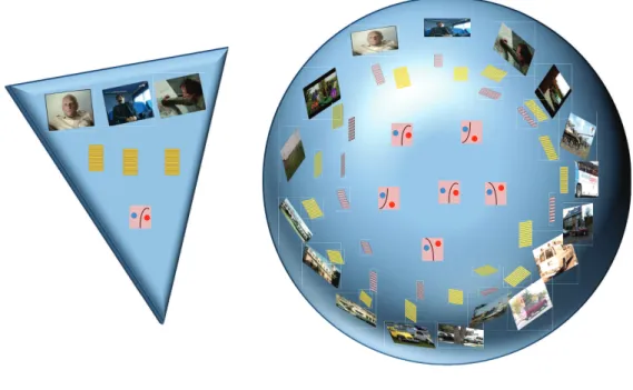
We can look at all this information as making a Visual World, figure 1.7, and usually a
video concept detection system only takes a slice of this world with a number of annotated images, certain features and a classification algorithm that learns a model using this informa-tion. The amount of information going into the slice goes from raw image level information to classification decision which justifies the pyramidal structure. What we target in this thesis is how to make this slice bigger by exploring the Visual World in order to add extra and useful information with little effect on complexity of the task to improve video concept detection. So instead of cutting the standard slice from the Visual World we cut a bigger slice where we include additional information at various levels of the concept detection pipeline
1.2. Note that in terms of this Visual World, classifier fusion can be regarded as combining
- - - - - - - - - - - - - - - - - - - - - - - - - - - - - - - - - - - - - - - - - - - - - - - - - - - - - - - - - - - - - - - - - - - - - - - - - - - - - - - - - - - - - - - - - - - - - - - - - - - - - - - - - - - - - - - - - - - - - - - - - - - - - - - - - - - - - - - - - - - - - - - - - - - - - - - - - - - - - - - - - - - - - - - - - - - - - - - - - - - - - - - - - - - - - - - - - - - - - - - - - - - - - - - - - - - - - - - - - - - - - - - - - - - - - - - - - - - - - - - - - - - - - - - - - - - -
Figure 1.7: The Visual World with numberous images, feaures and classifiers.
1.4
Our Contributions
Our contributions target two major areas of the concept detection pipeline: feature coding and pooling, and Model learning where we focus on finding useful training examples. The following paragraphs summarize our contributions.
• We use state of the art features extracted from the images and work on their transfor-mation into the mid-level representation. We use label infortransfor-mation while building this representation in order to add some image and concept specific information into the feature.
• We also enhance the standard image representation by encoding the feature with trans-formation specific intrans-formation.
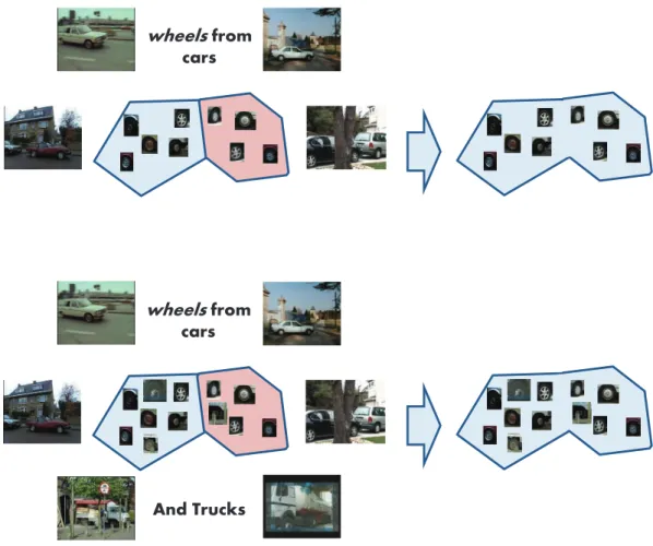
• To improve the classification performance for a concept we explore examples of other related concepts in order to add useful and diverse information. The idea is that common or close concepts share information among themselves and it should be put to use when learning the classification models.
• We extend the idea above to look at concepts that are not so close, rather that are different, to learn from the dissimilarity between concepts.
• Finally we try to explore the unlabeled examples in a semi supervised setting to increase the amount of annotated data and use the best information out of it to learn the concept models.
This concludes the introductory chapter of this manuscript which is followed by a brief
review of the state of the art methods in video concept detection and retrieval in chapter 2.
We limit our discussion to methods important to the concept detection pipeline. Each of the rest of the chapters also include some review of popular methods as it makes more sense to
describe the work that inspired us with the corresponding contributions. Chapter3includes
the first of our contributions where we try to improve the mid-level video representation. In
chapter 4 we base our work on the similarities and differences between concepts to try to
find useful new examples to perform improved concept detection. Chapter 5 explores the
unlabeled examples and presents criteria to select the most useful new examples. Finally in
chapter6we summarize our contributions and draw conclusions. We also list possible future
avenues to explore for automatic analysis of video content especially leading to video concept detection.
State of the Art
Automatic analysis of video content is among the hardest problems faced by the computer vision and multimedia community. It receives a significant amount of dedicated research attention from academic and industrial research teams all over the globe due to its importance in the growing digital world. As pointed out in the introduction the research in this field is truly interdisciplinary and integrates works ranging from image and signal processing to statistical machine learning. Consequently it is imperative to review the state of the art in the vast field of visual content analysis specifically targeting video concept detection and retrieval. This chapter lists important contributions to each of the stages of the concept detection pipeline starting from raw feature extraction to fusing the high level decisions.
In the early 90s with the advent and increase of digital media and the availability of cheap
media capturing devices research interest grew in the content based retrieval field [14,16,17].
Research exploded after the dawn of the millennium when Google launched its text based image search. It was evident that directly understanding the content of the images was the new target. Around the same time National Institute of Standards and Technology (NIST) also jumped into the action and later in 2003 formed a dedicated research track allocated to
video analysis based techniques called TRECVID [18].
In terms of scalability of the content based image/video search problem the databases
used have literally gone from indexing thousands [19, 20] to millions [12, 21–25] and now
billions [26] of images in the last 20 years [17].
In the year 2000 Smeulders et al.[14] presented a review on content based image retrieval
citing about 200 references. The problem of automatically understanding the visual content has received continued attention in the last 14 years with thousands of available works and many dedicated conferences and workshops. We only select some of those works that we feel are the most representative and cover more or less the stages of the concept detection
pipeline presented in the figure1.2.
2.1
Feature Extraction
Visual feature extraction converts an image to a mathematical representation and it forms the basis of any visual content analysis system. The features should capture enough informa-tion to differentiate the class instances from the non-class instances. Since the features are extracted from raw pixel values this step is susceptible to noise that may come from camera motion, variations in lighting, change in scale and viewpoint, occlusions, lower resolution, quality of the frame extracted or the movement of the objects in the frame themselves. The features extracted in this stage should be robust to all these noise and variations and should be compact. There is no winner when it comes to capturing the visual information due to the complex composition of data, the intra class diversity and the nature of the semantic concept to be detected. The features or image descriptors are mainly divided into two types: global and local features.
2.1.1 Global Features
Global features describe the properties of the image as a whole summarizing the information into one compact description. They are faster to compute and are highly scalable compared to their counterpart but lack enough discriminatory information. Color seems to be an important and intuitive global choice when trying to predict the semantic concept in an image. Globally dominant colors can give indications about the concept like if an image
contains large components of blue and green it is likely to be an outdoor scene [27].
This is precisely true as color features have been there since the conception of the field of image analysis and are being used till date. The most straightforward use of color
is in building the color histograms from the pixel values in the RGB space [28, 29]. To
make the color histograms invariant to changes in light intensity and shadows, normalization
is performed [30, 31]. Color spaces other than the omnipresent RGB have also been used
explicitly. Weijer et al. [32] build color histograms in the HSV space where the H bins are
weighted by the saturation making the representation robust to changes in scale and shift.
Hays and Efros [33] use the L*a*b* space to build 784 dimensional histograms with 4, 14
and 14 bins in the L, a and b respectively. Chang et al. [34] build a 12 bin histogram for 11
colors and one outlier bin. They extend their feature by building histograms for each color
at finer resolutions along with mean and variance of the HSV channels. [35] extracts average
color components of the LUV space (L:luminance, UV chrominance) of 16 pixels from the image divided into 4 X 4 blocks.
Color moments [36–38] are defined on the distribution of the RGB triplets. These are
usually extracted up to the 2nd order, are rotation invariant and higher order moments also contain spatial information. Color map reflects the user’s search intention with a small feature by allowing the user to indicate the spatial distribution of colors in the desired images
Holistic representations capture dominant spatial structure of a scene into a low
dimensional feature from a scaled down image [24]. Olivia and Torralba [40] proposed the
GIST feature which summarizes Gabor filter responses, which was further compressed using
different strategies [23,41]. GIST features have also been extracted from image regions by
accumulating responses from filters at different orientations and scale [33,42].
Texture features capture important properties like smoothness, coarseness or some pat-tern that occurs repeatedly throughout the image. Pioneer textural features were extracted
by Tamura et al. [43] emulating the human visual perception. For outdoor scenes textural
properties might be geographically correlated [33] e.g. the building in a city’s skyline or
vegetation. A universal texton dictionary is a popular method that summarizes the pixel
responses to a bank of orientation filters [33,44, 45]. [34] decomposes each image into four
sub-images using discrete wavelet transform and build nine texture features with different
compositions of the decomposed images. Li and Wang [35] perform Haar transform on the L
component of the LUV image space for each 4 X 4 block of the image. They use average of the 3 out of 4 wavelet components to build their feature containing 3 values for each 4 X 4 block. Recently discriminatory texture information is also extracted using Local Binary
Pat-terns (LBP) from image patches and aggregating them into a global descriptor [46]. LBP is
extended by considering the distance between the center pixel and its neighbor for improved
image retrieval [47] but with a higher dimensional feature. More recently [48] has extracted
LBP for different color spaces.
Global edge distribution is another important piece of information gathered from im-ages. Like color, edge histograms are the simplest representation capturing cumulative edge
orientation information in images [49]. Wang et al. [50] build a global edge descriptor
concatenating histograms from 5 over-lapping image regions.
2.1.2 Local Features
Global image descriptors sometimes do not capture the spatial relationship between image objects, often carry redundant information and are usually not invariant to photometric and geometric distortions. Local features are described at key image locations or interest points
that are identified in the image and supposedly carry valuable local information [51]. These
points can be predefined though, e.g. in the form of a dense grid over the image [52–57].
The descriptor then calculates statistics based on the local neighborhood usually depicting the shape of the region.
The purpose of keypoint detection is to sample a sparse set of regions in the image that are invariant to geometric and photometric transformations. SIFT (Scale Invariant Feature Transform) detects interest points using Difference of Gaussian (DoG) operator but is only partially invariant to illumination changes and affine transformations. More robust detectors
(MSER) detector [59] and [60] based on image edge and intensity based region detection.
SURF (Speeded Up Robust Features) [61] detects interest points using a Hessian-Laplace
based detector working on integral images to reduce detection time.
The SIFT descriptor [62, 63] posed as a breakthrough in describing local regions and
is one of the most frequently occurring descriptors in research works to date. The feature induces a histogram on a local image region that was first detected using DoG operator and then described in terms of 8 dominant orientations of the gradient. The gradient is calculated in the neighborhood of 4 X 4 spatial grid and is thus a 128 dimensional feature. SIFT is robust to geometric and photometric transformations and is invariant to scaling, translation and rotation of the image. Gradient Location and Orientation Histogram (GLOH) extends SIFT to a 272 dimension histogram computing the descriptor for a log-polar location grid
[58]. PCA-SIFT [64] increases the efficiency of retrieval by reducing the dimensions of the
SIFT feature, while SURF [61] estimates the dominant orientation of the interest point
neighborhood and accumulates the horizontal and vertical wavelet responses (w.r.t. the dominant orientation) of 16 regions around the interest pixel resulting in a 64 dimensional feature. Finally using a power normalization on the SIFT has also proven to be affective as
in [65] and RootSIFT [66] where square rooted SIFT descriptors are stored.
Dalal and Triggs [67] came up with the Histogram of Oriented Gradients (HOG)
descrip-tor which is among the most successful features used for visual recognition. HOG mainly follows SIFT methodology and captures the local distribution of edge orientations where the location information is generally lost. The descriptor aggregates the edge orientations of lo-cal patches that are regularly spaced into a histogram. Several extensions and improvements of HOG have also been successful where the feature is calculated on variable sized regions
[68], calculated from segmented foreground and background images [69] and from signed and
unsigned gradient information [70]. [71] also augment the high resolution local HOG feature
with LBP statistics.
2.2
Feature Coding and Pooling
Local features capture discriminatory visual information from all over the image but they are mostly not used directly for image categorization. The low level descriptors are summarized into an intermediate representation usually through a two-step coding and pooling method. There is an unspoken rule for the successful working of such a representation: similar images should have similar representations but it should be discriminative enough to distinguish from instances of other classes. The low level visual information is somewhat lost but the new representation is compact, is of fixed size and is more robust to descriptor noise and small transformations in the image which helps the model to be generalized to test images. This intermediate representation encoding local visual characteristics is closer to the human
The breakthrough for representing visual information was achieved when vector
quan-tization was used to build the Bag of Words (BOW) model [8, 20]. A universal codebook
or visual dictionary is build using features from the training images by unsupervised vector quantization. Features are coded to the nearest code or visual word. Sometimes only the
most informative features are used to construct the dictionary [73]. Average [8,20] or max
pooling [74, 75] is used to build the mid-level BOW feature vector. Multiple assignments
encodes a visual feature as belonging to the k nearest visual words. Soft assignment further relaxes the coding process and probabilistically assigns a feature to the closest visual words
[9,10,76]. It can be seen as assigning a weight to each encoded feature. However authors in
[77] revert back to assigning a local feature to a single visual word with a degree of
partici-pation, that is calculated based on the previous assignments of local features to that visual word.
Grauman and Darrell [78] presented a multi-resolution histogram to encode local features
with out using a universal dictionary. The Bag of Words or Bags of Features models are orderless and do not contain any spatial or structural information about the image. Lazebnik
at al. [54] inducted spatial information into the BOW framework by building histograms
for specific image regions, which they named Spatial Pyramid Matching. Each feature is coded and pooled for each of the histograms and one representation is build for the image
accumulating all the histograms. Locality-constrained Linear Coding (LLC) [74] improves
the spatial pyramid approach by encoding each descriptor into a projected local coordinate
system with a different basis. Sparse Coding [7, 79] also provides an alternative to vector
quantization by relaxing the cardinality constraint and removing the extreme sparseness of the representation. Sparse coding is more general and is ironically usually less sparse than a vector quantized representation. Both these works use max pooling to obtain state of the
art image classification results. Boureau et al. [80] use local pooling in the feature space to
avoid different features encoded with the similar code (vector quantized, sparse coded) to be pooled together.
The research in image representation is further carried to build higher level representa-tions where visual words are supposed to co-occur for certain objects or concepts. Considering different visual words as a single unit will reduce ambiguity that may arise when different intended meaning of visual words are considered. This notion of inter-relation is captured
in terms of visual phrases [81, 82] which consist of more than one visual words and help
distinguish the object from non-class instances which do not contain those specific visual words.
Recently effective techniques have been shown to improve image retrieval by aggregating
element wise differences of local descriptors [25] and aggregating Tensor products of those
differences [83]. This results in a larger feature vector for a small visual codebook
captur-ing important statistics about the distribution of the descriptors inside the clustercaptur-ing cell. The more general Fisher Vectors have been shown to capture vital higher level descriptors
distribution statistics for visual recognition tasks [11,12]. First the global density of the dis-tribution of image descriptors is estimated using Gaussian Mixture Models (GMMs) trained on all the descriptors from the training images. An image signature is then calculated in terms of Fisher Vectors which indicate the direction in which the parameters of the image model to be changed in order to best fit the global distribution. The GMM can be regarded as a generative visual dictionary and each Gaussian is considered a visual word. Supervectors
[84] work with a similarly trained GMM on the image features and encodes the first order
difference with the mean of the cluster with the image representation.
2.3
Classification
The problems of video concept detection and video/image retrieval generally fall under the paradigm of supervised learning where a number of annotated image instances are available to build the model for each semantic concept. The learned model is trained on the ground-truth images to classify new instances as belonging to the class or not. Supervised classification methods are divided into two broad categories; Generative Classifiers, which learn the joint probability distribution of the training examples and the outputs for each class and apply Bayes’ rule to predict the class probability of the new instance, and Discriminative Classifiers, which directly learns the classification boundary using examples from both class and non-class instances. We briefly review some of the popular methods for both the categories in the sections that follow.
2.3.1 Generative Models
Generally once the joint probability is modeled maximum a posteriori (MAP) or maximum likelihood (ML) estimates are used to find the candidate class(es) for the new image. Some pioneering works in image classification directly employed Bayesian classification to classify
images into indoor and outdoor scenes [85,86]. [85] further classifies outdoor images as city
and landscape and continues to classify landscape images into sunset, forest and mountain.
Mori et al. [87] use a co-occurrence model to find the correspondence between image features
and the text keywords. A more robust idea is to find the correspondence between test image
and the labeled images using e.g. Cross Media Relevance Modeling (CMRM) [88]. The
keywords associated with the labeled images are used to annotate the test image. Huang et
al. [89] combine CMRM with other correspondence models to improve image annotation.
Another direction is to include latent variables in the model to associate visual features with
keywords, referred to as latent Semantic Analysis (LSA) or probabilistic LSA (pLSA) [90,91].
GMMs are also used to model the distribution of visual features [92,93]. Blei and Jordan
[94] assumed a Dirichlet distribution is used to create the mixtures and used Latent Dirichlet
Allocation (LDA) to generate the distribution of visual features and keywords. Fei Fei and