Scheduling of heat integrated multipurpose batch Processes

To cite this version :

Hétreux, Gilles

and Ramaroson, Anthony

and

Duquenne, Philippe

Scheduling of heat integrated multipurpose batch

Processes. (2011) In: XIIIème congrès de la SFGP Des procédés au service

du produit au coeur de l'Europe, 29 November 2011 - 1 December 2011

(Lille, France).

O

pen

A

rchive

T

OULOUSE

A

rchive

O

uverte (

OATAO

)

OATAO is an open access repository that collects the work of Toulouse researchers and

makes it freely available over the web where possible.

This is an author-deposited version published in :

http://oatao.univ-toulouse.fr/

Eprints ID : 20178

To link to this article:

URL

:

http://www.sfgp.asso.fr/publications/collection-recents-progres-en-genie-des-procedes/

Any correspondence concerning this service should be sent to the repository

administrator:

staff-oatao@listes-diff.inp-toulouse.fr

Scheduling of Heat Integrated Multipurpose Batch Processes

HETREUX Gilles*, RAMAROSON Anthony, DUQUENNE Philippe LGC (UMR CNRS 5503) – Dpt Procédés et Systèmes Industriels

4, allée Emile Monso, 31030 TOULOUSE

Abstract

A systematic mathematical framework for scheduling the operation of multipurpose batch plants involving heat-integrated unit operations is presented. The approach advocated takes direct account of the trade-offs between maximal exploitation of heat-integration and others scheduling objectives and constraints. In this paper, heat transfer takes place directly between the fluids undergoing processing in the heat integrated unit operations, and therefore a degree of time overlap of these operations must be ensured. The modelling is based on the ERTN formalism and a discrete time MILP formulation.

Key-words : Scheduling of batch processes, heat integration, ERTN modeling, MILP formulation.

1. Introduction

Recent works have highlighted the need for efficient utilization of energy in the operation of batch plants. However, in contrast to the extensive amount of work already published on energy integration in continuous plant, relatively little has been reported in the literature on this aspect of the operation and design of flexible multipurpose batch plants. The majority of studies are based on the concept of pinch

(Linnhoff et al, 1988), modified in order to accommodate the complications introduced by the time-varying operation of batch processes (Time Average Model). Despite its clear importance, the minimization of the cost of external utilities consumed is not usually the primary objective in scheduling the operation of a multipurpose plant. This is the consequence partly of the paramount demand for timely satisfaction of the multiple production requirements imposed on these plants and partly of the often small proportion of energy costs compared to the high value of the raw material and products produced in many such plants (e.g. ., in the pharmaceutical industry). It could, therefore, be argued that optimizing the exploitation of any heat integration opportunities afforded by a fixed production schedule that already achieves all other plant objectives is indeed a reasonable approach.

In general, even optimal production schedules tend to be quite degenerate, in the sense that there often exist a large number of different schedules, all of which can achieve a given set of production requirements. However, the potential for heat integration could vary significantly from one such schedule to another. Furthermore, in some industrial sectors (e.g. food, diary, brewing) that employ multipurpose plants, energy costs do form a significant proportion of the total production cost, and thus have to be balanced properly against other costs, such as those of the raw materials and manpower, and the value of the products. On the basis of the above discussion, heat integration must be considered as an integral part of the problem of scheduling the production in a given plant, with the cost of utilities incorporated within the overall economic objective.

In this context, this paper proposes a systematic mathematical framework for the exploitation of heat integration in batch plant operation. The rest of this paper is organized as follow. The next section introduces briefly the ERTN formalism and describes the modeling of direct heat integration mode. Then, Section 3 provides a brief review of the proposed formulation. Finally, an example of a heat-integrated process is used to illustrate the approach in section 4.

2. A graphical modelling framework : the Extended Resource Task Network

Among the available CAPE tools (Computer Aided Process Engineering), process engineers are showing a growing interest in scheduling methods based on MILP formulation in order to carry out various performance analyses such as system productivity, time cycle, production costs or energy efficiency of a *

Axx-2

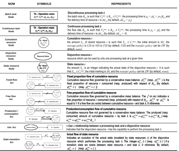
unit. Nevertheless, the implementation and the tuning of a MILP model can become rather technical and complex in some cases. To facilitate the modelling phase by non-expert users in optimization, a way is to build mathematical models which are structurally generic and configurable with parameters entered through a well-defined graphical formalism. Provided that the semantic is sufficiently general, it allows the user to describe a problem in an intuitive way while ignoring the mathematical model useful to its resolution. Another advantage of such formalism is the ability to unambiguously model a problem by adding specific construction rules in order to reduces (but it does not avoid) potential modelling mistakes. In this framework, the Extended Resource Task Network (ERTN) formalism has been developed. Based on the well-known Resource Task Network (RTN) formalism proposed by (Pantelides, 1994), new semantic elements have been introduced by (Fabre et al, 2011) and (Thery et al, 2011) in order to handle explicitly cumulative resources (such as utilities for example) and multi-modal resources. ERTNs are directed graphs comprising two types of nodes. State nodes (denoted by circles) correspond to materials of different types (feeds, intermediate, final products), utilities, waste, device or operator, etc, while task nodes (denoted by rectangles) represent physical, chemical or biological transformations of these materials. Different kind of arcs unambiguously represent production procedure (precedence constraints), material and energy flows (ratio of inlet and outlet flows, free flows, mixing and splitting of individual batches, material recycles, shared intermediates) and resource constraints (topology of the unit, capacity of devices, fixed or dependent operating time, shared and multi-modal devices, etc.). Figure 1 summarizes the semantic elements of the ERTN formalism.

Figure 1. Semantic elements of the ERTN graphical formalism

Assuming that the processing equipment available in the plant includes at least one pair of units which are coupled to each other through a heat exchanger, then heat exchange can take place between two processing step that are performed simultaneously in these units. This mode of heat integration is classically denominated by direct heat integration. On the basis of the ERTN semantic, heat integrated operations are modelled as follow. As we suppose that an heat integrated operation is abble to take place

<

NOM SYMBOLE REPRESENTS

Heating Batch task Node Cumulative resource Node Free flow Arc Production / consumption Arc Disjuntive resource Node State transition Arc Fixed flow Arc Use Arc Continuous task Node State resource Node Tk – Operation name (Vkmin_{, Vk}max_{, pfk, pvk, ddr,k)} Tk – Operation name (Vkmin_{, Vk}max_{, pfk, pvk, ddr,k)}

Discontinuous processing task k

the batch size Bk,tis such that Vkmin≤Bk,t≤Vkmax, the processing time is pk= pfk+ pvkBk,tand the delivery time of resource r is ddr,k(by default, ddr,k= pk)

Tk – Operation name (Vkmin_{, Vk}max_{, pfk, ddr,k)} Tk – Operation name (Vkmin_{, Vk}max_{, pfk, ddr,k)} Tk – Operation name (Vkmin_{, Vk}max_{, pfk, ddr,k)}

Continuous processing task k the flow rate B_k,tis such that V_kmin≤_B

k,t≤Vkmax, the processing time is pk= pfkand the delivery time of resource r is ddr,k(by default, ddr,k= 0)

Sr – Name (S0r, Crmax) Policy Sr – Name (S0r, Crmax) Policy Cumulative resource r

the amount Sr,tof stored resource r is such that Sr,t≤Crmax, the initial amount is S0r, the storage policy is UIS or NIS or FIS (by default, FIS) and the transfer policy can be ZW (by default, none)

Disjunctive resource r

resource which can be used by only one processing task at a given time Ressource

Resource NameRessource Resource Name Sr -Sr - Name (S0r, Cr max₎ (S0r, Cr max₎ Policy Sr -Sr - Name Sr -Sr - Name (S0r, Cr max₎ (S0r, Cr max₎ (S0r, Cr max₎ (S0r, Cr max₎ Policy State resource r

the amount Sr,tis an integer indicating the actual state of the disjunctive resource r. It is such that Sr,t≤Crmax, the initial marking is S0rand the transfer policy can be ZW (by default, none)

Tk – Operation name Sr – Name(S0r, Cr max) Policy prod r k , ρ Tk – Operation name Sr – Name(S0r, Cr

max) Policy prod r k , ρ Tk – Operation name Sr – Name (S0r, Cr max) Policy cons r , k ρ Tk – Operation name Tk – Operation name Sr – Name (S0r, Cr max) Policy Sr – Name (S0r, Cr max) Policy cons r , k ρ

Tk – Operation name Sr – Name(S0r, Crmax) Policy

Tk – Operation name Sr – Name

(S0r, Crmax) Policy

Tk – Operation name Sr – Name(S0r, Crmax) Policy Tk – Operation name Tk – Operation name Sr – Name (S0r, Crmax) Policy Sr – Name (S0r, Crmax) Policy

Fixed proportion flow of cumulative resource

Cumulative resource flow governed by a conservative mass balance. (resp. ) is the fixed proportion of resource r consumed (resp. produced) with respect of Bk,t(by default,

(resp. )) cons r , k ρ prod r , k ρ 1 cons r , k = ρ prod 1 r , k = ρ

Fixed proportion flow of cumulative resource

Cumulative resource flow governed by a conservative mass balance. (resp. ) is the fixed proportion of resource r consumed (resp. produced) with respect of Bk,t(by default,

(resp. )) cons r , k ρ prod r , k ρ 1 cons r , k = ρcons 1 r , k = ρ prod 1 r , k = ρ

Free proportion flow of cumulative resource

Cumulative resource flow governed by a conservative mass balance. The on arc indicates a free proportion of resource r consumed (resp. produced) with respect of Bk,t. or is equal to 1 if a free flow arc exists between cumulative resource r and task k, 0 otherwise.

prod r , k µ cons r , k µ Free proportion flow of cumulative resource

Cumulative resource flow governed by a conservative mass balance. The on arc indicates a free proportion of resource r consumed (resp. produced) with respect of Bk,t. or is equal to 1 if a free flow arc exists between cumulative resource r and task k, 0 otherwise.

prod r , k µ cons r , k µ Tk – Operation Sr – State (S0r, Crmax) Policy cons r k cons r k uv uf,, , prod r k prod r k uv uf, , ,

Tk – Operation Sr – State(S0r, Crmax) Policy Tk – Operation Tk – Operation Sr – State (S0r, Crmax) Policy Sr – State (S0r, Crmax) Policy cons r k cons r k uv uf,, , prod r k prod r k uv uf, , ,

Tk – Operation Sr – State(S0r, Crmax) Policy prod r k prod r k uv uf, , , prod r k prod r k uv uf, , , Tk – Operation

Tk – Operation Sr – State(S0r, Crmax) Policy

Sr – State

(S0r, Crmax) Policy

Production/consumption flow of cumulative resource

Cumulative resource flow not governed by a conservative mass balance. The produced (resp. consumed) amount of cumulative resource r by task k is ( resp.

) k,t prod r , k prod r , k prod r , k uf uv B u = + t , k cons r , k cons r , k cons r , k uf uv B u = +

Production/consumption flow of cumulative resource

Cumulative resource flow not governed by a conservative mass balance. The produced (resp. consumed) amount of cumulative resource r by task k is ( resp.

) k,t prod r , k prod r , k prod r , k uf uv B u = + t , k cons r , k cons r , k cons r , k uf uv B u = + Tk – Operation Ressource

Resource NameRessource Tk – OperationTk – Operation

Resource NameRessource

Resource Name « Use » relationship between a processing task and a disjunctive resource Indicates that the disjunction resource r has the capability to perform the processing task k.

Sr -Sr - Name (S0r, Crmax) (S0r, Crmax) Policy Tk – Operation name in r , k α Tk – Operation name out r , k α Sr -Sr - Name (S0r, Crmax) (S0r, Crmax) Policy Sr -Sr - Name (S0r, Crmax) (S0r, Crmax) Policy Sr -Sr - Name Sr -Sr - Name (S0r, Crmax) (S0r, Crmax) (S0r, Crmax) (S0r, Crmax) Policy Tk – Operation name in r , k α Tk – Operation name Tk – Operation name out r , k α Sr -Sr - Name (S0r, Crmax) (S0r, Crmax) Policy Sr -Sr - Name Sr -Sr - Name (S0r, Crmax) (S0r, Crmax) (S0r, Crmax) (S0r, Crmax) Policy

In/out flow of state resource

Indicates an evolution of the actual state (modeled by state resources r) of the disjunctive resource which performes the processing task k. The integer (resp. ) if a transition state arc exists between state resource r and task k, 0 otherwise. By default,

(resp. ). 1 in r , k ≥ α out 1 r , k ≥ α 1 in r , k = α out 1 r , k = α In/out flow of state resource

Indicates an evolution of the actual state (modeled by state resources r) of the disjunctive resource which performes the processing task k. The integer (resp. ) if a transition state arc exists between state resource r and task k, 0 otherwise. By default,

(resp. ). 1 in r , k ≥ α out 1 r , k ≥ α 1 in r , k = α out 1 r , k = α

with or without heat integration, each of them are splitted into two tasks k and k’, one corresponding to the heat-integrated operation and one to the stand-alone operation, as shown in Figure 2. It should be noted that these two tasks involve the same transformation of material, but eventually with different duration and utility consumption. The second issue to be addressed is that of ensuring that a pair of heat-integrated tasks j and k always start at the same time t. For this,a virtual cumulative resource node has to be introduced to represent the medium. The NIS policy assigned to this state induces that this resource is produced by the task k and consumed immediately by the task j, thus ensuring the temporal synchronization of the tasks of this couple (see Figure 2). Finally, the ratio r of the batch sizes Bj,t and Bk,t of the heat-integrated tasks j and k usually has to be fixed in order for their combined operation to be feasible. To ensure this feature, the parameters of the previous production/consumption arcs have to be fixed as shown in Figure 2.

Figure 2. Modeling of Heat Integrated operations

3. Mathematical formulation

Several excellent reviews (Méndez et al.,2006), (Floudas & Lin, 2004), (Burkard R.E & Hatzl J., 2005)

clearly point out that mixed integer linear programming (MILP) has been widely used for solving the batch process scheduling problem. In this framework, various formulations of this problem are proposed in the literature. In this article, a general discrete time MILP formulation of the short term scheduling problem under utilities constraints is presented, based on an extension of the Global time intervals formulation. In this approach, the time horizon is discretized into a number of intervals of equal duration and system events (task starts and finishes, changes in resource availability, product demands, etc) are allowed to occur only at the boundaries of the time intervals. As stated in section 2, the generic nature of the ERTN formalism allows direct correspondence between the semantic structure of the graphical representation and a set of mathematical constraints. The key variables of this formulation are the equipment allocation variables Wkt (Wk,t = 1 if the task k is launched at start of period t and Wk,t = 0, otherwise), the batch size variables Bkt (defined by the amount or flow rate Ir,k,t of resource r entering in task k and by the amount or flow rate Or,k,t of resource r leaving task k in period t), the amount Rrt of cumulative resource r stored in period t, the production UOr,t or consumption UIrt of cumulative resource r in period t and finally, the import Inr,t and export Outr,t of cumulative resource r in period t.

The above variables are subject to a number of constraints. Processing equipment allocation constraints (1) express the fact that disjunctive resource r (r ∈ RD) can carry out at most one task k (k ∈ Kr) over any given time interval t. Constraints (2) define storage capacity of cumulative resource r (r ∈ RC) while processing equipment capacity constraints (3) limits the batch size (resp. flow rate) Bk,t that can be undertaken by the batch task k ∈ KB (resp. continuous task k ∈ KC) at time interval t. Constraints (4) and (5) are the generalized mass balance applicable for each cumulative resource over time. Note that cumulative resource node can act simultaneously as utility resource and material resource. So, it not only provides the material for a transformation process (acting as material resource through the term Or,k,t and Ir,k,t) but can also fulfill the utility demands of a processing task (acting as utility resource through the terms UOr,k,t and UIr,k,). Moreover, each cumulative resource node can receive resource from external sources (term Inr,t) and can provide resource to external consumers (term Outr,t). Constraints (6) and (7)

0.4 S1 0.4 0.6 0.6 0.25 S3 Stand-alone Task j’ (17.5,70,2,0,2) Stand Alone Task k’

(15,60,2,0,2)

Disjunctive Resource D1

S2

S5

Heat Integrated Task k (15,60,3,0,3) External Utility U1 S6 S7 Heat Integrated Task j

(17.5,70,2,0,2) 0.25 0.75 0.75 Disjunctive Resource D2 HM (0,0) NIS 1.59, 0.1 1.0, 0.06 0.0, 0.9 0.044, 0.0035 0.02, 0.0016 0.0, 1.0 External Utility U2 Virtual Cumulative Resource ≡ Medium for Heat Exchange t , j t , k B B r= 0.4 S1 0.4 0.6 0.6 0.25 S3 Stand-alone Task j’ (17.5,70,2,0,2) Stand-alone Task j’ (17.5,70,2,0,2) Stand Alone Task k’

(15,60,2,0,2) Disjunctive Resource D1 Disjunctive Resource D1 S2 S5 S5

Heat Integrated Task k (15,60,3,0,3) External Utility U1 External Utility U1 S6 S6 S7 Heat Integrated Task j

(17.5,70,2,0,2) 0.25 0.75 0.75 Disjunctive Resource D2 Disjunctive Resource D2 HM (0,0) NIS 1.59, 0.1 1.0, 0.06 0.0, 0.9 0.044, 0.0035 0.02, 0.0016 0.0, 1.0 External Utility U2 External Utility U2 Virtual Cumulative Resource ≡ Medium for Heat Exchange t , j t , k B B r=

Axx-4

fix the minimum and maximum bounds on the imports and exports of cumulative resource r in period t. Orders Dr,t of cumulative resource r are taken into account with constraints (8). Constraints (9) and (10) represent the generalized mass balance around the task nodes that transform cumulative resources in known or unknown proportions of batch size (constraints (11) and (12)). Finally, constraints (13) and (14) define production and consumption of cumulative resources).

T ,.., 1 t , R r 1 W D K k t 0 t 1 p t ' t ' t, k r k ∈ ∀ ∈ ∀ ≤

∑ ∑

∈ > + − = (1) T ,.., 1 t , R r C R 0≤ rt,≤ rmax ∀ ∈ C ∀ ∈ (2) W V B W V k K, t 1,..,T max k t, k t, k min k t, k ≤ ≤ ∀ ∈ ∀ ∈ (3) T ,.., 1 t , R r Out In UI UO I O R R rt, rt, C K K k t, k , r K K k dd t, k , r K K k t, k , r K K k dd t, k , r 1 t, r t, r B C B C r,k B C B C r,k ∈ ∀ ∈ ∀ − + − + − + =

∑

∑

∑

∑

∪ ∈ ∪ ∈ − ∪ ∈ ∪ ∈ − − (4) S C r 0 , r R0 r R R R = ∀ ∈ ∪ (5) C max t, r t, r min t, r Out Out r R Out ≤ ≤ ∀ ∈ (6) max C t, r t, r min t, r In In r R In ≤ ≤ ∀ ∈ (7) C t , r max t, r min t, r Out D r R Out = = ∀ ∈ (8) T ,.., 1 t , K k I B cons k R r t , k , r t, k =

∑

∈ ∀ ∈ ∈ (9) B O k K, t 1,..,T prod k R r t, k , r t, k =

∑

∈ ∀ ∈ ∈ (10)

(

)

.B k K, r R , t 1,..,T O B prod k t, k prod r , k prod r , k t, k , r t, k prod r , k ≤ ≤ ρ +µ ∀ ∈ ∀ ∈ ∀ ∈ ρ (11) T ,.., 1 t , R r , K k B ) ( I B kt, kcons cons r , k cons r , k t, k , r t, k cons r , k ≤ ≤ ρ +µ ∀ ∈ ∀ ∈ ∀ ∈ ρ (12) T .. 1 t , K k , R r ) B uv W uf ( UI C t, k cons r , k t 1 p t t ' t, k cons r , k t, k , r k ∈ ∀ ∈ ∀ ∈ ∀ + = ′ + − = ′

∑

(13) T .. 1 t , K k , R r ) B uv W uf ( UO C t, k t 1 p t t prod r , k ' t, k prod r , k t, k , r k ∈ ∀ ∈ ∀ ∈ ∀ + = ′ + − = ′

∑

(14) Finally, the objective function takes direct account of the trade-offs between energy savings on one hand, and satisfaction of scheduling constraints (such as timely delivery of orders) on the other. The precise description of these constraints is not important for the purpose of this paper, and the interested reader is referred to the (Agha, 2009) or (Thery et al, 2011) paper for more information.

4. Application

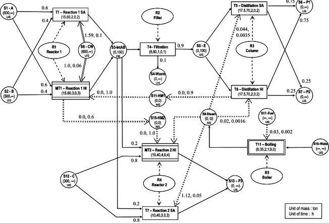
In order to demonstre the applicability of the proposed model, we consider a short-term scheduling problem that seeks to determine the optimal utilization of the available plant resources (processing equipment, storage capacity, utilities, etc) over a given time horizon. The multipurpose plant considered is an extension of a classical batch process example used by (Majozi, 2006) or (Chen et al, 2008). It consists of a plant manufacturing three products P1, P2 and P3 and production requirements are imposed on them at the end of the horizon. The generic recipe includes four operations (Reaction 1, Filtration, Distillation and Reaction 2) and the site recipe is described by the ERTN on Figure 3. Proportions of each material, minimum and maximum batch size, duration of tasks and storage capacity and policy are indicated. Moreover, the processing equipment available in the plant includes two pairs of units which are coupled to each other through a heat exchanger (Reactor 1/Column reboiler and Reactor 1/Reactor 2). Assuming appropriate temperature levels, there is in principle the opportunity of exchanging heat between, on the one hand, the exothermic Reaction 1 task which requires cooling and the Distillation task which requires heating and, on the other hand, the exothermic Reaction 1 task which requires cooling and the endothermic Reaction 2 task which requires heating. As mentionned in section 2, these operations have to be splitted in two tasks (SA:stand-alone or HI:heat integrated). The precise operating mode and heat characteristics of two heat-integrated processing steps taking place in a given pair of equipment items are known. The equipment is also fitted with exchange facilities that allow the use of external utilities (e.g., steam, cooling water) to supplement the heating and cooling loads provided through heat integration. The existence of these additional facilities also makes possible the use of each of the equipment items in a pair

for carrying out the corresponding processing step separately, if necessary, i.e. without the need for heat integration. In this context, the processing times of the individual steps when performed separately is different from those for the same steps when heat integration is employed (see Figure 3). In any case, the instantaneous rates of consumption of external utilities over the duration of each step are given on the ERTN (see Figure 3).

Figure 3. ERTN for example process

Concerning the pair Reaction 1/Distillation, the heat exchange match would involve task Reaction 1 being performed in the Reactor 1 and the Distillation task in the Column with an offset of 1 h with respect to their starting times. Indeed, such an offset is necessary in order to maximise the potential for heat integration by allowing sufficient time for the Reaction 1 to reach the operating temperature at which the heat consumed by the Distillation is to be generated. Due to the lower temperature differences, the duration of the Reaction 1 when operated in heat-integrated mode is increased from 2 to 3 hr. As expected, the demands posed by these tasks on external utilities are also modified. So, the macro-task MT1 is decomposed as shown in Figure 4.

Figure 4. Decomposition of the macro-task MT1

Similar remarks can be made about the pair Reaction 1/Reaction 2. The heat-integrated Reaction 1 task always requires a cooling water flow rate of 1.0 + 0.06B t/h during the first hour of its operation only ;

0.4 S1 - A (600,∞) UIS 0.4 0.6 0.6 0.25 S3-IntAB (0,100) FIS T5 – Distillation SA (17.5,70,2,0,2) T1 – Reaction 1 SA (15,60,2,0,2) R1 Reactor 1 T4– Filtration (8,80,1,0,1) S2 - B (500,∞) UIS S5 - E (0,100) UIS MT1 – Reaction 1 HI (15,60,3,0,3) S8 - CW (600,∞) UIS R2 Filter S4-Waste (0,∞) UIS S6 – P1 (0,∞) UIS S7 – P2 (0,∞) UIS T6 – Distillation HI (17.5,70,2,0,2) 0.25 0.75 0.75 R3 Column T7 – Reaction 2 SA (10,40,3,0,3) MT2 – Reaction 2 HI (10,40,4,0,4) S12 - C (300, ∞) UIS 0.2 0.2 0.8 0.8 R4 Reactor 2 S9-Steam (0, 0) NIS S13 – P3 (0, ∞) UIS S11-HM1 (0,0) NIS S15-HM2 (0,0) NIS 0.1 0.9 S16–Water (∞, ∞) UIS T11 – Boiling (0,35,2,1,0,0) R5 Boiler S17–Fuel (∞, ∞) UIS 1.59, 0.1 1.0, 0.06 0.0, 0.6 0.0, 0.9 0.044, 0.0035 0.02, 0.0016 0.03, 0.002

Unit of mass : ton Unit of time : h 1.12, 0.05 0.0, 1.0 0.0, 1.0 0.4 S1 - A (600,∞) UIS S1 - A (600,∞) UIS 0.4 0.6 0.6 0.25 S3-IntAB (0,100) FIS S3-IntAB (0,100) FIS T5 – Distillation SA (17.5,70,2,0,2) T5 – Distillation SA (17.5,70,2,0,2) T1 – Reaction 1 SA (15,60,2,0,2) R1 Reactor 1 R1 Reactor 1 T4– Filtration (8,80,1,0,1) T4– Filtration (8,80,1,0,1) S2 - B (500,∞) UIS S2 - B (500,∞) UIS S5 - E (0,100) UIS S5 - E (0,100) UIS MT1 – Reaction 1 HI (15,60,3,0,3) MT1 – Reaction 1 HI (15,60,3,0,3) S8 - CW (600,∞) UIS S8 - CW (600,∞) UIS R2 Filter R2 Filter S4-Waste (0,∞) UIS S6 – P1 (0,∞) UIS S6 – P1 (0,∞) UIS S7 – P2 (0,∞) UIS S7 – P2 (0,∞) UIS T6 – Distillation HI (17.5,70,2,0,2) T6 – Distillation HI (17.5,70,2,0,2) 0.25 0.75 0.75 R3 Column R3 Column T7 – Reaction 2 SA (10,40,3,0,3) T7 – Reaction 2 SA (10,40,3,0,3) MT2 – Reaction 2 HI (10,40,4,0,4) MT2 – Reaction 2 HI (10,40,4,0,4) S12 - C (300, ∞) UIS S12 - C (300, ∞) UIS 0.2 0.2 0.8 0.8 R4 Reactor 2 R4 Reactor 2 S9-Steam (0, 0) NIS S9-Steam (0, 0) NIS S13 – P3 (0, ∞) UIS S13 – P3 (0, ∞) UIS S11-HM1 (0,0) NIS S11-HM1 (0,0) NIS S15-HM2 (0,0) NIS S15-HM2 (0,0) NIS 0.1 0.9 S16–Water (∞, ∞) UIS S16–Water (∞, ∞) UIS T11 – Boiling (0,35,2,1,0,0) T11 – Boiling (0,35,2,1,0,0) R5 Boiler R5 Boiler S17–Fuel (∞, ∞) UIS S17–Fuel (∞, ∞) UIS 1.59, 0.1 1.0, 0.06 0.0, 0.6 0.0, 0.9 0.044, 0.0035 0.02, 0.0016 0.03, 0.002

Unit of mass : ton Unit of time : h 1.12, 0.05 0.0, 1.0 0.0, 1.0 0.4 S1 - A (600,∞) UIS 0.6 S3-IntAB (0,100) FIS R1 Reactor 1 S2 - B (500,∞) UIS MT1 – Reaction 1 HI (15,60,3,0,3) S8 - CW (600,∞) UIS S11-HM1 (0,0) NIS S15-HM2 (0,0) NIS 1.0, 0.06 0.0, 0.6 0.0, 1.0 0.4 S1 - A (600,∞) UIS 0.6 S2 - B (500,∞) UIS T2 – Reaction 1 HI1 (15,60,1,0,1) R1 Reactor 1 S3-IntAB (0,100) FIS 1.0, 0.06 S8 - CW (600,∞) UIS S15-HM2 (0,0) NIS 0.0, 0.6 S11-HM1 (0,0) NIS 0.0, 1.0 S10-Int1 (0,0) NIS T3 – Reaction 1 HI2 (15,60,2,0,2) T10 – Reaction 1 HI3 (15,60,2,0,2) 0.4 S1 - A (600,∞) UIS 0.6 S3-IntAB (0,100) FIS R1 Reactor 1 S2 - B (500,∞) UIS MT1 – Reaction 1 HI (15,60,3,0,3) S8 - CW (600,∞) UIS S11-HM1 (0,0) NIS S15-HM2 (0,0) NIS 1.0, 0.06 0.0, 0.6 0.0, 1.0 0.4 S1 - A (600,∞) UIS S1 - A (600,∞) UIS 0.6 S3-IntAB (0,100) FIS S3-IntAB (0,100) FIS R1 Reactor 1 R1 Reactor 1 S2 - B (500,∞) UIS S2 - B (500,∞) UIS MT1 – Reaction 1 HI (15,60,3,0,3) MT1 – Reaction 1 HI (15,60,3,0,3) S8 - CW (600,∞) UIS S8 - CW (600,∞) UIS S11-HM1 (0,0) NIS S11-HM1 (0,0) NIS S15-HM2 (0,0) NIS S15-HM2 (0,0) NIS 1.0, 0.06 0.0, 0.6 0.0, 1.0 0.4 S1 - A (600,∞) UIS 0.6 S2 - B (500,∞) UIS T2 – Reaction 1 HI1 (15,60,1,0,1) R1 Reactor 1 S3-IntAB (0,100) FIS 1.0, 0.06 S8 - CW (600,∞) UIS S15-HM2 (0,0) NIS 0.0, 0.6 S11-HM1 (0,0) NIS 0.0, 1.0 S10-Int1 (0,0) NIS T3 – Reaction 1 HI2 (15,60,2,0,2) T10 – Reaction 1 HI3 (15,60,2,0,2) 0.4 S1 - A (600,∞) UIS S1 - A (600,∞) UIS 0.6 S2 - B (500,∞) UIS S2 - B (500,∞) UIS T2 – Reaction 1 HI1 (15,60,1,0,1) T2 – Reaction 1 HI1 (15,60,1,0,1) R1 Reactor 1 R1 Reactor 1 S3-IntAB (0,100) FIS S3-IntAB (0,100) FIS 1.0, 0.06 S8 - CW (600,∞) UIS S8 - CW (600,∞) UIS S15-HM2 (0,0) NIS S15-HM2 (0,0) NIS 0.0, 0.6 S11-HM1 (0,0) NIS S11-HM1 (0,0) NIS 0.0, 1.0 S10-Int1 (0,0) NIS S10-Int1 (0,0) NIS S10-Int1 (0,0) NIS T3 – Reaction 1 HI2 (15,60,2,0,2) T3 – Reaction 1 HI2 (15,60,2,0,2) T10 – Reaction 1 HI3 (15,60,2,0,2) T10 – Reaction 1 HI3 (15,60,2,0,2)

Axx-6

thereafter all its needs are satisfied through heat exchange with the contents of the Reactor 2. On the other hand, the heat-integrated Reaction 2 task requires a constant steam flow rate of 0.9+0.031B t/h during the first two hours (task T8) and a constant steam flow rate of 0.3+0.006B t/h thereafter (task T9), supplementing the energy received from the heat exchange with the Reactor 1 contents.

Finally, unlimited availability cooling water is assumed. In contrast, steam flow rate is limited and produced by a site utility system (boiling operation T11 that consumes fuel).

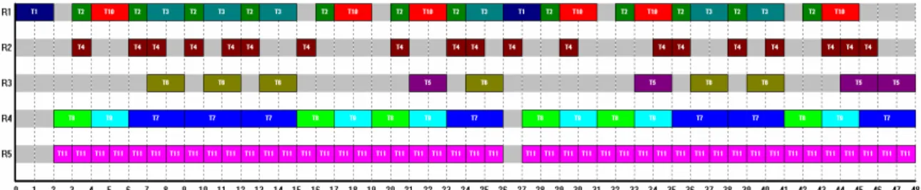
Figure 5. Scheduling corresponding to the manufacturing of 510 t of P1, 170 t of P2 and 300 t of P3

Figure 5 shows the optimal schedule obtained for this problem (solve on a 2.0 GHz Pentium with XPRESS-MP) on a time horizon of 48h. The number inside each rectangle in the Gantt chart denotes the task being carried out. It can be seen that this involves both stand-alone operations and integrated ones. Stand-alone tasks are performed sporadically throughout the horizon. This feature of the optimal solution is due to the complex trade-off between increased processing time and reduced utility consumption for the two reaction tasks. Moreover, as expected, heat integrated Reaction 1 takes place as soon it is possible in order to reduce the consumption of steam of the other integrated operations. Finally, the costs of the utilities consumed are reduced to an even larger extent.

5. Conclusion

This paper has proposed a systematic mathematical framework for the exploitation of heat integration in multipurpose batch plant operation, taking detailed account of its interactions with production scheduling. The ERTN formalism has been used to model clearly and unambiguously both the material and utilities flows in the dicontinuous process. Based on this representation, a general scheduling formulation including direct heat integration aspects was examined and an example illustrates the potentiel benefits of this approach. Currently, a continuous time MILP formulation and indirect heat integration are under consideration.

Références

Agha M., 2009. Integrated management of energy and production : scheduling of batch processes and CHP plants, Thèse de Doctorat, INP de Toulouse, France,

Burkard R.E. et Hatzl J., 2005, Review, extensions and computational comparison of MILP formulations for scheduling of batch processes, Computers and Chemical Engineering, 29, 1752-1769

Chen C.L., Chang C.Y., 2008, A resource-task network approach for optimal short-term /periodic scheduling and heat integration in multipurpose batch plants, Applied Thermal Engineering

Fabre, F., Hétreux, G., Le Lann J.M., Zaraté, P., 2011, Dynamic hybrid simulation of batch processes driven by a

scheduling module. Computers and Chemical Engineering, doi:10.1016/j.compchemeng.2011.04.007

Floudas C.A. et Lin X., 2004, Continuous-time versus discrete-time approaches for scheduling of chemical processes : a review, Computers and Chemical Engineering, 28, 2109-2129

Méndez C.A., Cerdá J., Grossmann I.E., Harjunkoski I. et Fahl M., 2006, State-of-the-art review of optimization methods for short-term scheduling of batch processes, Computers and Chemical Engineering, 30, 6-7, 913-946 Linnhoff, B., Ashton, G.J., Obeng, E.D.A, 1988, Process Integration of Batch Processes, Inst. Chem. Eng. Symp.

Serr., 109, 221-237

Majozi T., 2006, Heat integration of multipurpose batch plants using a continuous-time framework, Applied Thermal Engineering, 26, 1369-1377

Pantelides C.C., 1994, Unified Framework For The Optimal Process Planning And Scheduling, CACHE Publications. Proceedings of the Second Conference on Foundations of Computer Aided Operations, p. 253-274.

Thery R., Hétreux G., AghaM.H., Haït, _{A., Le LannJ.M., 2011, The Extended Resource Task Network: a framework}