What drives the observed variability of HCN in the troposphere and lower stratosphere?

(1)

Chemistry

and Physics

What drives the observed variability of HCN in the troposphere and

lower stratosphere?

Q. Li1, P. I. Palmer1, H. C. Pumphrey1, P. Bernath2, and E. Mahieu3

1_{School of GeoSciences, The University of Edinburgh, Edinburgh, UK} 2_{Department of Chemistry, University of York, York, UK}

3_{Institute of Astrophysics and Geophysics, University of Li`ege, Li`ege, Belgium}

Received: 7 April 2009 – Published in Atmos. Chem. Phys. Discuss.: 4 May 2009

Revised: 26 September 2009 – Accepted: 28 September 2009 – Published: 10 November 2009

Abstract. We use the GEOS-Chem global 3-D chemistry transport model to investigate the relative importance of chemical and physical processes that determine observed variability of hydrogen cyanide (HCN) in the troposphere and lower stratosphere. Consequently, we reconcile ground-based FTIR column measurements of HCN, which show annual and semi-annual variations, with recent space-borne measurements of HCN mixing ratio in the tropical lower stratosphere, which show a large two-year variation. We find that the observed column variability over the ground-based stations is determined by a superposition of HCN from sev-eral regional burning sources, with GEOS-Chem reproduc-ing these column data with a positive bias of 5%. GEOS-Chem reproduces the observed HCN mixing ratio from the Microwave Limb Sounder and the Atmospheric Chemistry Experiment satellite instruments with a mean negative bias of 20%, and the observed HCN variability with a mean negative bias of 7%. We show that tropical biomass burning emissions explain most of the observed HCN variations in the upper troposphere and lower stratosphere (UTLS), with the remain-der due to atmospheric transport and HCN chemistry. In the mid and upper stratosphere, atmospheric dynamics progres-sively exerts more influence on HCN variations. The extent of temporal overlap between African and other continental burning seasons is key in establishing the apparent bienniel cycle in the UTLS. Similar analysis of other, shorter-lived trace gases have not observed the transition between annual and bienniel cycles in the UTLS probably because the sig-nal of inter-annual variations from surface emission has been diluted before arriving at the lower stratosphere (LS), due to shorter atmospheric lifetimes.

Correspondence to: Q. Li

(q.li@ed.ac.uk)

1 Introduction

Hydrogen cyanide (HCN) is a tracer of biomass burning (BB; Lobert et al., 1990; Holzinger et al., 1999) and could play a non-negligible role in the nitrogen cycle (Li et al., 2000, 2003). Before we can confidently use HCN to infer its sur-face sources and sinks we must first develop a robust under-standing of the chemical and physical processes that deter-mine observed variability.

Laboratory and field measurements support that BB is the major source for atmospheric HCN but the magnitude is still uncertain (0.1–3.2 Tg N/year) (Li et al., 2003 and references therein). Automobile exhaust and industrial processes repre-sent additional minor tropospheric sources of HCN (Lobert et al., 1991; Bange and Williams, 2000; Holzinger et al., 2001). The HCN source from burning domestic biofuel is still unclear with studies reporting values from zero, based on laboratory fire measurements in Africa (Bertschi et al., 2003), to 0.2 Tg N/year based on analysis of aircraft con-centration measurements over the western Pacific downwind of eastern Asia (Li et al., 2003), the range probably reflect-ing regional differences in the nitrogen content of domes-tic biofuels. Ocean uptake has been hypothesized as the dominant tropospheric sink with values ranging from 0.73 to 1.0 Tg N/year, where it is biologically consumed (Singh et al., 2003), leading to a lifetime of 5 months in the tropo-sphere (Hamm and Warneck, 1990; Li et al., 2003). Addi-tional minor sinks of HCN include atmospheric oxidation by the hydroxyl radical (OH) and O(1D), photolysis, yielding a stratospheric lifetime of a few years (Cicerone and Zellner, 1983; Brasseur et al., 1985). Li et al. (2000, 2003) showed using the GEOS-Chem global 3-D model that the observed seasonal variation of the HCN tropospheric column in differ-ent regions of the world was consistdiffer-ent with a scenario where BB provides the main source and ocean uptake provides the

(2)

main sink. Recently Lupu et al. (2009) reproduced similar seasonal variations of the HCN tropospheric column using the GEM-AQ tropospheric global 3-D model.

Ground-based HCN column measurements from Fourier transform infrared (FTIR) spectrometers, available at several sites around the world (Mahieu et al., 1995, 1997; Rinsland et al., 1999, 2000, 2001, 2007; Zhao et al., 2000, 2002), represent important but sparse constraints to our quantitative understanding of HCN spatial and temporal distributions. As we show later these data show large variations on intra-seasonal to yearly timescales. Recent analysis of satellite HCN measurements from the NASA Aura Microwave Limb Sounder (MLS) (Waters, 2006) and the Atmospheric Chem-istry Experiment Fourier Transform Spectrometer (ACE-FTS) (Boone et al., 2005) show an approximate 2-year cy-cle of HCN anomalies in the tropical upper troposphere and lower stratosphere (UTLS) (Pumphrey et al., 2008), hypoth-esized to be due to year-to-year variations in surface burn-ing over Indonesia and Australia. This is supported by a recent model study of year-to-year variations of UTLS CO, another tracer of BB, which showed that variations during 1994–1998 were primarily caused by year-to-year changes in surface burning (Duncan et al., 2007). The satellite mea-surements of HCN from MLS and ACE-FTS therefore po-tentially provide additional global constraints on BB emis-sions but first we have to reconcile the observed annual cycle from ground-based and 2-year cycle from MLS and ACE-FTS measurements. We use the GEOS-Chem global 3-D chemical transport model (CTM) (Bey et al., 2001; Li et al., 2003) to understand the role of surface emissions, and atmo-spheric chemistry and transport in determining the observed variations of HCN from ground-based and space-borne mea-surements.

In the next section we describe the GEOS-Chem HCN simulation and evaluate model concentrations using ground-based FTIR and space-borne measurements. In Sect. 3 we examine the model ability to reproduce observed tropical HCN anomalies and in Sect. 4 we determine the importance of surface biomass burning emissions, atmospheric chem-istry and transport in reproducing this tropical signal. We conclude the paper in Sect. 5.

2 Description and evaluation of GEOS-Chem HCN simulation

2.1 Model description

We use the GEOS-Chem global 3-D CTM (version 7.4.11) to simulate the atmospheric distribution of HCN from 2001 to 2008. Our calculations use assimilated meteorological analy-ses from the Goddard Earth Observing System v4 (GEOS-4, available from 1990 to 2006, used here from 2001 to 2003) and v5 (GEOS-5, available from 2003 to present, used here from 2004 to 2008) of the NASA GMAO (Global

Model-ing and Assimilation Office), at 6-h temporal resolution (3-h for surface variables and mixed layer depths). We use the model with a horizontal resolution of 2◦_×_2.5◦_{(Lat. ×Lon.)} and with 30 levels in 2001–2003 (derived from the native 55 levels of GEOS-4) ranging from the surface to the meso-sphere, 20 of which are below 12 km. In 2004–2008, we run the model with the horizontal resolution of 2◦×2.5◦and with 47 levels (derived from the native 72 levels of GEOS-5) with same levels in the stratosphere and 17 more levels in the troposphere, using a re-gridded restart file from the earlier experiment of 2001–2003. The model outputs are interpo-lated onto the same levels. Here we focus on model details pertinent to the HCN simulation; for a more detailed descrip-tion of the GEOS-Chem model we refer the reader to Bey et al. (2001) and Fiore et al. (2003).

The HCN simulations are conducted for a 8-year pe-riod (January 2001–December 2008), using the previous 24 months to remove initial conditions. Correspondingly, we study the ground-based observation from January 2001 to December 2008, and space-borne observations of ACE-FTS (available from January 2004 to August 2007) and Aura MLS (available from September 2004 to December 2008). The time domain of our analysis is limited by the availabil-ity of BB emissions data (see below). We use fixed 3-D monthly mean OH fields, (described below), that linearize the HCN simulation, allowing us to describe total HCN con-centrations as a linear sum of contributions from individual source regions/types. We assume no inter-annual variability of OH concentrations. For our experiments, we include two continental sources: BB and domestic biofuel burning. Fig-ure 1 shows the ten source regions we study in this paper: North America (NA), South America (SA), Europe (EU), northern Africa (NAF), Southern Africa (SAF), Boreal Asia (BA), Southeast Asia (SE AS), and Indonesia and Australia (IND + AUS); Table 1 defines the latitude and longitude do-main of each geographical region.

We use monthly mean BB emission estimate of HCN, based on CO estimates from the Global Fire Emission Database version 2 (GFEDv2, available from 1997 to 2008; van der Werf et al., 2006), using an observed HCN:CO emis-sion ratio of 0.27% over the western Pacific (Li et al., 2003). Figure 2 shows that global HCN BB emissions peak in August and to a lesser extent in January, with global an-nual mean values ranging from 0.56 to 0.77 Tg N/year over 2001–2008. The largest emissions originate from Africa, SA, IND + AUS, SE AS and BA, with only small emissions from NA and EU. Figure 2 also shows that the zonal mean of BB over 2001–2008 is generally larger in the tropics, as expected, with northern tropical regions (NAF) leading the southern tropics (SAF, SA) by approximately 8 months. Monthly mean emissions of domestic biofuel burning have a small seasonal cycle related to the heating source and are based on CO emission estimates from Streets et al. (2003), scaled by an HCN emission factor of 1.6% (Li et al., 2003). We estimate a global domestic biofuel burning HCN source

(3)

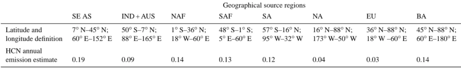
Table 1. Geographical definitions of source regions and associated HCN annual flux estimates (Tg N/year)

over 2001–2008 (biomass burning + domestic biofuel burning).

Geographical source regions

SE AS IND + AUS NAF SAF SA NA EU BA

Latitude and 7◦N–45◦N; 50◦S–7◦N; 1◦S–36◦N; 48◦S–1◦S; 57◦S–16◦N; 16◦N–88◦N; 36◦N–88◦N; 45◦N–88◦N; longitude definition 60◦E–152◦E 88◦E–165◦E 18◦W–60◦E 5◦E–60◦E 95◦W–32◦W 173◦W–50◦W 18◦W –60◦E 60◦E–180◦E HCN annual

emission estimate 0.19 0.09 0.14 0.13 0.12 0.04 0.03 0.14

Fig. 1. Geographical source regions for the linearly decomposed

HCN simulation. The regions are denoted North America (NA), South America (SA), Europe (EU), Boreal Asia (BA), North Africa (NAF), Southern Africa (SAF), Southeast Asia (SE AS), and In-donesia and Australia (IND + AUS). See Table 1 for latitude and longitude definitions and associated flux estimates.

of 0.22 Tg N/year, with the largest contributions from Asia (0.19 Tg N/year) and EU (0.02 Tg N/year). Table 1 shows the estimates of HCN emission over 2001–2008 (BB + domestic biofuel burning) from each region. Emissions over the study regions are comparable in magnitude, except over NA and EU, where they are an order of magnitude smaller (<50% of others); we do not investigate further NA and EU. We in-clude the ocean uptake of HCN by air-to-sea HCN transfer flux, following Li et al. (2003). We estimate an ocean sink of 0.73 Tg N/year, peaking in September-December due to the higher surface sea temperature (SST) in the southern hemi-sphere, reflecting the correlation between HCN deposition velocity over oceans and SST (Singh et al., 2003; Li et al., 2000, 2003).

The largest atmospheric sink of HCN is due to chemical reaction with OH. We use monthly mean tropospheric OH fields from a full-chemistry GEOS-Chem (version 5.07.08) simulation, and use monthly mean stratospheric OH fields from Aura MLS v2.2 data from September 2004 to Decem-ber 2008, distinguishing between day/night (for each cal-endar month, fields were produced for day time and night time, respectively) values (Pickett et al., 2006, 2008). The HCN + OH reaction rate coefficient is taken from recent

anal-(a)

(b)

Fig. 2. Seasonal variation of global and regional mean of biomass

burning sources and the ocean sink of HCN (Tg N/month) over 2001–2008. Vertical lines denote the ±1-standard deviation about the mean value. Biomass burning emissions are based on GFEDv2 (van der Werf et al., 2006) and scaled by using an observed HCN:CO emission ratio of 0.27% (Li et al., 2003). The ocean sink parameterization follows Li et al. (2003). (a) Global emissions and ocean uptake; (b) emissions from individual regions.

ysis (Kleinboehl et al., 2006) that recommends using a value that is 40% smaller than values used in previous modelling studies (Li et al., 2003). This HCN sink represents a loss of approximately 0.12 Tg N/year. The sink of HCN due to reac-tion with O(1D), the rate constant taken from Kleinboehl et al. (2006), represents a minor sink for HCN and we do not discuss this further. We also include a source of HCN from the oxidation of CH3CN by OH, using a 30% molar yield

(4)

(Kleinboehl et al., 2006). We acknowledge this molar yield is extremely uncertain and in Sect. 4.2 we present a sensitiv-ity calculation that does not include this HCN source.

2.2 Model evaluation

2.2.1 Ground-based FTIR observations

Ground-based FTIR observations of HCN vertical columns are available at Mauna Loa, Hawaii (19.5◦N, 155.6◦W, al-titude 3.4 km), Kitt Peak, Arizona (31.9◦N, 116◦W, altitude 2.09 km), and the Jungfraujoch research station, Switzerland (46.6◦_{N, 8.0}◦_{E, altitude 3.58 km), from the Network for} Detection of Atmospheric Composition Change (NDACC, http://www.ndacc.org). GEOS-Chem is sampled at the lo-cation of each station and convolved with the instrument-specific averaging kernel (Mahieu et al., 1995, 1997; Rins-land et al., 1999, 2000, 2001, 2007).

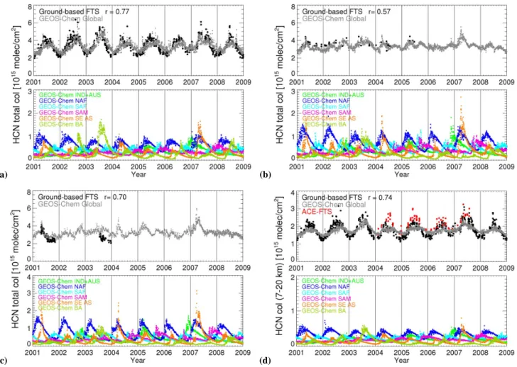
Figure 3 shows the observed and model HCN total columns at the three stations between 2001 and 2008. In general, we find reasonable agreement (typical bias less than 10%) between the model and observed HCN columns, ac-knowledging that at some stations the measurement cover-age is sparse. Observed and model total columns of HCN at Jungfraujoch show a strong seasonal cycle with peaks during mid-summer and troughs during mid-winter, with model bias typically within +3%. Using our linearly decomposed HCN simulation over Jungfraujoch we show that the seasonal cy-cle is determined by NAF and BA BB. In particular, the large 2002 and 2003 fire seasons (van der Werf et al., 2006) over BA are captured at this location. At the lower latitude sta-tions, Mauna Loa and Kitt Peak, the seasonal cycle is less pronounced due to the superposition of many regional burn-ing signatures. Model bias is typically less than +5% but can reach +25% (e.g., Summer/Autumn 2003 over Mauna Loa). Model HCN columns over Mauna Loa and Kitt Peak have a strong intraseasonal variation, peaking in March and September. Early in the calendar year, total HCN column variations are determined by NAF, SE AS and IND + AUS. Southern hemisphere burning peaks over SAF and SA dur-ing September–October. Elevated burndur-ing durdur-ing 2001 over SE AS is captured by the model and measurements over Mauna Loa.

Figure 3 also shows partial (7–20 km) HCN vertical columns over Jungfraujoch, which exhibit a similar but weaker seasonal cycle evident in the total columns. The model captures the broad seasonal cycle of HCN over this altitude range (discrepancies are typically less than 1%), but cannot capture observed values at the peaks and troughs. Space-borne HCN data from the ACE-FTS satellite instru-ment (Boone et al., 2005) provides additional information over Jungfraujoch. ACE is a Canadian-led solar occulta-tion mission launched in August 2003 into a circular orbit inclined at 74◦ to the Equator (Bernath et al., 2005), mea-suring up to 30 occultations per day that mainly sample

mid-and high-latitudes. The vertical resolution of ACE-FTS is 3 to 4 km, limited by the instrument field of view. We use the ACE-FTS version 2 volume mixing ratio (vmr) profiles which aare currently available from January 2004 to Au-gust 2007. Compared to ground-based FTIR spectrometers, the ACE-FTS instrument has a lower frequency of obser-vation at any given ground station (it crosses the Equator 8 times per year). We use the latitudinal average of ACE-FTS data that fall within 41–51◦N. The interannual varia-tions of ACE-FTS HCN are in a good qualitative agreement with the ground-based measurements but still with a positive bias of 17%. The model generally reproduces the ground-based observations with a positive bias of 5%. Our evaluation of the model is limited due to the lack of available ground-based data.

2.2.2 Space-borne observations

Satellite measurements have the major advantage of ob-taining global coverage and therefore putting observed HCN variations at fixed stations into a broader context. For our study we use HCN retrievals from the ACE-FTS in-strument (described above) and the Aura Microwave Limb Sounder (MLS). The MLS instrument (Waters, 2006) was launched in July 2004 aboard the Aura spacecraft. MLS is an emission limb sounder, operating in the millimetre and sub-millimetre spectral regions. A single day of observa-tions consists of 3495 scans across the Earth’s limb and cov-ers all latitudes between 82◦_{S and 82}◦_{N with a resolution} of about 1.5◦_{of latitude. Successive orbits are separated by} 25◦ of longitude. MLS makes daily, global measurements of 14 trace species using 32 spectrometers distributed across five different regions of the spectrum. The HCN mixing ratio is retrieved from a spectrometer centred on the 177.26 GHz spectral line. Further details can be found in Pumphrey et al. (2006, 2008), who note that the standard version 2.2 daily HCN product is noisy and has large biases in the lower strato-sphere, especially in the high latitudes due to the interference of HNO3. As a result, an alternative HCN product was

devel-oped which has reduced noise at the cost of being available as a weekly zonal mean (Pumphrey, 2006, 2008). In this study, we use the weekly zonal mean HCN data to validate the model HCN mixing ratio.

Figure 4 shows zonal mean of ACE-FTS HCN concen-tration from September 2004 to August 2007 and the global 3-D model fields sampled at the time and location of ACE-FTS data, taking into account the ACE-ACE-FTS field-of-view. The model only captures the broad features of the zonal mean distribution and generally has a negative bias (typi-cally ∼15%) in the UTLS compared with ACE-FTS. This bias is consistent with our previous comparison with ground-based FTS data that showed ACE-FTS data had a positive bias of 17% relative to ground-based column data. Figure 4 shows the model is better at capturing observed HCN tempo-ral standard deviations (σ ), with a typical value of ∼10 pptv

(5)

(a) (b)

(c) (d)

Fig. 3. Time series of FTS-observed (black dots) and GEOS-Chem model (grey dots) HCN total columns (1015molec/cm2) over (a) Jungfraujoch, Switzerland (46.6◦N, 8.0◦E, altitude 3.58 km); (b) Kitt Peak, Arizona (31.9◦N, 116◦W, altitude 2.09 km); and (c) Mauna Loa, Hawaii (19.5◦N, 155.6◦W, altitude 3.4 km). (d) shows observed and model HCN columns between 7 km and 20 km over Jungfraujoch station, with the red dots denote the latitudinal average of HCN columns measured by the ACE-FTS satellite instrument falling within 41◦N–51◦N. Other colors denote HCN contributions from regional BB emissions. Vertical lines denote calendar years. The correlation coefficient r denotes the correlation between measurements of HCN columns and model HCN columns; correlations>0.1 over Jungfraujoch, and correlations>0.2 over Kitt Peak and Mauna Loa, are statistically significant to the 99% confidence level.

in tropical UTLS. GEOS-Chem shows a stronger hemispher-ical asymmetry in the upper troposphere than ACE-FTS, sug-gesting an overestimate of emissions in northern hemisphere in the model. Both ACE-FTS and GEOS-Chem HCN show a low HCN mixing ratio in southern mid-high latitudes, imply-ing a large ocean sink of HCN (Li et al., 2000, 2003). Fig-ure 4 also shows model and MLS weekly zonal mean of HCN from September 2004 to December 2008. MLS measure-ments show a similar HCN distribution as ACE-FTS mea-surements show, with high mixing ratios in tropical UTLS and lower mixing ratios in mid and high latitudes. The model reproduces only the broad features of the zonal mean distri-bution observed by MLS, and has a larger negative bias (typ-ically ∼25%) in the tropical UTLS. As we show below, of more importance in this study is the ability of the model to accurately simulate the temporal variations of HCN in the UTLS as observed by MLS and ACE-FTS.

3 Model and observed variability of HCN in the troposphere and stratosphere

Atmospheric transport from the troposphere to the strato-sphere generally plays an important role in the atmospheric distribution of trace gases. Over the tropics, deep convection via cumulonimbus clouds reaching the UTLS and large-scale ascent via the major upward branch of the Brewer-Dobson (BD) circulation in the stratosphere represent the dominant vertical transport processes. For trace gases over the tropics with an atmospheric lifetime longer than the transit time from the tropopause to the mid-stratosphere, a clear upward trans-port of the signal of seasonal cycle is called the “atmospheric tape recorder” (Mote et al., 1996). For H2O, there is a clear

annual tape recorder effect (Mote et al., 1996) in the tropi-cal UTLS. For CO, the annual tape recorder is also observed below 20 km (Schoeberl et al., 2006). However, a recent

(6)

(a) (b)

(c) (d)

(e) (f)

(g) (h)

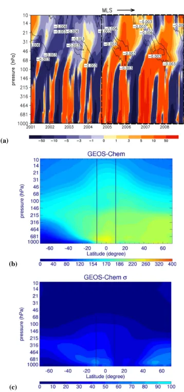
Fig. 4. GEOS-Chem model and observed zonal mean distributions of HCN (pptv) and associated standard deviations (pptv) as a function of

pressure (hPa). The GEOSChem model, run at 2◦×2.5◦horizontal resolution, is sampled at the time and location of each observed scene.

(a) and (b) show zonal mean HCN distributions from the Atmospheric Chemistry Experiment (ACE) and the GEOS-Chem model from 1

September 2004 to 31 August 2007; and (c) and (d) show the corresponding standard deviations from those mean values. (e) and (f) show zonal mean HCN distributions from the Microwave Limb Sounder (MLS) and from GEOS-Chem from 1 September 2004 to 31 December 2008; and (g) and (h) show the corresponinding standard deviations from those mean values. We use weekly zonal mean MLS products (Pumphrey et al., 2008). The two vertical lines define the tropical region (10◦S–10◦N) over which the HCN anomalies are calculated.

(7)

analysis of HCN anomalies from Aura MLS and ACE-FTS instruments showed an approximate 2-year cycle (Pumphrey et al., 2008), and it was suggested that this was partly due to the year-to-year variability in BB emissions over Indonesia and Australia.

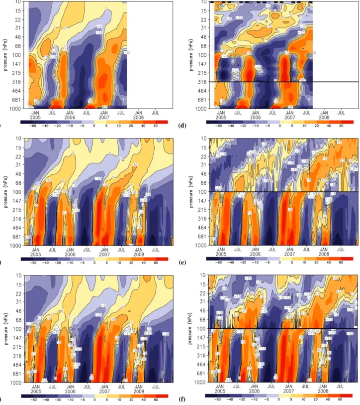
We determine HCN anomalies, defined here as the fluc-tuation from the time mean, from ACE-FTS and MLS data and the GEOS-Chem model. Model HCN anomalies are cal-cuated by sampling the model in the same way as MLS and ACE-FTS sample the real atmosphere. Figure 5 shows that model HCN anomalies in the troposphere alternate between positive and negative on a 12-month cycle, with the positive anomalies occurring from September to January and negative anomalies from February to August. These positive anoma-lies correspond to the peaks of BB emissions from tropical regions of IND + AUS, SA and NAF in September to Jan-uary as shown in Fig. 2. Figure 5 shows that there is remark-able agreement at the UTLS between model HCN anomalies in the troposphere and MLS and ACE-FTS HCN anomalies in the UTLS (with a typical bias of only 3%). This sug-gests that the model and measured HCN anomalies are con-sistent, and using the GEOS-Chem model as an intermedi-ary implies that the ground-based FTS data are consistent with MLS and ACE-FTS. However, the contour lines for the GEOS-Chem HCN slope upwards more steeply than those for the observed mixing ratios, implying that vertical trans-port in the model is faster than in the real atmosphere, partic-ularly at altitudes above 30 hPa (Figs. 10 and 11 of Schoe-berl et al., 2008). Due to the limited time resolution of ACE-FTS instrument, we smooth the ACE-FTS data in time to retrieve the continuous tape recorder of HCN. We use a kernel smoothing technique (Wand and Jones, 1995) with a bandwidth of 0.2 years. Consequently, seasonal variations of HCN in the troposphere (peaks in February/September and troughs in June/November), and similar stratospheric varia-tions but with a month lag, observed by MLS are not well captured by ACE-FTS. The 2-year cycle in the lower strato-sphere is still reproduced by the smoothed ACE data.

Figure 5 also shows the tape recorder of HCN retrieved from the MLS standard version 2.2 daily products. Although as we indicated in last section the zonal mean values of MLS standard daily HCN concentration products are generally not recommended for use in the lower stratosphere (Pumphrey et al., 2008), we find that HCN anomalies of MLS standard products agree with MLS weekly zonal mean products over the equatorial regions. We restrict our analysis to equato-rial regions where the interferences of HCN due to HNO3is

small.

We conducted the HCN simulation for a 8-year period (January 2001–December 2008), allowing us to put the relatively short ACE (used from September 2004 to Au-gust 2007) and MLS (used from September 2004 to De-cember 2008) record into a broader temporal perspective. Figure 6 shows that our results over the ACE-FTS and Aura MLS time period are consistent with the 8-year model

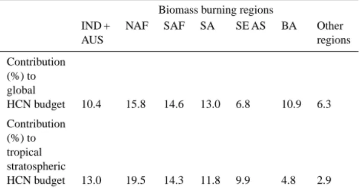
Table 2. The 2001–2008 mean percentage contribution of regional

biomass burning emissions to the global and stratosphere HCN bud-gets.

Biomass burning regions

IND + NAF SAF SA SE AS BA Other

AUS regions Contribution (%) to global HCN budget 10.4 15.8 14.6 13.0 6.8 10.9 6.3 Contribution (%) to tropical stratospheric HCN budget 13.0 19.5 14.3 11.8 9.9 4.8 2.9

calculation that encompasses approximately four 2-year cy-cles in the LS. Recent analysis of variability of MLS HCN measurements suggested the variations of surface burning in Indonesia and Australia might contribute to the 2-year vari-ations of HCN in the LS (Pumphrey et al., 2008). It has not escaped our attention that other sources of atmospheric vari-ability in the tropical UTLS (e.g., Quasi-Biennial Oscillation, the QBO, shown in Fig. 6) may also play a role in determin-ing the 2-year cycle. In the next section we investigate the role of atmospheric dynamics and regional BB emisions on determining the tropical variation of HCN through a sensi-tivity analysis of the model results.

Table 2 shows the 2001–2008 mean percentage contri-bution of regional BB emissions to the global HCN bud-get and to the tropical stratospheric HCN budbud-get. We find the largest contributions to the global budget are from IND + AUS, NAF, SAF, SA, and BA, all representing more than 10%. The largest stratospheric contributions are from IND + AUS, NAF, SAF, and SA, again all representing more than 10%. We find the increased stratospheric percentage contributions from individual HCN budget terms compared to the global values are from IND + AUS, NAF and SE AS, corresponding to the active tropical convective regions (Liu et al., 2005). BB emissions represent approximately 80% of tropical stratospheric HCN, with the remainder from domes-tic biofuel and from the oxidation of CH3CN (Sect. 2).

4 Sensitivity of results to biomass burning, dynamics and atmospheric chemistry

In this section we investigate how sensitive model HCN anomalies are to changes in our assumptions about at-mospheric dynamics, biomass burning and atat-mospheric chemistry.

(8)

(a) (d)

(b) (e)

(c) (f)

Fig. 5. GEOS-Chem model and observed HCN (pptv) tropical anomalies (10◦S–10◦N) as a function of pressure (hPa). The GEOS-Chem model, run at 2◦×2.5◦horizontal resolution, is sampled at the time and location of each observed scene. Model HCN anomalies as observed by (a) ACE-FTS, (b) MLS weekly zonal mean products (Pumphrey et al., 2008), and (c) MLS version 2.2 standard daily products. Model HCN anomalies (pptv) as observed by (d) ACE-FTS with observed anomalies superimposed from 316 hPa–10 hPa, (e) MLS weekly zonal mean with observed anomalies superimposed from 100 hPa–10 hPa, and (f) MLS standard daily mean with observed anomalies superimposed from 100 hPa–10 hPa. Circles in (d) indicate the times at which ACE-FTS makes measurements within 10◦S–10◦N.

(9)

4.1 Role of atmospheric dynamics and biomass burning sources

Figure 6 showed that the tape recorder effect of model HCN between 2001 and 2008 encompassed approximately four 2-year cycles in the lower stratosphere. To isolate the influ-ence of dynamics and BB emissions on variations in HCN, we calculate HCN anomalies using a single year of meteo-rology (2006 in this study) or BB emissions (2001 in this study), respectively, eliminating the effect of year-to-year variations in atmospheric transport or BB emissions, respec-tively. Figure 7 shows highest correlations between BB emissions and variability of HCN over the tropical tropo-sphere and lower/mid-tropotropo-sphere, suggesting that surface BB emissions are the primary driving factor for observed HCN variability in the troposphere and lower stratosphere. Surface emissions from Africa, Indonesia and Australia con-tribute the most to both the magnitude (Table 2) and variabil-ity of HCN over this vertical region. Figure 7 shows the year to year changes in meteorology (e.g., QBO) play a larger role in determining HCN variability in the upper stratosphere. Further investigation is required but this is outside the scope of this study.

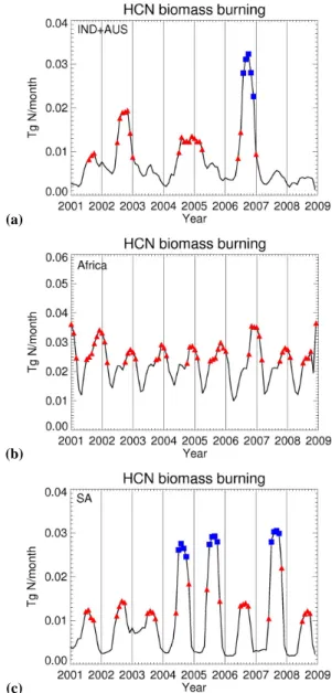
So why during some years is HCN anomalously high in the lower stratosphere? Figure 8 suggests that both the mag-nitude of the emissions and the length of burning seasons play a role. Here, we have identified monthly emissions that are greater than the 2001–2008 mean (denoted by red trian-gles) as a crude measure of peak burning months that de-termine the burning season; anomalous burning months (de-noted by blue squares) are 2.5 times greater than the mean. The African burning season, according to GFEDv2 estimates (van der Werf et al., 2006), is more regular in magnitude (peaking in late/early months) and timing than burning sea-sons from other continents, reflected in the contribution of atmospheric HCN from Africa BB emissions. Based on the small number of complete burning seasons, the only two common characteristics for anomalous high HCN concen-trations in the UTLS (2002/2003, 2004/2005, 2005/2006, 2006/2007, 2007/2008) is 1) larger than normal emissions and 2) longer burning seasons from IND + AUS and/or SA. We acknowledge that the duration of the burning season and the magnitude of emissions may be interrelated. During 2002/2003 and 2006/2007, BB emissions over IND + AUS are particularly high (Fig. 8), resulting in anomalously high contributions to atmospheric HCN in late 2002 and late 2006 (Fig. 7), that begin to overlap in time with lofted African airmasses. During 2004/2005, the burning season over IND + AUS was longer than normal (Fig. 8) and BB emis-sions over SA were anomalously large (Fig. 8). This resulted in anomalously high HCN contributions from both regions, overlapping in time with lofted African airmasses. During 2005/2006 and 2007/2008, anomalously high BB emissions from SA (Fig. 8) provide similar contributions to the HCN

(a)

(b)

(c)

Fig. 6. (a) GEOS-Chem model tropical (10◦S–10◦N) HCN anomalies (pptv) between 2001 and 2008. Contours denote neg-ative values of the tropical zonal mean wind shear (s−1), a proxy for the QBO determined using GEOS-4 (2001–2003) and GEOS-5 (2004–2008) meteorology. The dashed lines denote the Aura MLS observing time period (1 September 2004-31 December 2008). (b) Zonal mean of GEOS-Chem HCN concentrations (pptv) between 2001 and 2008, and (c) its standard deviation. Vertical lines define the tropical region (10◦S–10◦N) over which the HCN anomalies are calculated.

(10)

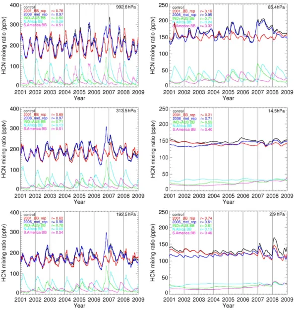
Fig. 7. GEOS-Chem HCN mixing ratios (pptv) averaged between 10◦S–10◦N during 2001–2008 in the troposphere (left panels) and the stratosphere (right panels): control experiment (black line); constant 2001 BB emissions experiment (red line); and constant 2006 meteorology experiment (dark blue line). Other colors denote HCN contributions from regional BB emissions: IND+AUS (green line), NAF (light blue line), and SA (purple line). The correlation coefficient r denotes the correlation between HCN mixing ratios and the total HCN mixing ratio of the control experiment; correlations >0.1 are statistically significant to the 99% confidence level.

budget in the lower and mid-troposphere than emissions from Africa (Fig. 7), resulting in anomalously large HCN concen-trations. The temporal overlapping of comparatively regular African BB emissions and emissions from other continents is key in establishing the apparent biennial cycle of HCN in the UTLS. This is consistent with Duncan et al. (2007) who showed that year-to-year of BB pollution in the UTLS are explained by year-to-year changes in BB from from In-donesia (here included in IND + AUS) and Central Amer-ica (here included in SA), particularly during El Ni˜no years when widespread fires occur over these regions.

Why is this transition between annual and biennial varia-tions not observed in other trace gases? This is probably due

to the atmospheric lifetime of the tracer being studied. For CO, with an atmospheric lifetime much less than HCN, es-pecially in the stratosphere, the signals due to surface emis-sions are too weak in the LS. For HCN, using the similar surface emission sources and ocean uptake sinks following Li et al. (2003), with the atmospheric sources of yields of CH3CN+OH (Kleinboehl et al., 2006) (see below) and

atmo-spheric sinks of chemical reactions with OH and O(1D), our model suggests a lifetime of 6.1 months. With this lifetime, the model reproduced the approximate 2-year cycle of HCN in the UTLS as observed by MLS and ACE-FTS, implying that our model source and sink estimates for HCN are appro-priate.

(11)

(a)

(b)

(c)

Fig. 8. Time series (solid line) of HCN biomass burning

emis-sion (Tg N/month) between 2001 and 2008 over (a) IND + AUS; (b) Africa (NAF + SAF); and (c) SA. Emissions above the 2001–2008 mean value are denoted by red triangles, and emissions 2.5 times above this mean value are denoted by blue squares. Emissions are based on GFEDv2 (van der Werf et al., 2006) and scaled using an observed HCN:CO emission ratio of 0.27% (Li et al., 2003). Verti-cal lines denote Verti-calendar years.

4.2 The HCN source from CH3CN+OH

As discussed above, our quantitative understanding of the HCN source from the oxidation of CH3CN by OH is

in-complete (Kleinboehl et al., 2006 and references therein). In our control simulation we used a 30% molar HCN yield that reconciled model calculations and balloon measurements at mid and high latitudes (Kleinboehl et al., 2006). This

atmo-spheric source of HCN is generally small in the troposphere (<1% of total HCN concentrations) but plays a larger role in the stratosphere (typically 5%), particularly at high latitudes (>7%). We find that including this HCN source does help to decrease (∼25%) the discrepancy between model and ACE-FTS observed HCN concentrations in the stratosphere (figure not shown) but does not improve further the model ability to capture observed HCN variations.

5 Concluding remarks

We have interpreted observed variations of HCN in the tropo-sphere and lower stratotropo-sphere using the GEOS-Chem global 3-D model of atmospheric chemistry and transport. We found that the observed annual and semi-annual variations in column HCN at three ground-based stations at low and mid-latitudes are described by the model with a positive bias of 5%. Using GEOS-Chem, we find that these variations are largely determined by biomass burning, with a number of su-perimposed regional burning signals in tropical latitudes. Us-ing HCN measurements from ACE-FTS and MLS, we found that in the UTLS the dominant period of variability is close to 24 months. We find this is true for the 36-month record from ACE-FTS and for the 52-month record from MLS which overlap our GEOS-Chem simulation. Using GEOS-Chem, we were able to reproduce only the broad observed distri-bution of HCN concentration typically with a negative bias of 20%, and the observed distribution of standard deviations of HCN concentrations with a similar value of ∼10 pptv in tropical UTLS, and the observed tropical variability typically with a negative bias of 7%, compared with the satellite ob-servations over the 52 months. Putting that observation pe-riod into a longer temporal perspective, by inspecting model variability from the previous four years, we observe a strong variability on a timescale of 24 months in the lower strato-sphere.

We find that tropical biomass burning is the largest sin-gle source of HCN and represents most of variability in the UTLS over the tropics, with the remainder of the variability due to atmospheric transport processes. Linking the quasi-biennial oscillation (QBO) and the UTLS HCN distribution is outside the scope of this study. We find that the extent of temporal overlap between African BB emissions and those from other continents, particular Indonesia, Australia and South America, is key in establishing the apparent biennial cycle in the UTLS. Transition from the annual and semi-annual variations of trace gases in the upper troposphere to the 2-year variation in the lower stratosphere has not been observed previously, perhaps due to the shorter lifetime of the other trace gases studied.

The main objective of this paper was to develop HCN as a reliable tracer for biomass burning, which we could then use to quantify BB emissions thereby helping to con-strain other sources. Without first reconciling the apparent

(12)

discrepancy between available observations it would be dif-ficult to achieve that objective. Using a global 3-D chemistry transport model was key in achieving this reconciliation. The model was able to reproduce the magnitude and variability of observed column concentrations over a limited number of available ground stations. GEOS-Chem was only able to re-produce the broad scale features of the HCN distributions ob-served by ACE-FTS and MLS but it successfully reproduced the timing and magnitude of observed fluctuations of HCN in the upper troposphere and lower stratosphere, reflecting the model ability to simulate atmospheric transport. Reducing the discrepancy between model and observed HCN concen-trations will require better constraints on the surface emis-sions and also on the atmospheric chemistry. We acknowl-edge that using upper tropospheric measurements of HCN to infer other sources will be difficult without better constraints on the rest of the troposphere. However, these observa-tions provide information about mechanisms of stratosphere-troposphere exchange (STE) of air and its origin, particularly if they are used in conjunction with concurrent measurements of CO and O3which we will explore in future work.

Acknowledgements. This work is funded by the UK Natural

Environmental Research Council (NERC) under NE/E003990/1. The ground-based FTIR data of HCN from Kitt Peak and Mauna Loa stations were provided by the NDACC network (http://www.ndacc.org). The ACE mission is primarily funded by the Canadian Space Agency. The ground-based FTIR data of HCN from Jungfraujoch station were provided by University of Li`ege. Primarily supported by the Belgian Federal Science Policy Office (PRODEX and SSD programs), Brussels. We acknowledge the International Foundation High Altitude Research Stations Jungfraujoch and Gornergrat (HFSJG, Bern, Switzerland) for allowing us to conduct our experiments at the High Altitude Re-search Station at Jungfraujoch. We also thank our colleagues from Harvard University who developed the GEOS-Chem capability of using GEOS-5 meteorology.

Edited by: B. N. Duncan

References

Baldwin, M. P., Gray, L. J., and Dunkerton, T. J.: The quasi-biennial oscillation, Rev. Geophys., 39, 179–229, 2001.

Bange, H. W. and Williams, J.: Acetonitrile in atmospheric and biogeochemical cycles, Atmos. Environ., 34, 4959–4990, 2000. Bernath, P. F., McElroy, C. T., Abrams, M. C., et al.: Atmospheric

Chemistry Experiment (ACE): Mission overview, Geophys. Res. Lett., 32, L15S01, doi:10.1029/2005GL022386, 2005.

Bertschi, I., Yokelson, R. J., Ward, D. E., Babbitt, R. E., Su-sott, R. A., Goode, J. G., and Hao, W. M.: Trace gas and particle emissions from fires in large diameter and be-lowground biomass fuels, J. Geophys. Res., 108(D13), 8472, doi:10.1029/2002JD002100, 2003.

Bey, I., Jacob, D. J., Yantosca, R. M., Logan, J. A., Field, B. D., Fiore, A. M., Li, Q., Liu, H. Y., Mickley, L. J., and Schultz, M. G.: Global modeling of tropospheric chemistry with

assim-ilated meteorology: Model description and evaluation, J. Geo-phys. Res., 106(D19), 23073–23095, 2001.

Boone, C. D., Nassar, R., Walker, K. A., Rochon, Y., McLeod, S. D., Rinsland, C. P., and Bernath, P. F.: Retrievals for the atmospheric chemistry experiment Fourier-transform spectrometer, Appl. Op-tics, 44, 7218–7231, 2005.

Brasseur, G., Zellner, De Rudder, R. A., and Arjis, E.: Is hydrogen cyanide a progenitor of acetonitrile in the atmosphere?, Geophys. Res. Lett., 12, 117–120, 1985.

Cicerone, R. J. and Zellner, R.: The Atmospheric Chemistry of Hydrogen Cyanide (HCN), J. Geophys. Res., 88(C15), 10689– 10696, 1983.

Duncan, B. N., Strahan, S. E., Yoshida, Y., Steenrod, S. D., and Livesey, N.: Model study of the cross-tropopause transport of biomass burning pollution, Atmos. Chem. Phys., 7, 3713–3736, 2007,

http://www.atmos-chem-phys.net/7/3713/2007/.

Fiore, A., Jacob, D. J., Liu, H., Yantosca, R. M., Fairlie, T. D., and Li, Q. B.: Variability in surface ozone background over the United States: Implications for air quality policy, J. Geophys. Res., 108(4787), doi:10.1029/2003JD003855, 2003.

Holton, J. R., Haynes, P. H., McIntyre, M. E., Douglass, A. R., Rood, R. B., and Pfister, L.: Stratosphere-Troposphere Ex-change, Rev. Geophys., 33(4), 403–439, 1995.

Holzinger, R., Warneke, C., Hansel, A., Jordan, A., and Lindinger, W.: Biomass burning as a source of formaldehyde, acetaldehyde, methanol, acetone, acetonitrile, and hydrogen cyanide, Geophys. Res. Lett., 26(8), 1161–1164, 1999.

Holzinger, R., Jordan, A., Hansel, A., and Lindinger, W.: Automo-bile emissions of acetonitrile: Assessments of its contribution to the global sources, Atmos. Environ., 38, 187–193, 2001. Jacob, D. J., Crawford, J., Kleb, M. M., Connors, V. S., Bendura,

R. J., Raper, J. L., Sachse, G. W., Gille, J., Emmons, L., and Heald, J. C.: Transport and Chemical Evolution over the Pacific (TRACE-P) mission: Design, execution, and first results, J. Geo-phys., Res., 108(D20), 9000, doi:10.1029/2002JD003276, 2003. Kleinboehl, A., Toon, G. C., Sen, B., et al.: On the stratospheric chemistry of hydrogen cyanide, Geophys. Res. Lett., 33, L11806, doi:10.1029/2006GL026015, 2006.

Li, Q., Jacob, D. J., Bey, I., Yantosca, R. M., Zhao, Y., Kondo, Y., and Notholt, J.: Atmospheric hydrogen cyanide (HCN): Biomass burning source, ocean sink?, Geophys. Res. Lett., 27(3), 357– 360, 2000.

Li, Q., Jacob, D. J., Yantosca, R. M., Heald. C. L., Singh, H. B., Koike, M., Zhao, Y., Sachse, G. W., and Streets, D. G.: A global three-dimensional model analysis of the atmo-spheric budgets of HCN and CH3CN: Constraints from aircraft

and ground measurements, J. Geophys. Res., 108(D21), 8827, doi:10.1029/2002JD003975, 2003.

Liu, C. and Zipser, E. J.: Global distribution of convection pene-trating the tropical tropopause, J. Geophys. Res., 110, D23104, doi:10.1029/2005JD006063, 2005.

Lobert, J. M., Scharffe, D. H., Hao, W. M., and Crutzen, P. J.: Importance of biomass burning in the atmospheric budgets of nitrogen-containing gases, Nature, 346, 552–554, 1990. Logan, J. A., Jones, D. B. A., Megretskaia, I. A., et al.:

Quasibiennial oscillation in tropical ozone as revealed by ozonesonde and satellite data, J. Geophy. Res., 108(D8), 4244, doi:1029/2002JD002170, 2003.

(13)

Lupu, A., Kaminski, J. W., Neary, L., McConnell, J. C., Toyota, K., Rinsland, C. P., Bernath, P. F., Walker, K. A., Boone, C. D., Nagahama, Y., and Suzuki, K.: Hydrogen cyanide in the upper troposphere: GEM-AQ simulation and comparison with ACE-FTS observations, Atmos. Chem. Phys., 9, 4301–4313, 2009, http://www.atmos-chem-phys.net/9/4301/2009/.

Mahieu, E., Rinsland, C. P., Zander, R., Demoulin, P., Delbouille, L., and Roland, G.: Vertical Column Abundances of HCN De-duced from Ground-Based Infrared Solar Spectra: Long-Term Trend and Variability, J. Atmos. Chem., 20, 299–310, 1995. Mahieu, E., Zander, R., Delbouille, L., Demoulin, P., Roland, G.,

and Servais, C.: Observed trends in total vertical column abun-dances of atmospheric gases from IR solar spectra recorded at the Jungfraujoch, J. Atmos. Chem., 28, 227–243, 1997. Martin, R. V., Jacob, D. J., Logan, J. A., et al.: Interpretation of

TOMS observations of tropical tropospheric ozone with a global model and in situ observations, J. Geosphys. Res., 107(D18), 4351, doi:10.1029/2001JD001480, 2002.

Mote, P. W., Rosenlof, K. H., McIntyre, M. E., et al.: An atmo-spheric tape recorder: The imprint of tropical tropopause temper-atures on stratospheric water vapor, J. Geophys. Res, 101(D2), 3989–4006, 1996.

Park, R. J., Jacob, D. J., Field, B. D., Yantosca, R. M., and Chin, M.: Natural and transboundary pollution influ-ences on sulface-nitrate-ammonium aerosols in the United States: Implications for policy, J. Geophys. Res., 109, D15204, doi:10.1029/2003JD004473, 2005.

Pickett, H. M., Read, W. G., Lee, K. K., and Yung, Y. L.: Obser-vation of night OH in the mesosphere, Geophys. Res. Lett., 33, L19808, doi:10.1029/2006GL026910, 2006.

Pickett, H. M., Drouin, B. J., Canty, T., et al.: Validation of Aura Microwave Limb Sounder OH and HO2measurements, J.

Geo-phys. Res., 113, D16S30, doi:10.1029/2007JD008775, 2008. Plumb, R. A. and Bell, R. C.: A model of the quasi-biennial

oscilla-tion on an equatorial beta-plane, Q. J. Roy. Meteorol. Soc., 108, 335–352, 1982.

Pumphrey, H. C., Jimenez, C. J., and Waters, J. W.: Measurement of HCN in the middle atmosphere by EOS MLS, Geophys. Res. Lett., 33(8), L08804, doi:10.1029/2005GL025656, 2006. Pumphrey, H. C., Boone, C., Walker, K. A., Bernath, P., and

Liv-ersey, N. J.: Tropical tape recorder observed in HCN, Geophys. Res. Lett., 35, L05801, doi:10.1029/2007/GL032137, 2008. Randel, W. and Wu, F.: Isolation of the ozone QBO in SAGE II data

by singular-value decomposition, J. Atmos. Sci., 53, 2546–2559, 1996.

Randel, W. J., Wu, F., Russell III, J. M., Roche, A., and Waters, J. W.: Seasonal Cycle and QBO Variations in Stratospheric CH4

and H2O Observed in UARS HALOE Data, J. Atmos. Sci., 55,

163–185, 1998.

Randel, W. J. and Wu, F.: A stratospheric ozone profile data set for 1979–2005: Variability, trends, and comparison with column ozone data, J. Geosphy. Res., 112, D06313, doi:10.1029/2006JD007339, 2007.

Rinsland, C. P., Goldman, A., Murcray, F. J., et al.: Infrared so-lar spectroscopic measurements of free tropospheric CO, C2H6,

and HCN above Mauna Loa, Hawaii: Seasonal variations and evidence for enhanced emissions from the Southeast Asian trop-ical fires 1997–1998, J. Geophys. Res., 104(D15), 18667–18680, 1999.

Rinsland, C. P., Mahieu, E., Zander, R., Demoulin, P., Forrer, J., and Buchmann, B.: Free tropospheric CO, C2H6, and HCN above

central Europe: Recent measurements from the Jungfraujoch sta-tion including the detecsta-tion of elevated columns during 1998, J. Geophys. Res., 105(D19), 24235–24249, 2000.

Rinsland, C. R., Goldman, A., Zander, R., and Mahieu, E.: En-hanced tropospheric HCN columns above Kitt Peak during the 1982–1983 and 1997–1998 El Nino warm phases, J. Quant. Spectrosc. Ra., 69, 3–8, 2001.

Rinsland, C. P., Goldman, A., Hannigan, J. W., Wood, S. W., Chiou, L. S., and Mahieu, E.: Long-term trends of tropospheric carbon monoxide and hydrogen cyanide from analysis of high resolu-tion infrared solar spectra, J. Quant. Spectrosc. Ra., 104, 40–51, 2007.

Schneider, J., Burger, V., and Arnold, F.: Methyl cyanide and hy-drogen cyanide measurements in the lower stratosphere: Impli-cations for methyl cyanide sources and sinks, J. Geophys. Res., 102(D21), 25501–25506, 1997.

Schoeberl, M. R., Roche, A. E., Russell III, J. M., Ortland, D., Hays, P. B., and Waters, J. W.: An estimation of the dynamical isolation of the tropical lower stratosphere using trace gas observations of the quasi-biennial oscillation, Geophys. Res. Lett., 24, 53–56, 1997.

Schoeberl, M. R., Duncan, B. N., Douglass, A. R., Waters, J., Liversey, N., Read, W., and Filipiak, M.: The carbon monoxide tape recorder, Geophys. Res. Lett., 33, L12811, doi:10.1029/2006GL026178, 2006.

Schoeberl, M. R., Douglass, A. R., Newman, P. A., et al.: QBO and annual cycle variations in tropical lower stratosphere trace gases from HALOE and Aura MLS observations, J. Geophys. Res., 113, D05301, doi:10.1029/2007JD008678, 2008.

Singh, H. B., Salas, L., Herlth, D., et al.: In situ mea-surements of HCN and CH3CN over the Pacific Ocean:

Sources, sinks and budgets, J. Geophys. Res., 108, 8795, doi:10.1029/2002JD003006, 2003.

Streets, D. G., Bond, T. C., Carmichael, G. R., et al.: An inventory of gaseous and primary aerosol emissions in Asia in the year 2000, J. Geophys. Res., 108(D21), 8809, doi:10.1029/2002JD003093, 2003.

van der Werf, G. R., Randerson, J. T., Giglio, L., Collatz, G. J., Kasibhatla, P. S., and Arellano Jr., A. F.: Interannual variability in global biomass burning emissions from 1997 to 2004, Atmos. Chem. Phys., 6, 3423–3441, 2006,

http://www.atmos-chem-phys.net/6/3423/2006/.

Wand, M. P. and Jones, M. C.: Kernel Smoothing, Chapman and Hall, London, UK, 1995.

Waters, J. W.: The Earth Observing System Microwave Limb Sounder (EOS MLS) on the Aura satellite, IEEE T. Geosci. Re-mote, 44(5), 1106–1121, 2006.

Zhao, Y., Kondo, Y., Murcray, F. J., et al.: Seasonal variations of HCN over northern Japan measured by ground-based infrared solar spectroscopy, J. Geophys. Res., 27, 2085–2088, 2000. Zhao, Y., Strong, K., Kondo, Y., et al.: Spectroscopic measurements

of tropospheric CO, C2H6, C2H2, and HCN in northern Japan,

J. Geophys. Res., 107(D8), 4343, doi:10.1029/2001JD000748, 2002.