An experiment on the parameter uncertainty of
hydrological models with different levels of complexity
in a climate change context.
Thèse
Slim Kouki
Doctorat en génie civil
Philosophiæ doctor (Ph.D.)
Québec, Canada
RÉSUMÉ
La possibilité d’estimer l’impact du changement climatique en cours sur le comportement hydrologique des hydro-systèmes est une nécessité pour anticiper les adaptations inévitables et nécessaires que doivent envisager nos sociétés. Dans ce contexte, ce projet doctoral présente une étude sur l'évaluation de la sensibilité des projections hydrologiques futures à :
(i) La non-robustesse de l’identification des paramètres des modèles hydrologiques, (ii) l’utilisation de plusieurs jeux de paramètres équifinaux et (iii) l’utilisation de différentes structures de modèles hydrologiques.
Pour quantifier l’impact de la première source d’incertitude sur les sorties des modèles, quatre sous-périodes climatiquement contrastées sont tout d’abord identifiées au sein des chroniques observées. Les modèles sont calés sur chacune de ces quatre périodes et les sorties engendrées sont analysées en calage et en validation en suivant les quatre configurations du Different
Split-sample Tests (Klemeš, 1986;Wilby, 2005; Seiller et al. (2012);Refsgaard et al.
(2014)). Afin d’étudier la seconde source d’incertitude liée à la structure du modèle, l’équifinalité des jeux de paramètres est ensuite prise en compte en considérant pour chaque type de calage les sorties associées à des jeux de paramètres équifinaux. Enfin, pour évaluer la troisième source d'incertitude, cinq modèles hydrologiques de différents niveaux de complexité sont appliqués (GR4J, MORDOR, HSAMI, SWAT et HYDROTEL) sur le bassin versant québécois de la rivière Au Saumon. Les trois sources d'incertitude sont évaluées à la fois dans conditions climatiques observées passées et dans les conditions climatiques futures.
Les résultats montrent que, en tenant compte de la méthode d'évaluation suivie dans ce doctorat, l'utilisation de différents niveaux de complexité des modèles hydrologiques est la principale source de variabilité dans les projections de débits dans des conditions climatiques futures. Ceci est suivi par le manque de robustesse de l'identification des paramètres. Les projections hydrologiques générées par un ensemble de jeux de paramètres équifinaux sont proches de celles associées au jeu de paramètres optimal. Par conséquent, plus d'efforts devraient être investis dans l'amélioration de la robustesse des modèles pour les études d'impact sur le changement climatique, notamment en développant les structures des modèles plus appropriés et en proposant des procédures de calage qui augmentent leur robustesse.
Ces travaux permettent d’apporter une réponse détaillée sur notre capacité à réaliser un diagnostic des impacts des changements climatiques sur les ressources hydriques du bassin Au Saumon et de proposer une démarche méthodologique originale d’analyse pouvant être directement appliquée ou adaptée à d’autres contextes hydro-climatiques.
ABSTRACT
The possibility to estimate the impact of climate change on the hydrological behavior of hydrosystems, the hydrological risks, and the associated resources is a necessity in order to anticipate the inevitable and necessary adaptations that must consider our societies.
In this context, the doctoral project presents a study on the evaluation of the uncertainty of hydrological projections for the future climate when considering: (i) The non-robustness of hydrological model parameter identification, (ii) the use of several ensembles of equifinal parameter sets over a given calibration period and (iii) the use of different model structures for the hydrological model.
To quantify the impact of the first source of uncertainty on the model outputs, four climatically contrasted sub-periods are first identified within the observed time series. The models are calibrated on each of these four periods, then generated outputs are analyzed on calibration and validation data. The calibration and validation tests were performed according to the configurations of four Different Split-sample Tests (Klemeš, 1986; Wilby, 2005; Seiller et al., 2012; Refsgaard et
al., 2014). In order to study the second source of uncertainty related to the model
structure, the equifinality of the parameter sets is taken into account by considering an ensemble of equifinal parameter sets for each sub-period calibration. Finally, to assess the third source of uncertainty, five hydrological models of different levels of complexity are applied (GR4J, MORDOR, HSAMI, SWAT, and HYDROTEL) on the watershed of the Au Saumon River (Québec, Canada).The three sources of uncertainty are assessed in the past observed period and in future climate conditions.
Results show that, given the evaluation approach followed in this Ph.D. research,
the use of different levels of complexity of hydrological models is the major source of variability in streamflow projections in future climate conditions for the five models tested. This is followed by the lack of robustness of parameter identification. The hydrological projections generated by an ensemble of equifinal parameter sets are close to those associated with the optimal set. Therefore, it seems that greater effort should be invested in improving the robustness of models for climate change impact studies, especially by developing more suitable model structures and proposing calibration procedures that increase their robustness. This work serves to provide a detailed response on our ability to make a diagnosis of the impacts of climate change on water resources of the Au Saumon watershed and proposes a novel methodological approach that can be directly applied or adapted to other hydro-climatic contexts.
TABLE OF CONTENTS
RÉSUMÉ ... iii ABSTRACT ... v TABLE OF CONTENTS ... vii LIST OF FIGURES ... xi LIST OF APPENDICES ... xv REMERCIEMENTS (ACKNOWLEDGEMENTS) ... xvii GENERAL INTRODUCTION ... 1 CONTEXT ... 3 PROBLEM STATEMENT ... 4ORGANIZATION OF THE THESIS ... 6
Chapter 1. Literature review and Objectives ... 8
1.1. ... Uncertainties related to the use of hydrological models in changing climate ... 8
1.1.1. Climatic uncertainties ...10
1.1.2. Hydrological uncertainties ...17
1.1.3. Quantification of these two sources of uncertainties ...19
1.2. ... Uncertainties related to the parameters of the hydrological models ... 20
1.2.1. Robustness of the parameter identification ...21
1.2.2. The concept of equifinality and the Generalized Likelihood Uncertainty Estimate (GLUE) method ...25
1.3. ... Research objectives ... 26
1.3.1. Objective 1: Evaluation of the temporal transposability of five different hydrological models under contrasted climates and evaluation of the extent of the equifinality of their parameter sets. ...27
1.3.2. Objective 2: To what extent does the selection of a parameter set for a hydrological model influence its hydrological projections? ...28
1.3.3. Objective 3: Does higher complexity in hydrological modelling infer less uncertain hydrological projections? ...29
Chapter 2. General methodology ... 33
2.1. Preliminary remarks and definitions ... 33
2.2 Data and models ... 34
2.2.1 Catchment ...35
2.2.2. Hydro-meteorological data ...38
2.2.3. Hydrological models ...40
2.5. General methodology for investigating parameter uncertainty in a changing
climate ... 49
2.5.1 Step 1: Identification of climatically contrasted sub-periods ...50
2.5.2 Step 2: Implementation of sub-period calibration/validation and identification of equifinal parameter sets ...53
2.5.3 Step 3: Simulation, projection, and parametric identification uncertainties quantification ...60
Chapter 3. Evaluation of the temporal transposability of five hydrological models under contrasted climates and of the extent of the equifinality of their parameters sets ... 68
3.1. Challenges and Objectives ... 68
3.2. Evaluation of temporal transposability of the selected hydrological models ... 69
3.2.1. Analysis on calibration and validation performance of four DSSTs ...70
3.3. Associated parametric uncertainty related to equifinality of parameters ... 75
3.3.1. Impact of climate specificity of calibration period on the identified equifinal parameter values ...76
3.3.2. Analysis on the performance of equifinal parameter sets on DSST’s sub-periods ...79
3.3.3 Impact of equifinality on the outputs of hydrological models ...81
3.4. Synthesis and discussion ... 89
Chapter 4. To what extent does the selection of a parameter set for a hydrological model influence hydrological projections? ... 92
4.1. Sensitivity to the climate characteristics of the calibration period ... 92
4.1.1. Assessment on the representation of the current climate ...93
4.1.2. Impacts on simulated flow evolutions ...100
4.2. Sensitivity to the use of an equifinal ensemble of parameter sets ... 105
4.2.1. Sensitivity on current climate ...105
4.2.2. Impacts on simulated flows ...111
4.3. Synthesis and Discussion ... 114
Chapter 5: Does higher complexity in hydrological modelling infer less uncertain hydrological projections? ... 117
5.1. Challenges and Objectives ... 117
5.2. Sensitivity to the choice of the hydrological model ... 118
5.2.1. Impact on the modelling performance ...118
5.2.2. Impact on simulated and projected discharges ...122
5.2.3. Impact on hydrological indicators ...128
5.3. Synthesis and Discussion ... 136
GENERAL CONCLUSION ... 139
BIBLIOGRAPHY ... 145
LIST OF TABLES
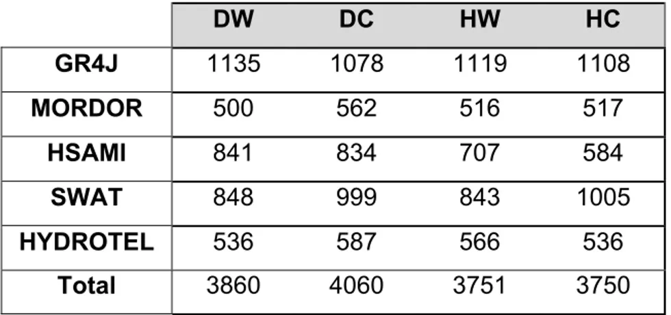
Table 1 - Main characteristics of the five selected models. ... 40 Table 2 - Characteristics of the DSST periods (DW: dry/warm; DC: dry/cold; HW:
humid/warm; HC: humid/cold) ... 53 Table 3 - Number of identified equifinal parameter sets for each hydrological model. ... 76 Table 4 – SPREAD RMSE Ratio (SRR) in calibration and in validation. ... 89 Table 5 - Changes of hydrological indicators from reference to future period. ... 136
LIST OF FIGURES
Figure 1 - Schematic view of the cascading uncertainties that are subject to the hydrological projections in the context of climate change. ... 10 Figure 2 - Schematic representation of the four main families of SRES scenarios
(Source: IPCC: (Nakićenović et al., 2000)). ... 11 Figure 3 – General description of the methods applied in the Ph.D. research. The details of the methodology are explained in Chapter 2. ... 32 Figure 4 - Location and characteristics of the Au Saumon catchment (738 km2). ... 36
Figure 5 – Observed meteorological and hydrometric interannual data (1975-2003). .... 37 Figure 6 - CRCM domain for the studied watershed, in yellow (Haut-Saint-François
Basin). (Source: Project of QBIC3) ... 39
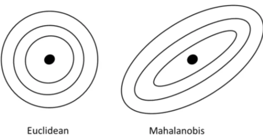
Figure 7 - Identification of DSST years. ... 51 Figure 8 - The different contours for constant Euclidean and Mahalanobis metrics in 2D
space (Lenoir and Beaugrand, 2008). ... 57 Figure 9 - Analysis of sensitivity of hydrological projections to the parameter sets
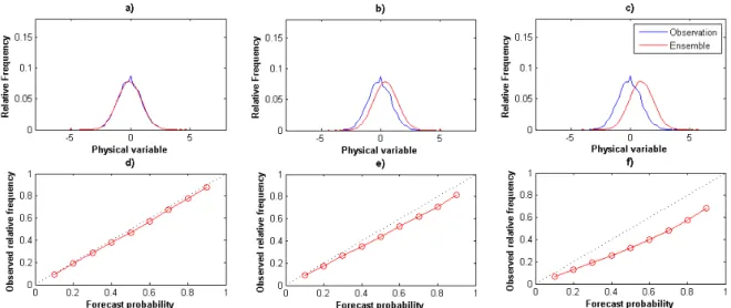
identification and equifinality. ... 62 Figure 10 - Hypothetical probability density functions for a given observed variable and
its ensemble prediction along with their associated reliability diagrams for: (a) Underdispersed PDF, (b) Well-calibrated PDF, (c) Overdispersed PDF, (d) Reliability diagram corresponding to (a), (e) Reliability diagram corresponding to (b) and (f) Reliability diagram corresponding to (c). ... 65 Figure 11 - Hypothetical probability density functions for a given observed variable and
its ensemble prediction, with different mean values, along with their associated reliability diagrams for: (a) Well-calibrated PDF with same mean, (b) Biased PDF, (c) Very biased PDF, (d) Reliability diagram corresponding to (a), (e) Reliability diagram corresponding to (b) and (e) Reliability diagram corresponding to (c). ... 65 Figure 12 - Performances and rank in calibration and validation of the five hydrological
models for the four DSST (full circle for calibration and full square for validation). . 72 Figure 13 - Cumulative error between observed and simulated discharges for all the DSS tests in validation. ... 74 Figure 14 - Comparison between mean daily interannual discharges for four DSSTs in
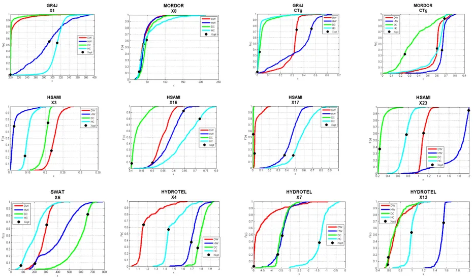
Figure 15 - Distributions of selected parameter values obtained according to the calibration conditions for the five models. ... 78 Figure 16 - Distributions of absPVE (%), NSE, NSEsqrt and NSElog, values obtained for the
five hydrological models illustrating their validation performance over the DSSTs. The black asterisks on the boxplots show the performance of the optimal parameter set obtained in validation. ... 80 Figure 17 - Mean daily interannual discharges for DWHC’s DSST validation of
equifinal parameter sets of the HYDROTEL model. ... 82 Figure 18 - Reliability diagrams of the 4 ensembles of discharges using 4 ensembles of
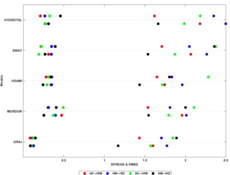
equifinal parameter sets on opposite validation periods. ... 86 Figure 19 - RMSE (square) vs Spread (circle) of equifinal ensembles in calibration and in validation. ... 88 Figure 20 - Calibration and validation performance values of the five models obtained
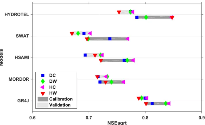
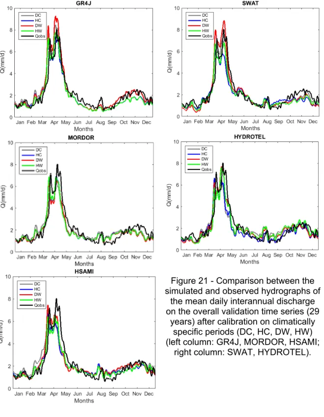
over the entire observed period for the 4 different calibrations. ... 94 Figure 21 - Comparison between the simulated and observed hydrographs of the mean
daily interannual discharge on the overall validation time series (29 years) after calibration on climatically specific periods (DC, HC, DW, HW) (left column: GR4J, MORDOR, HSAMI; right column: SWAT, HYDROTEL). ... 96 Figure 22 - Sensitivity of the simulated hydrographs of the mean daily interannual
discharge on the overall validation time series (29 years) after calibration on climatically specific periods (DC, HC, DW, HW) (left column: GR4J, MORDOR, HSAMI; right column: SWAT , HYDROTEL). The Q-Q plots show the observed versus simulated values, each dot representing the mean of values simulated with the four optimal parameter sets and each bar representing the range of simulated values when using the four optimal parameter sets. The boxplots on the right represent the distributions of the relative errors on the flow characteristics on the overall record validation. ... 99 Figure 23 - Comparison between simulated and observed hydrographs of the mean daily interannual discharge on the climatic data (REF: solid line, FUT: dashed line) after calibration on climatically specific periods (DC, HC, DW, HW) (left column: GR4J, MORDOR, HSA MI; right column: SWAT, HYDROTEL). ... 101 Figure 24 - Comparison of the simulations of the mean daily interannual discharge
obtained on the reference period (REF) and future period (FUT) under projected climate conditions with the five hydrological models (left: GR4J, MORDOR, HSAMI;
right: SWAT, HYDROTEL). Horizontal bars represent the variation (min-max) of interannual mean daily discharges simulated over REF, while the vertical bars represent its variation on FUT. The intersection between the two bars represents the
average of the four simulated flows over REF and FUT (4 x Xopt). Beside each
intersection it is mentioned the number of day, from 1 to 365 days. ... 104 Figure 25 - Lissajous-Bowditch curves showing the interannual mean hydrographs
simulated on REF and FUT with the five hydrological models. ... 105 Figure 26 - Distribution of NSEsqrt values obtained with the five models illustrating
validation performance over all data (29 years) and equifinal parameters sets identified on four different climatic conditions in calibration. ... 107 Figure 27 - Mean daily interannual flows simulated with 4 ensembles of equifinal
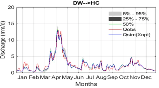
parameter sets (four period calibrations: DW, HC, DC and HW) on all observed time series. For each ensemble of equifinal parameter sets, the grayscale zone represent the extent of the equifinality uncertainty (5%-95%, 25% to 75%), the median is given in green, the observations in red and the "optimal" simulation in blue (outcome of an optimal set of parameters calibrated in the same sub-period). ... 110 Figure 28 - Mean daily interannual discharges simulated with 4 ensembles of equifinal
parameter sets (four sub-period calibrations: DW, HC, DC and HW) on reference (REF) and future (FUT) periods (for the five models). ... 113 Figure 29 - Classification of the complexity of hydrological models and their associated
performances with NSEsqrt for CAL and the four DSST. ... 120
Figure 30 - Classification of the complexity of hydrological models and their associated performances with absPVE for CAL and the four DSST. ... 122 Figure 31 – Comparison between the envelopes of the mean daily interannual
discharges simulated by lumped models (GR4J, MORDOR and HSAMI) in dark blue and process-based semi-distributed models (SWAT and HYDROTEL) in light blue. ... 124 Figure 32 - Envelopes of mean daily interannual discharges on periods REF (top) and
FUT (bottom), for the 5 available member climates combined (MC). The blue envelope represents the sensitivity of the 3 conceptual models (GR4J, MORDOR and HSAMI), the green envelope represents the process-based, semi-distributed models (SWAT AND HYDROTEL). ... 126 Figure 33 - Quantile-Quantile plots of simulated discharges series (Quantiles values in
models. The gray lines identify the 50% quantile. The blue lines represent the regression lines. The extent of each graph corresponds to the 90% quantile. ... 127 Figure 34 – The Overall Mean Flow (OMF) calculated for the available observed time
series and the four DSST in validation. ... 130 Figure 35 - The 2-yr return period 7-day low flow (Q2,7) calculated on a) Winter and on b)
Summer for the available observed time series and the four DSST in validation. . 131 Figure 36 - The 2-yr return period high flow (Q2) calculated on a) Spring and b) Fall for
the available observed time series and the four DSST in validation. ... 133 Figure 37 - Values of hydrological indicators (mm/d) in reference [5 x (1971-2000)] and
future [5x(2041-2070)] period of overall mean flow (OMF), the 2-yr return period 7-day low flow (Q2,7) in summer and winter, and the 2-yr return period high flow (Q2) in
Spring and Fall. ... 136
LIST OF APPENDICES
APPENDIX A - Characteristics of conceptual Hydrological Models used in the project. ... 172 APPENDIX B - Impact of climate specificity of the calibration condition on the value of
the parameters. ... 177 APPENDIX C - Impact of the equifinality of parameter sets on the outputs of hydrological models in validation ... 193
REMERCIEMENTS (ACKNOWLEDGEMENTS)
Le Doctorat est l’achèvement d’une réflexion originale et de longue haleine, je tiens donc dans ces quelques lignes à remercier les gens qui ont compté pour moi durant ces 5 années de travail.
Je tiens à remercier chaleureusement mon directeur de thèse, M. François Anctil, directeur de l’institut EDS et professeur titulaire du Département de génie civil et de génie des eaux de l’Université Laval, pour sa disponibilité, son efficacité, et pour la confiance qu'il m'a accordé. Tout au long de mon périple de doctorat, tu as été présent pour répondre à mes interrogations et inquiétudes. Tu as su me prodiguer des conseils constructifs durant mes quatre années de Doctorat.
J’adresse ma gratitude aux membres du jury qui ont accepté de commenter et critiquer ce travail de doctorat, à savoir : M. Richard Turcotte, chef de la division de l’hydrologie et de l’hydraulique, adjoint à la Direction de l’expertise hydrique « volet scientifique » au Centre d’expertise hydrique du Québec (CEHQ) et coordonnateur des activités du programme « Ressources hydriques » du Consortium Ouranos (Canada); Mme. Geneviève Pelletier et M. Peter Vanrolleghem, professeurs du Département de génie civil et de génie des eaux de l’Université Laval.
Je remercie également les différents professeurs du Département de génie civil et de génie des eaux de l'Université Laval qui ont suivi et validé les étapes d'avancement de mon doctorat : M. Paul Lessard et M. Amaury Tilmant.
Je tiens aussi à mettre en évidence que ces travaux n'auraient pas été réalisables sans la collaboration des personnes qui ont permis de faire avancer ce travail dans d'excellentes conditions au niveau technique et scientifique, pour leur partage de données, d'outils ou de connaissances, à savoir : Simon Lachance-Cloutier, Simon Ricard et Thomas-Charles Fortier-Filion du CEHQ; Daniel Caya, Diane Chaumont, David Huard, Blaise Gauvin-St Denis et Juan-Alberto Velázquez Zapata d'Ouranos; Catherine Guay et Marie Minville de l'Institut de Recherche Hydro-Québec; Ralf Ludwig, Markus Muerth, Seppo Schmid et Sasha Berger de l'Université Ludwig-Maximilians de Munich.
Je remercie également chaleureusement Alain Royer de l’INRS, pour son partage d'outils de modélisation (HYDROTEL) et conseils associés.
Mes sincères remerciements à toutes les personnes rencontrées lors des colloques et conférences auxquels j'ai eu le plaisir d'assister et qui ont su valoriser et donner un sens au travail réalisé par leurs commentaires constructifs et leurs idées.
Un grand merci aux collègues de l'Université Laval qui ont fait de ces cinq ans de doctorat une expérience trop courte, je pense notamment à: Greg, Darwin,
Annie-Claude, Flora, Anne, Antoine, Benoît, Jérôme, Étienne, Sovanna, Marinella, Marie-Amélie, Lucas, Cyril, Renaud, Philipp, Arinala, Youen,... Merci bien sûr à tous ceux et celles que j'ai oublié de nommer.
Sur une note plus personnelle, j'aimerais remercier du fond du cœur ma famille : mes parents, Salha & Hédi, mon grand frère Walid, mes petites sœurs Ichraf & Amira, pour leur soutien, distant mais réel, tout au long de mon périple académique depuis ma douce Tunisie, en passant par Paris pour compléter ma maîtrise et finalement à la ville de Québec pour réaliser mon Doctorat. Sans vous, je ne serais probablement pas parvenue à achever la boucle et je vous en suis très reconnaissant. Une spéciale dédicace à mes anges: mon neveu Mohamed Aziz et ma nièce Mayssem. Un grand merci aussi à toute ma grande famille (les familles Kouki et Belkhir), évidemment. Pas besoin de vous énumérer, vous savez que je vous porte tous en moi quelque part.
Dans le même ordre d'idées, je tiens à remercier haut et fort ma femme Soaad, qui, surtout durant les dernières années, a dû mettre les bouchées doubles au travail pour me permettre d'être sur les bancs de l’université. Merci de prendre soin de moi, merci d'être là dans les moments difficiles et de me comprendre dans les périodes plus stressantes. De tout cela et de bien d'autres choses encore, je te suis très reconnaissant. Toi et mon fils que j’attends avec impatience, vous mettez du soleil dans ma vie et je vous aime très fort. Évidemment un merci particulier à ma belle-famille.
À tous, MERCI ! et pour ceux qui ont le courage d'aller plus loin et ne pas seulement s'arrêter aux remerciements pour voir si leur nom apparaît : BONNE LECTURE !
﴿ ْأَﺮْـﻗا ﻖَﻠَﺧ يِﺬﱠﻟا َﻚﱢﺑَر ِﻢْﺳﺎِﺑ ) 1 ( ٍﻖَﻠَﻋ ْﻦِﻣ َنﺎَﺴﻧِﻹا َﻖَﻠَﺧ ) 2 ( ُمَﺮْﻛَﻷا َﻚﱡﺑَرَو ْأَﺮْـﻗا ) 3 ( يِﺬﱠﻟا ِﻢَﻠَﻘْﻟﺎِﺑ َﻢﱠﻠَﻋ ) 4 ( ْﻢَﻠْﻌَـﻳ َْﱂ ﺎَﻣ َنﺎَﺴﻧِﻹا َﻢﱠﻠَﻋ ) 5 ( ﴾ نآرقلا ميركلا ] ةروس قلعلا [5-1:
Au nom d'Allah, le Tout Miséricordieux, le Très Miséricordieux. (1) Lis, au nom de ton Seigneur qui a créé, (2) qui a créé l'homme d'une adhérence. (3) Lis! Ton Seigneur est le Très Noble, (4) qui a enseigné par la plume [le calame], (5) a enseigné à l'homme ce qu'il ne savait pas. [Le Coran, Al‐Alaq: 1‐5]
In the name of Allah, the Entirely Merciful, the Especially Merciful. (1) Recite in the name of your Lord who created (2) Created man from a clinging substance. (3) Recite, and your Lord is the most Generous (4) Who taught by the pen (5) Taught man that which he knew not [The Quran, Al‐Alaq: 1‐5] يدھأ هذھ هاروتكدلا ىلإ ىلغأ يش ء يف يتايح يّمأ ةحيلص يبأو يداھلا ناذّللا ينامھلأ ةرباثملا يف سارّدلا ة ذنم رغّصلا ملو لاخبي ّيلع ًاموي ءيشب . لوقأ امھل : متنأ ينومتبھو ةايحلا لملأاو ةأشنلاو ىلع فغش ملعلا او ةفرعمل يتوخإ ىلإ و ةّرق ينيع : ،ديلو فارشإ و ةريمأ ىلإ يتجوز نوصملا داعس يلفطو يذلا ،يتأيس لوقأ امھل يتايح نل نوكت لمجأ امكنودب ىلإ لك نم ينملع ًافرح حبصأ انس هقرب ءيضي قيرطلا يمامأ
GENERAL INTRODUCTION
“The future depends on what you do today.” ― Mahatma Gandhi
CONTEXT
The Fifth Assessment Report (AR5) of the Intergovernmental Panel on Climate Change (IPCC, 2014) confirms that climate change will exacerbate the pressure on water resources. Different uses of the resource such as power generation and drinking water are particularly likely to be affected; trends in hydrometeorological variables have already been observed and further changes are projected.
In hydrology, the assessment of the impacts of changing climate demands the combined usage of 1) a global circulation model (GCM), of 2) downscaling techniques to reconcile the scale mismatch between the GCMs and the catchment scale, and of 3) a hydrological model. If lots of efforts have already targeted reducing the uncertainty of the first two components of such system, little quantitative knowledge is as yet available about the role of the hydrologic model structure and its parameter estimates.
In Canada, and more specifically in the province of Québec, significant trends in meteorological variables have been observed in the recent past (Yagouti et al., 2008; DesJarlais and Blondlot, 2010). Anticipated impacts of climate change on streamflows in Québec are periodically evaluated by two partners of this thesis: Hydro-Québec (HQ) throughout the province as well as by the Centre d’expertise
hydrique du Québec (CEHQ, Ministry of Sustainable Development, Environment
and the Fight against Climate Change) for the southern part of Québec.
In March 2013, the CEHQ has published the first edition of the Hydroclimatic
atlas (CEHQ, 2013) depicting the projected changes in high and low flows for the
2050 horizon. The data used in the assessment comprise a total of 89 climate projections (direct outputs or post-processed) and the modelling domain consisted of a region called meridional Québec which includes the Au Saumon watershed, the case study of this thesis. The 2015 edition of the Atlas (CEHQ, 2015) is the first in a series of updates that incorporate the most recent advances of research into hydroclimatic modelling.
The Hydroclimatic atlas (CEHQ, 2013, 2015) presents a synthesis of the state of knowledge describing the expected impact of climate change on the southern Québec water regime. The information presented in the atlas is based on the analysis of a change signal in the hydrological projections. This analysis is accompanied by a systematic assessment of associated uncertainties due to the use of GCMs, different techniques of downscaling, and global calibration. However, the analysis and the assessment of the uncertainties surrounding the hydrological model parameters and the choice of hydrological model structure is much more needed to more effectively support planning and implementing adaptation to climate change in Québec.
PROBLEM STATEMENT
This research project fits in the context previously exposed and aims to fill in the knowledge of uncertainties related to the use of projection tools. More generally, the posed problem is to explore:
What is our ability to produce a diagnosis of the impact of climate change on the water balance of a watershed of interest?
A hydrological model simulates future watershed outflows under downscaled actual and future climate projections. There is a huge array of hydrological models available (e.g. semi-distributed model and lumped model) that could accomplish this task. Many such models resort to conceptual descriptions of the hydrological processes that simplify their implementation but ask for the calibration of a number of internal unknown parameters.
Values of the parameters depend on objective function(s) and optimisation method used in the calibration, data errors (measurement errors and inadequate spatial and / or temporal resolution of the data) and properties of the calibration period (e.g. wet or dry period).
On one hand, model calibration based on different periods may well result in different optimal parameter sets, even if the same objective function(s) and optimisation method are used (Klemeš, 1986; Seiller et al., 2012; Gharari et al., 2013; Refsgaard et al., 2014). These Different parameter sets may lead to markedly different flow estimates for the same input data, making that also model calibration period selection should be considered a source of uncertainty in climate change impact on flow assessment. Thus, before using a hydrological model in a climate change context, it is necessary to assess its temporal transposability with observed data.
On another hand, model calibration based on the same period may lead to many parameter sets presenting an equally acceptable or behavioral representation of the observed natural processes, and thus similar objective function values. Therefore, these many acceptable hydrological representations cannot be easily rejected and should be considered in assessing the uncertainty associated with predictions. This concept, called equifinality, was largely introduced in hydrology by (Beven (1993); Beven, 1996, 2001, 2006). Equifinality seems to be an 'intrinsic' property of any open system like a hydrologic model, due to dependence upon an inductive component data.
Also, some research reveals that the use of hydrologic models with different structures (e.g. semi-distributed or lumped) may generate much uncertainties in assessing climate change impact on flows (Wilby, 2005; Velázquez et al., 2013). The model structure and its inherent physical simplifications may also interfere with the identification of consistent optimized parameters. Overall, that would greatly limit the calibrated model’s ability to correctly simulate any future projection, especially when this pushes the model outside its calibration range. In light of the above, in order to improve the hydrologic model’s predictive power, the research efforts of this thesis was directed towards the understanding and quantification of uncertainties in climate change impact on water resources due to model temporal transposability (choice of model calibration period), parameter equifinality and model structure (lumped vs semi-distributed).
The research was directed by François Anctil, professor at Université Laval and is entitled:
“An experiment on the parameter uncertainty of hydrological models with different levels of complexity in a climate change context.”
It takes place within a study funded jointly by OURANOS (Hydro-Québec) and NSERC, entitled “How do selection and calibration of hydrological models influence climate change adaptation and conclusions”, interacting with research collaboration Quebec-Bavaria (QBIC3) which deals with adaptation and
comparison of Quebec and Bavarian tools for integrated water resource management at the river basin in a context of climate change.
ORGANIZATION OF THE THESIS
The doctoral thesis is structured in five chapters which mark the reflection or the methodological approach and present the results.
Chapter 1, entitled “State of the art and Objectives”, intends to present a targeted literature review on the modelling of climate change impacts with a hydrological aim: describing uncertainties related to the use of hydrological models in changing climate, those related to the parameters of the hydrological models, and the evaluation of the sensitivity to climate change. It also details the works that have been deemed interesting so far in this field and presents the different objectives that have been identified.
Chapter 2, entitled "Materials and General Methodology", illustrates both the methodology as well as the studied catchment and the data used.
Chapter 3 is devoted to the evaluation of the two sources of parametric uncertainties: The climatic uncertainty, which aims to evaluate the temporal
transposability of five hydrological models in contrasted climates, and the extent of the equifinality of their parameter sets (Objective 1).
Once the modelling process of the climate change impacts on water resources is established, simulations and projections are carried out in Chapter 4 in order to evaluate the sensitivity of hydrological projections to the two sources of parametric uncertainties, explained previously (Objective 2).
Chapter 5 is dedicated to answer the following question: “Does higher complexity in hydrological modelling infer less uncertain hydrological projections?” (Objective 3).
Finally, a general conclusion follows in order to outline the principal lessons of the research project and also prospects for further works.
Chapter 1. Literature review and Objectives
“The quest for absolute certainty is an immature, if not infantile, trait of thinking.” ― Herbert Feigl
This chapter proposes a synthesis of targeted literature on the principal fields of the research evoked in this project. Given the increasing interest, the numerous recent publications, and the multidisciplinarity of the proposed research project, this review of literature focuses on the most pertinent works, in particular on the studies of uncertainties associated with climate change. Despite the large literature evoking hydrological impacts of climate change, there are still few studies quantifying uncertainties related to hydrological modelling in the context of climate change.
Thus, the developed topics are:
Uncertainties related to the use of hydrological models in changing climate;
Uncertainties related to the parameters of the hydrological models The evaluation of the sensitivity to the climate changes
This thesis is motivated by recent views that uncertainties need to be evaluated prior to analysing the impact of climate change on water resources. In the next sections, previous works in hydro-meteorological projection are introduced, as well as the objectives of the thesis.
1.1. Uncertainties related to the use of hydrological
models in changing climate
Numerous studies (Risbey and Entekhabi, 1996; Srikanthan and McMahon, 2001; Xu and Singh, 2004; Bates et al., 2008) indicate that water is the natural resource that will be the most affected by climate change. Several hydrological
cycle components are already affected such as the intensity and frequency of precipitation, snow cover, concentration of atmospheric water vapor, soil moisture, runoff, and more (Bates et al., 2008).
Results of these studies encourage the quantification of the impacts of climate change on the hydrological cycle and the assessment of the associated uncertainties.
The most used approaches to assess the impacts of climate change on water resources and climate projections combine hydrological modelling and climate projections (Prudhomme et al., 2003; Dibike and Coulibaly, 2005; Merritt et al., 2006; Fortin and Turcotte, 2007; Maurer, 2007; Vicuna et al., 2007; Minville et al., 2008; Ludwig et al., 2009; Minville et al., 2009; Boyer et al., 2010; Bae et al., 2011; Ruelland et al., 2012; Weiland et al., 2012; Seiller, 2013; Velázquez et al., 2013; CEHQ, 2015).
This scientific issue is complex because it contains two major difficulties (Prudhomme et al., 2003; Boé et al., 2009):
(1) Global climate models are not yet able to handle all physical processes;
(2) The evaluation of climate change impacts induces many uncertainties, of which four are identified as potentially important (Boé et al., 2009):
The construction of emission scenarios and concentration of greenhouse gases;
Global climate modelling;
Downscaling and bias correction;
Impact modelling (hydrological projections).
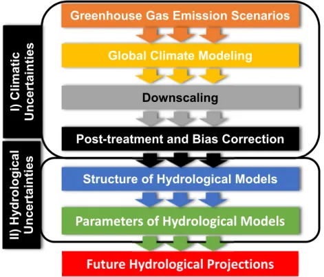
Hydrological simulations under climate change are subject to both conventional modelling uncertainties in stationary climate as well as those related to work with future climate scenarios. These uncertainties are compared in literature to a cascade. In a simplified way, it may be divided into two parts: climatic uncertainties and hydrological uncertainties. Figure 1 schematizes these
uncertainties as well as the methods used to lead to the production of hydrological projections. The different phases used in these potential ways are detailed in the sections below: Greenhouse Gas Emission Scenarios; Global climate modelling; Downscaling; Post-treatment and bias correction; Hydrological projections.
Figure 1 - Schematic view of the cascading uncertainties that are subject to the hydrological projections in the context of climate change.
1.1.1. Climatic uncertainties
1.1.1.1. Greenhouse Gas Emission Scenarios
The Greenhouse Gas Emission Scenarios (Step 1) correspond to a probable representation of the future climate based on a coherent and a homogeneous ensemble (Parry and Carter, 1998; Parry, 2002). These scenarios are generally intended to serve as inputs for the study of the anthropogenic climate change impact (IPCC, 2001). They are determined mostly by the IPCC
Greenhouse Gas Emission Scenarios
I) Climat ic Uncertainties II) Hy drological Uncertainties
Global Climate Modeling
Downscaling
Structure of Hydrological Models
Parameters of Hydrological Models
Future Hydrological Projections
Post-treatment and Bias Correction(Intergovernmental Panel on Climate Change), mainly in the SRES report (Special Report Emissions Scenarios, IPCC: (Nakićenović et al., 2000).
The different families of scenarios are based on various future world foundations, especially in terms of population (demography), economy, technology, energy and land use. Figure 2 illustrates families of scenarios and their main aspirations: a world oriented towards the economy or to the environment, with a regional operation or rather global coverage.
Figure 2 - Schematic representation of the four main families of SRES scenarios (Source: IPCC: (Nakićenović et al., 2000)).
A1 scenarios describe a future world with very rapid economic growth, low population growth, and rapid introduction to new and more efficient technology. It relies on the convergence between regions, strengthening of cultural and social interactions, and substantial reduction of regional disparity in per capita income.
A2 scenarios are founded on a very heterogeneous world, which is based on self-sufficiency and preservation of local identities. It integrates a continuous increase of the population (regional fertility rates converge very slowly) and an economic development of the regions. The per capita economic growth and the technological advances are fragmented.
B1 scenarios describe a future world with the same demographic conditions as A1, but with rapid changes in the economic structures toward a service and information economy. It is also oriented towards the establishment of clean technologies with efficient use of resources and activities that produce less waste. It focuses finally on the importance of a global solution for economic, social, and environmental viability, with greater equity, but without additional climate initiatives.
B2 scenarios present a future world with more local solutions to economic, social, and environmental challenges. The world population increases regularly, the economic development is intermediate and the technological advances are slower and more diverse than for A1 and B1. This scenario also focuses on environmental protection and social equity with local and regional approach. The IPCC recommends the use of the A2 emission scenario (high emission of greenhouse gases) and B2 (medium to low emission) for intercomparison studies (Nakićenović et al., 2000).
It is important to note that these scenarios represent the first level of uncertainties. They are mainly based on economic and sociological considerations, but also on natural evolution. Indeed, all scenarios make assumptions about the demographic trends, energy demand, land use, and greenhouse gas emissions (Prudhomme et al., 2003).
More recently, emission scenarios have evolved toward greenhouse gas concentrations instead of greenhouse gas emissions. Indeed, the most recent works by the IPCC are based on RCPs (Representative Concentration Pathways, (Van Vuuren et al., 2011)) that target different levels of forcing. They enable the
consideration of climate policy to reduce greenhouse gases, as well as greater flexibility in the use: in-depth assessment and retrospective forecasts (Moss et
al., 2010).
Therefore, these scenarios are used to drive global atmospheric circulation models, which generally describe the same process, but with various representations of the processes, different spatial and temporal scales, and so forth. They may also differ in the parameterization of dynamic phenomena and in the definition of the initial state of the climate system.
1.1.1.2. Global climate modelling
Global climate modelling (step 2) is based on the use of Global Climate Models (GCMs), which are currently the most reliable tools to simulate the response to the rise of greenhouse gas concentrations. They estimate the changes in the climatic variables (temperature, precipitation, radiative flows, vapor pressure, wind speed, and others) for the entire planet (Prudhomme et al., 2003; Plummer
et al., 2006), based on mathematical representations of the physical processes
related to the atmosphere, oceans, icecaps, and Earth surface (IPCC, 2001). Many Global Climate Models have been developed and it is assumed that none of them provides better results. It is important to note that they do not provide future climate forecasts but climatic evolution projections based on scenarios. Their spatial resolution is about 300 km.
The chaotic nature of the weather limits meteorological forecasts to 15 to 30 days, but maintaining water and energy balances GCMs are devised to simulate climate over much longer periods and are able to account for changes in greenhouse gas concentrations.
Climate modelling may also resort to an “Ensemble Approach”, by providing several simulations (called "members") generated by running the same GCM many times with slightly different initial conditions or by introducing slight perturbations to the modelling system. This approach allows for the estimation of
the uncertainty associated with the internal variability of the climatic models, i.e. the natural variability of the climate. These simulations are considered “equiprobable” even if they produce different realisations in time and space.
The comparison between the various members allows an assessment of the incompressible uncertainties due to the representation of the climate variability (chaotic system). Also, within the framework of the study on the extremes, the use of climate members allows an extension of the data sample, thus adding robustness to the analysis.
For these various reasons, it is understandable that many uncertainties, due to physical, digital (“structural”), and climate natural variability, are associated with their use.
The importance of the uncertainties associated to the global circulation models is substantial. Covey et al. (2003) show that none of the 18 circulation models tested in their study reproduces observations.
To carry out studies at regional scale, the data resulting from global models should be disaggregated. Once again, there exist various methods of downscaling. First, dynamic approaches that consist of simulations on the regional scale of climatic dynamics by applying regional models of circulation. Second, statistical (empirical) approaches that build links between climate state on large scale and the characteristics of the local climate, such as weathers types’ method.
Therefore, the climate data genesis processes on a regional scale is subject to a supplemental set of uncertainties. The quantification of these errors is generally carried out by studying the dispersion of the outputs associated with the use of each emission scenario, global circulation models, and downscaling methods. These uncertainties are climatic and influence strongly the hydrological modelling since they concern the input data for hydrological models (precipitation and temperature in particular).
1.1.1.3. Downscaling techniques
a) Dynamical downscaling
Dynamical downscaling consists in building a Regional Climate Model (RCM) at a finer spatial scale (about 25 km, even less), which makes use of the GCM values for boundary conditions.
The main advantage of this methodology is to physically represent the processes influencing the climate (because forced by the GCM); its disadvantages include high computing times and the fact that the bias associated with the climatic variables of the GCM is transmitted to the RCM (Kay et al., 2006; Fowler and Kilsby, 2007; Stendel et al., 2007; Minville et al., 2008; Lavender and Walsh, 2011; Pierce et al., 2013; Pinto et al., 2014; Maraun et al., 2015; Ohba et al., 2015).
b) Statistical downscaling
Statistical downscaling seeks a transfer functions between large-scale climate variables (GCM) and local ones. These transfer functions are then used to downscale the GCM for the future climate conditions. This stochastic approach is quite sensitive to the choice of variables, domains, periods of calibration, seasons, etc. Moreover, it makes the simplifying assumption that the transfer functions remain valid for the future climates (Landman et al., 2001; Wilby et al., 2004; Diaz-Nieto and Wilby, 2005; Chu et al., 2010; Jakob Themeßl et al., 2011; Themeßl et al., 2012; Simon, 2014; Dayon et al., 2015).
c) Other methodologies
Other methodologies of downscaling can also be mentioned:
(1) Weather Typing (WT) associates the weather classes to climatic variables and allows for the future climate simulations to involve the same types of weather variables subject to climate change (IPCC, 2001);
(2) Weather Generator (WG) is devised to produce random sequences of weather variables consistent with an observed climate. Their parameters may be adjusted to simulate future conditions (Semenov and Stratonovitch, 2010);
(3) Analogous Method (AM) compares simulated atmospheric states with observed ones (history), then the most similar atmospheric condition is resampled (Zorita and Von Storch, 1999);
(4) Statistics on the model outputs can be developed following the delta method (Minville et al., 2006) or the Quantile Mapping method (Hahn and McQuigg, 1970; Boé et al., 2007; Salathe et al., 2007).
These last approaches of downscaling, and in particular the statistics on the outputs, are often applied to the RCM, i.e. to the outputs of a dynamical downscaling. Indeed, the downscale of a RCM is still not well adapted to the objectives of the application of climatic data.
1.1.1.4. Post-treatment and bias correction
For a given period of observed data (called reference or control period) the comparison between the RCM results (in general) and the meteorological observations often highlights a bias in the results. From a hydrological perspective this bias is particularly sensitive for temperature and precipitation (intensity and frequency).
Bias correction is thus a procedure that seeks to adjust the simulated future data from observations for the control period (Minville et al., 2009; Hurkmans et al., 2010; Hirschi et al., 2011; Kriauciuniene et al., 2012; Stojanović et al., 2013; Brigode et al., 2014; Mahoney et al., 2015). The concept consists in identifying a bias between the observations and the model outputs (especially for the variables of interest), then finding parameters of “correction” in order to adjust the model outputs. The methodology then assumes that the bias related to the period of control will be the same in the future (Wood et al., 2004; Minville et al., 2009; Bring and Destouni, 2011; Bürger et al., 2012; Werner et al., 2013; Schnorbus et
This procedure can address the spatial and the temporal scale of the data. Many studies have used this method on the minimum and the maximum temperatures (Wood et al., 2004; Fowler et al., 2007; Fowler and Kilsby, 2007; Minville et al., 2009; Bordoy and Burlando, 2013; Livneh et al., 2013; Wang and Chen, 2014; Rust et al., 2015) and on the frequencies and intensities of precipitation (monthly mean) for e.g. the Local intensity Scaling method (Schmidli et al., 2006; Rossa et
al., 2008; Tao and Barros, 2010; Hagemann et al., 2011; Jeong et al., 2013; Gao et al., 2014; Velázquez et al., 2015).
Downscaling techniques (dynamic and / or statistical) and bias correction must be seen as tools to attain a better representation of the local climatic conditions from global and regional models (Wood et al., 2004).
1.1.2. Hydrological uncertainties
The lower part of the cascade of Figure 1 includes all uncertainties in the application of hydrological models, which is subject to many uncertainties involved at different levels of the modelling process:
1.1.2.1. The input data for hydrological models
The observations used as input data for models: typically information on precipitation and temperature (potential evapotranspiration, e.g. Oudin et al. (2006)) and calibration/validation data (typically information on streamflows, e.g. (Ibbitt (1972); Kavetski et al., 2006)), which are primary sources of errors.
1.1.2.2. The structure of hydrological models
The structure of a model comes from general assumptions on the rainfall-runoff relationship (Mathevet, 2005), i.e. equations and concepts describing the many physical processes. In the context of climate change, certain processes or assumptions that are not taken fully into account may become non-negligible and thus induce potential errors. The estimation of these errors is often approached by comparing outputs from many models (Wilby, 2005; Seiller et al., 2012).
1.1.2.3. The parameters of distributed or lumped hydrological models
These parameters are generally not measurable physical variables; indeed they require a calibration phase of the model. The calibration procedure, the choice of data used for these phases, the objective function considered, the parameter equifinality (different parameter sets that induce comparable performance) generate errors in the identification of the model parameters. In the context of non-stationary climate, this identification can become more uncertain when physical changes of the watershed are not taken into account (change in vegetation cover for example). These potential errors are widely recognized by the scientific community, but their impacts on hydrological projections in the context of climate change have been sparsely studied (Beven and Binley, 1992; Vrugt et al., 2003; Jin et al., 2010; Najafi et al., 2011; Shen et al., 2012; Brigode
et al., 2013; Wanders et al., 2014; Fan et al., 2015; Haque et al., 2015;
1.1.3. Quantification of these two sources of uncertainties
The sources of uncertainties that have been highlighted previously interact with each other (the model structure plays on the parameter values; the inputs also influence the parameters during the calibration procedure), which makes their quantification more difficult. There are quite some studies ranking the many error sources in the context of non-stationary climate:
The study performed by Wilby and Harris (2006) of two rainfall-runoff models on a watershed located in England allowed considering the structure of the global circulation models as the most important source of uncertainty, followed by the (empirical) downscaling method, the hydrological model structure, the hydrological model parameters, and finally the emission scenario. Kay et al. (2006) carried out a similar study on two other British catchments and also ranked the structure of the global circulation models as the main source of error, but found the emission scenarios more uncertain than the hydrological modelling. The results of the project RExHySS (Ducharne et al., 2010) also showcase the highest significance of errors due to Global Circulation Models (GCMs) compared to hydrological modelling uncertainties.
Finally, in a general study aiming to compare several sources of uncertainty in the context of climate change, Kay et al. (2009) quantified the impact of parameter uncertainty. A robust statistical test was set up: each constituent year of the time series is alternately "forgotten" during the calibration phase that generates, for a time series of n years, n + 1 different parameter sets. Their results showed that this uncertainty has a lower impact than the other considered error sources (GCMs, downscaling methods). However, the authors note that equifinality, which is not considered in their study, could have a strong impact on the uncertainty in the model parameters.
Uncertainties related to the use of hydrological models under climate change seem to be considered "non-dominant" compared to those related to the climate
projections. However, prior experiments were usually unbalanced: dozens of future scenarios, of global circulation models or of downscaling methods can be selected and tested on only one or two hydrological models; Still Wilby (2005) noted that depending on the rainfall-runoff model used (and possibly the catchment studied), the uncertainties associated with hydrological modelling may predominate. Also, it seems important to note that these rankings were obtained on a limited number of watersheds. Blöschl and Montanari (2010) noted in fact that the detection of very large uncertainties in a watershed is difficult to generalize to a region.
More recently, Chen et al. (2011) showed, on a Canadian catchment, that the choices of GCMs and downscaling techniques are the greatest uncertainty sources in hydrological projection estimations, followed by greenhouse gas emission scenarios and hydrological model structures, and lastly hydrological model parameter estimation. Focusing on future hydrological trends in the UK, Arnell (2011) showed that “uncertainty in response between climate model patterns is considerably greater than the range due to uncertainty in hydrological model parameterization”.
On several southeastern Australian catchments, Teng et al. (2012) also showed that uncertainties stemming from fifteen GCM outputs are much greater than the uncertainties stemming from five hydrological models. These results show that the uncertainties generated by the hydrological modelling step, though generally lower than that generated by the climate modelling step, can be important in some cases and should not be ignored in climate change impact studies.
1.2. Uncertainties related to the parameters of the
hydrological models
The errors related to the parameters of the hydrological models in the context of climate change are induced by the non-robustness of the parameter identification
procedure (Kavetski et al., 2011; Brigode et al., 2013; Gharari et al., 2013) as well as the parameter sets equifinality. While few studies deal with the problem of parameter robustness, the issues of equifinality have been studied for several years by the hydrological community (Beven and Binley, 1992; Franks et al., 1997; Beven and Freer, 2001; Beven, 2006; Vrugt et al., 2009; Beven et al., 2012; Beven and Young, 2013; Ficklin and Barnhart, 2014; Her and Chaubey, 2015). Many standard methods exist to quantify the impact of equifinality on hydrological simulations. Nevertheless, it seems that these methods are mostly tested in a stationary climate condition. Similarly, the consideration of the non-robustness of the parameter identification and the equifinality of parameter sets as two sources of error is usually set up for non-changing climates.
1.2.1. Robustness of the parameter identification
1.2.1.1. Sensitivity of the parameters to the calibration period
Several general studies aimed to investigate the parameters’ sensitivity to the calibration period. These tests were usually performed in stationary climate conditions, due to the limited length of the time series. Climatic contrasts were then obtained by considering particular hydro-climatic sub-periods, which created the required non-stationary context:
Gan and Burges (1990) used the SACRAMENTO model on five small hypothetical watersheds, i.e. with homogeneous flat surfaces. The authors showed that the parameter values are dependent on hydro-climatic properties of the period used to calibrate the model. Thus, these conclusions must be taken into account especially when working in the context of climate change.
Jakeman et al. (1993) tested the IHACRES model on two watersheds (North Carolina and Wales) and 10 periods of calibration (of 2 to 3 years of length) previously identified in the observed data. These different sets of parameters were then tested in a non-stationary climate context (increase in the average temperature of the air from 1 to 3° C). Simulations with these different sets of
parameters were similar, which prompted the authors to conclude on the possibility of using the IHACRES model with non-stationary weather.
Wilby (2005) experimented with two versions of the CATCHMOD model on the Thames watershed. The observed data was first used as calibration period of the model. Two particular hydrological years were then considered: Dry (1975-1976) and Humid (1967-1968). The stability of the parameters and the dispersion of the outputs were different depending on the model structure: the simplest model (i.e. with the fewest parameters) presented a high variability of parameter values, while the most complex structure (i.e. with the most parameters) implied greater stability of the parameter values.
1.2.1.2. Temporal stability of "optimal" parameter values
Other studies focused on the hypothesis of temporal stability of optimal parameters:
Wagener et al. (2003) studied the evolution of the optimal parameters with time, for a rainfall-runoff model applied on a single reservoir watershed of 1256 km², located in south-east England. For that, Dynamic Identifiability Analysis (DYNIA) developed by Wagener et al. (2001) was used. It allows to highlight the temporal instability of the distribution of optimal parameters and the uncertainty related to these parameters. First, it requires the implementation of Monte Carlo simulations. The instability is evaluated over a rolling period, fixed length, browsing the entire observed time series. The results of this study highlighted a substantial temporal variation of the optimal parameters.
Choi and Beven (2007) came to the same general conclusion by applying the GLUE method with the TOPMODEL model on a 150 km² watershed located in South Korea. This study consisted in dividing the observed chronic in periods that are hydrologically similar. These results also showed that parameters vary considerably on all 15 identified hydrological periods.
van Werkhoven et al. (2008) quantified the sensitivity of the parameters of the SAC-SMA model with the hydro-climatic characteristics of the input data. This study was carried out on 12 watersheds located throughout the United States and thus marked by different climates. In particular, the results showed some variations of the sensitivity of the parameters related to changes of the hydro-climatic conditions of entries of the model.
Abebe et al. (2010) also analyzed the temporal change of the optimal parameter values of the HBV model through the DYNamic Identifiability Analysis (DYNIA) approach. 60,000 Monte Carlo simulations were carried out on a watershed of 1,944 km² located in the state of Mississippi and having a time series of 40 years of data. A discretization of the time series was performed to quantify the error made at each time step. The results showed that the identification of optimal parameters was easier on certain periods and that these optimal values varied over time.
Finally, De Vos et al. (2010) proposed to use these conclusions to improve hydrological model calibration procedures by considering the model parameters as time-varying. The proposed optimization procedure was tested with the HyMod model (with 5 free parameters) on the same watershed used in the study of Abebe et al. (2010). The observed data were divided into 12 hydrologically similar periods to which 12 optimal parameter values were associated. Thus, these optima were considered as evolving in time in order to compensate the errors of the model structure identified previously. Different structures of the HyMod model were tested while being fixed in three distinct ways: two calibrations with non-varying parameters and one dynamic calibration with parameters that can vary over time. The latter procedure induced better performance of the model.
The whole of these articles tend to show the temporal instability of the optimal parameter values of the hydrological models, which reveals the errors in the structure of the models. Thus, the definition of an optimal parameter set for a given time series data seems more dubious than the consideration of several
optimal parameter sets. This strong assumption is primarily due to the errors of the hydrological models structure.
1.2.1.3. Stability of the parameters in non-stationary observed conditions
Non-stationary conditions, particularly in West Africa, were used to assess the stability of the parameters of hydrological models. Indeed, for several decades, a marked decrease in rainfall has been observed since 1970 in this region. These studies are particularly valuable because they help to better understand the problem of identification of the hydrological model parameters in the context of a changing climate.
Niel et al. (2003) worked on a sample of 17 watersheds located in West and Central Africa. These basins of various surfaces were modelled through the GR2M model. For each basin, the model was calibrated on two different sub-periods: one before the change of the early 1970s and one thereafter. Results show that the stability of parameters depends on the considered watershed itself, but also that a strong dispersion of the parameter values was not necessarily related to the climate variability.
Le Lay et al. (2007) tested the GR4J model on the Benin basin (10 050 km ²), which is concerned by the existence of climatic contrasted periods: a “wet” period (1954-1970) followed by a “dry” one (1972-1990). These two segments as well as the whole of the chronic were used for the calibration of the model. A random sampling of the years was then carried out in order to obtain 100 sets of optimal parameters. Then, the dispersion of these parameters was compared with those obtained with the calibration carried out over the dry period and the wet period. These dispersions being of the same order of magnitude, the authors conclude as for a relative stability of the parameters values in non-stationary observed conditions.
The results of these two experiments, based on conditions of non-stationary climate, indicate that a climatic variation is not obligatorily accompanied by an increased instability of the parameters values of the considered models.
1.2.2. The concept of equifinality and the Generalized Likelihood
Uncertainty Estimate (GLUE) method
The equifinality of the hydrological model parameters is a problem largely recognized by the scientific community: there exists a significant number of standard methods to quantify the uncertainty related to the equifinality of the parameters sets, notably the Metropolis Monte Carlo method (Metropolis et al., 1953; Kirkpatrick et al., 1983) and the Regional Sensitivity Analysis method (Johnston and Pilgrim, 1976; Hornberger et al., 1985; Duan et al., 1992; Beven, 1993; Kuczera, 1997; Gupta et al., 1999).
The most used method in literature is GLUE: Generalised Likelihood Uncertainty Estimate of Beven and Binley (1992). It is built around this fundamental limit of hydrological models which is the equifinality of the parameter sets, i.e. and the absence of a single optimal parameter set. Thus, a less uncertain hydrological projection would be a combination of various parameter sets which are weighted by a probability distribution of these parameter sets. This priori probability distribution is considered to be the likelihood of the model and therefore allows to accept or reject some simulations by defining a probability threshold. This approach allows estimating the uncertainty in the parameter sets’ equifinality. Freer et al. (1996) show that the quantification is strongly influenced by the choice of the probability distribution of the parameter sets.
There are various possible uses of the general methodology of GLUE:
The exploration of the parameter space: The genesis of a large number of random parameters can be realized through different sampling methods. Monte Carlo (Metropolis and Ulam, 1949) provides a random visit of the parameter space. The Latin Hypercube method, which consists in dividing the space of the parameters into subsets, forces a draw in each of these sub-assemblies and allows a general review of possible parameters sets. This latter technique allows a more thorough exploration of the parameters space and requires less computing time. Parameters optimization techniques may also be used. The Shuffled Complex
Evolution-UA (SCE-UA (Duan et al., 1992), developed in order to identify the optimal parameter set, consists of a preliminary sampling of the Latin Hypercube type, which then tends to converge towards an optimal parameter set.
The acceptability threshold of parameter sets: The generated parameter sets must be tested in order to characterize their acceptability. There exist two simple ways to determine this threshold. First, it is possible to fix the number of parameter sets to be retained. The threshold can also be defined according to a maximum value of the considered objective function, obtained after a preliminary model calibration. Then the threshold of acceptability of a parameter set corresponds to a certain percentage of this maximum value. Other more complex methods are possible as well (Alazzy et al., 2015).
GLUE type approaches add a weight to each acceptable parameter set: certain of them are regarded as closer to the optimal parameters set than others. This relative weight of the parameters set is allotted through a likelihood function. Therefore, the quantification of uncertainties related to the equifinality requires the establishment of a sampling of the parameter space. Then, all generated parameter sets are to be tested with the considered model. An arbitrary threshold is then fixed in order to reject certain parameter sets. The definition of this threshold is not explicit in most of the studied methodologies.
1.3. Research objectives
Previous studies related to hydro-meteorological modelling in a context of climate change and lessons learned from prior experimentations lead us to propose this project that aims to reinforce knowledge on this subject, to combine different sources of hydrological uncertainties, especially those related to parameter identification, equifinality and use of different structures for hydrological modelling, and to explore novel research orientations. Thus, the purpose of this section is to detail the three objectives which were identified: