3D numerical simulation of a lab-scale pressurized dense fluidized bed focussing on the effect of the particle-particle restitution coefficient and particle–wall boundary conditions

Open Archive TOULOUSE Archive Ouverte (OATAO)

OATAO is an open access repository that collects the work of Toulouse researchers and

makes it freely available over the web where possible.

This is an author-deposited version published in :

http://oatao.univ-toulouse.fr/

Eprints ID : 15726

To link to this article :

DOI:10.1016/j.ces.2015.11.016

URL : http://dx.doi.org/10.1016/j.ces.2015.11.016

To cite this version :

Fede, Pascal and Simonin, Olivier and Ingram, Andrew 3D

numerical simulation of a lab-scale pressurized dense fluidized bed

focussing on the effect of the particle-particle restitution coefficient

and particle–wall boundary conditions. (2016) Chemical

Engineering Science, vol. 142. pp. 215-235. ISSN 0009-2509

Any correspondence concerning this service should be sent to the repository

administrator: staff-oatao@listes-diff.inp-toulouse.fr

3D numerical simulation of a lab-scale pressurized dense fluidized bed

focussing on the effect of the particle-particle restitution coefficient

and particle–wall boundary conditions

Pascal Fede

a,b,n

_{, Olivier Simonin}

a,b

_{, Andrew Ingram}

c

a_{Université de Toulouse; INPT, UPS; Institut de Mécanique des Fluides de Toulouse Allée Camille Soula, FR-31400 Toulouse, France} b_{CNRS; IMFT; FR-31400 Toulouse, France}

c_{School of Chemical Engineering; University of Birmingham; Birmingham, UK}

H I G H L I G H T S

! Comparison between time-averaged Euler particle velocity profiles and PEPT results.

! Prediction of double toroidal recir-culation loops for large solid wall shear stress.

! Testing of No-slip wall boundary condition for Euler particle velocity.

G R A P H I C A L A B S T R A C T

Keywords: Gas-solid flows Dense fluidized bed CFD

Wall boundary conditions PEPT

a b s t r a c t

3D numerical simulations of dense pressurized fluidized bed are presented. The numerical prediction of the mean vertical solid velocity are compared with experimental data obtained from Positron Emission Particle Tracking. The results show that in the core of the reactor the numerical simulations are in accordance with the experimental data. The time-averaged particle velocity field exhibits a large-scale toroidal (donut shape) circulation loop. Two families of boundary conditions for the solid phase are used: rough wall boundary conditions (Johnson and Jackson, 1987 and No-slip) and smooth wall boundary conditions (Sakiz and Simonin, 1999and Free-slip). Rough wall boundary conditions may lead to larger values of bed height with flat smooth wall boundary conditions and are in better agreement with the experimental data in the near-wall region. No-slip or Johnson and Jackson's wall boundary conditions, with sufficiently large value of the specularity coefficient ðϕZ0:1Þ, lead to two counter rotating mac-roscopic toroidal loops whereas with smooth wall boundary conditions only one large macmac-roscopic loop is observed. The effect of the particle-particle restitution coefficient on the dynamic behaviour of flui-dized bed is analysed. Decreasing the restitution coefficient tends to increase the formation of bubbles and, consequently, to reduce the bed expansion.

1. Introduction

Pressurized gas–solid fluidized beds are used in a wide range of industrial applications such as coal combustion, catalytic poly-merization, uranium fluoration and biomass pyrolysis. The math-ematical modelling and numerical simulation of such industrial fluidized beds are challenging because many complex phenomena http://dx.doi.org/10.1016/j.ces.2015.11.016

n_{Corresponding author at: Université de Toulouse; INPT, UPS; Institut de}

Mécanique des Fluides de Toulouse Allée Camille Soula, FR-31400 Toulouse, France E-mail address:pascal.fede@imft.fr(P. Fede).

are in competition (particle–turbulence interaction, particle–par-ticle and parparticle–par-ticle–wall collisions, heat and mass transfers) and because of the large-scale geometry of the industrial facilities compared to the characteristic length scales of the fluid and particles.

The development of numerical modelling of dense fluidized bed hydrodynamics started about three decades ago (Gidaspow, 1994). Basically two approaches can be used for the numerical prediction of dense fluidized bed hydrodynamic: the Euler-Lagrange approach, where filtered Navier–Stokes equations are solved for the gas and Discrete Element Method (DEM) for the particles (Kaneko et al., 1999;Deen et al., 2007;DiRenzo and Di Maio, 2007;Olaofe et al., 2014), or the multi–fluid approach where all phases are treated as continuum media. In the DEM approach, the Lagrangian trajectories of each particle are computed and the inter–particle collisions are treated in a deterministic manner. Even if DEM can be used up to a few millions of particles (

Cape-celatro and Desjardins, 2013) it cannot yet be used for most of

industrial full-scale simulations. Typically, to simulate the lab-scale fluidized bed studied in the present paper, the whole number of particles to be accounted for in the frame of the DEM approach is about 10 millions while for an industrial pressurized gas-phase olefin polymerization reactor (Neau et al., 2013) the corresponding number of particles should be larger than 40 billions. In contrast, nowadays it is possible to perform realistic 3D simulations of industrial configurations by using an unsteady Eulerian reactive multi-fluid approach. Numerical simulations of industrial-, pilot-and lab-scale pressurized reactors were carried out with such an approach showing a good agreement with the qualitative knowl-edge of the process but detailed experimental validations were missing (Gobin et al., 2003;Fede et al., 2010;Rokkam et al., 2010;

Fede et al., 2011a,2011b;Rokkam et al., 2013). Indeed, the Euler– Euler approach is extensively used for circulating or dense gas-solid fluidized bed predictions but the model assessment is com-monly restricted to a comparison between the predicted and the experimentally measured pressure drop, or local mass flux. Obviously such restrictions come from the complexity of doing measurements inside a dense particulate phase. Recently, an ori-ginal experimental technique, called Positron Emission Particle Tracking (PEPT), has emerged allowing to measure the trajectory of an individual particle moving in dense particulate flows. From the trajectory it is possible to compute the particle dispersion properties and then to perform fruitful comparison between experiments and numerical prediction (Link et al., 2008;Fede et al., 2009).

The present paper shows numerical results from Euler–Euler simulations carried out with the mathematical model proposed by

Balzer et al. (1995)(seeAppendix A). Such a modelling approach

involves several assumptions however there is no empirical con-stant in the model. In fact the model, like all Lagrangian or Eulerian ones, requires the value of the normal restitution coeffi-cient for particle-particle collision. Precisely speaking, the normal restitution coefficient is not an adjustable parameter because it represents the physical loss of kinetic energy during a collision. However, as this parameter is very difficult to measure for a practical powder (Foerster et al., 1994; Sommerfeld and Huber, 1999), it can be seen as a parameter of the modelling approach

(Goldschmidt et al., 2001). In the present paper a comprehensive

analysis is made for showing how the normal restitution coeffi-cient may modify the macroscopic properties of a dense fluidized bed.

In the framework of the kinetic theory of dry granular flows, several wall boundary conditions for the solid phase have been derived for rough or flat walls, with or without frictional effect (Hui et al., 1984;Johnson and Jackson, 1987;Jenkins and Richman, 1986;Jenkins, 1992;Jenkins and Louge, 1997;Sakiz and Simonin,

1999;Konan et al., 2006b;Schneiderbauer et al., 2012;Soleimani et al., 2015). For the numerical simulation of a circulating or dense fluidized bed the most popular wall boundary conditions are the ones derived byJohnson and Jackson (1987)which introduced a specularity coefficient that is an ad-hoc parameter depending on the large-scale roughness of the walls but which cannot be mea-sured directly from experiment, in contrast to the normal resti-tution coefficient (Sommerfeld and Huber, 1999). In the case of dilute gas-solid flow in a pipe,Benyahia et al. (2005)showed that the specularity coefficient must be very small for correct agree-ment with experiagree-mental data.Li et al. (2010)analysed the effect of the specularity coefficient on the predicted 2D and 3D hydro-dynamic of dense bubbling fluidized beds. Unfortunately, the 3D study considered only small values of the specularity coefficient ranging from 0.0 to 0.05. In parallel, wall boundary conditions have been derived for flat frictional walls (Jenkins and Richman, 1986;Jenkins, 1992;Louge, 1994;Jenkins and Louge, 1997;Sakiz

and Simonin, 1999;Schneiderbauer et al., 2012). The development

and validation of such boundary conditions were mainly per-formed by comparison with predictions from the Discrete Element Method (DEM).

It is important to note that the original Johnson and Jackson boundary conditions do not account for particle/wall frictional effects. In contrast, the more recent boundary conditions ofKonan et al. (2006a, 2006b) andSoleimani et al. (2015)extend different approaches, originally developed for smooth walls, by using the idea of virtual wall angle ofSommerfeld and Huber (1999).

The paper is organized as follows. The second section gives an overview of the experiment where the PEPT technique was used for obtaining local statistics of the solid inside the fluidized bed. The boundary conditions for the solid phase employed in the present study are described in the third section. The description of the numerical simulation, in terms of equations, mesh, material properties and statistics are given in the fourth section. The results are presented in section five and, finally, an analysis is carried out in section six on the specific dependence of the simulation results on the particle-particle collision restitution coefficient and on the solid wall boundary conditions. Conclusions and prospects are given in the last section.

2. Experimental overview

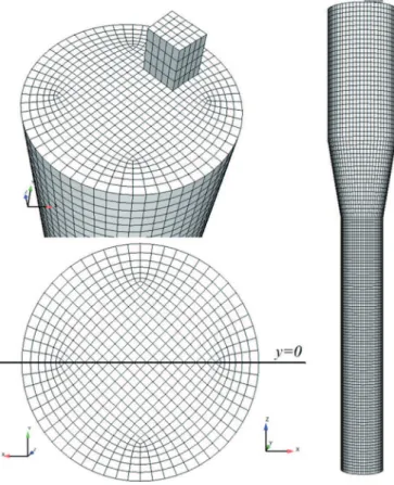
This study concerns the hydrodynamics of an isothermal gas-solid dense fluidized bed in a low-scale pressurized axisymmetric reactor with a cylindrical column of internal radius R ¼ 77 mm and height 1 074 mm (see Fig. 1). The vertical distance between the horizontal gas fluidization distributor plate and the widening (with an enlargement half-angle of 10°) is 924 mm. Nitrogen enters at the distribution plate with a fluidization velocity Vf¼

0:32 m=s and the pressure in the fluidized bed is 12 bar. The gas and solid material properties are given in Table 1. The particle phase is almost monodisperse with a median diameter of 875

μ

m and a material density of 740 kg=m3_.

Positron Emission Particle Tracking (PEPT) is an experimental technique developed at the University of Birmingham derived from the medical imaging method Positron Emission Tomography (PET) (Stellema et al., 1998). PEPT enables the tracking of a single particle in an opaque or otherwise impenetrable system such as dense fluidized beds. PEPT tracers are labelled with a specific class of radioisotope which decays through the emission of a positron (

β

þ _{decay). The emitted positron collides with a local electron,}

annihilates and produces a pair of back-to-back gamma photons. The usual isotope is Fluorine-18; this has excellent characteristics of decaying solely through

β

þ_{, is easily manufactured by Helium-3}

silica, and has a half-life of about 2 hours giving a good balance between activity and tracer life (4–6 h). Tracers will have decayed by a factor greater than 4000 within 24 hours so there is no concern for equipment contamination.

Adapted PET cameras are used to detect the photon pairs and generate the so-called Lines Of Responses (LORs) that connect each pair. Triangulation of successive LORs should give the point in space where the annihilation occurred - the tracer location. In practice there is some corruption of data due to a mixture of Compton scattering of photons and incorrect pairing. The

algorithm developed at Birmingham over many years (Ingram et

al., 2007a) eliminates corrupted data thorough a statistical

pro-cedure; typically aliquots of 200–500 LORs will be used to com-pute the tracer location to within 0.5–1.0 mm at a frequency between 100 and 1000 Hz. The reliability and frequency of loca-tion depends on many factors such as tracer activity, tracer velo-city, size of rig and mass of material to be penetrated by the photons.

Historically, the PEPT facility has progressed from the home-made multiwire positron camera in 1984, through the ADAC Forte Medical PET camera in 1999 (giving a 20–fold increase in data frequency) to more recent developments of the flexible, modular PEPT system built from the components of redundant PET scan-ners.This latter development has enabled exploitation of the technique for larger and/or more complicated geometries (Ingram et al., 2007b).

During the experimental data acquisition Neparticle positions

have been recorded. The time–averaged Eulerian solid velocity, volume–averaged in a cell CðxÞ, centred at x, is defined by UpðxÞ ¼ PNe k ¼ 1 upðtkÞ

Δ

tk

δ

k PNe k ¼ 1

Δ

t_k

δ

k with

δ

k¼ 1 if xpðtkÞACðxÞ 0 otherwise " ð1Þ

where xpðtkÞ is the instantaneous particle position at the time tk.

Link et al. (2008)proposed the following expression for the

time-averaged Eulerian solid velocity

UpðxÞ ¼ PNe k ¼ 1 upðtkÞ

δ

k PNe k ¼ 1

δ

k : ð2Þ

These equations give the same result when

Δ

t is uniform so the difference in weighting is not related to the time spent in the cell, rather the activity of the tracer at the time it passes through. At the start of the experiment, the tracer is strong so will be seen more frequently and Eq.(2), being a count average of observed velo-cities, would unfairly weight in favor of early data. Eq. (1) is effectively averaging according to distance traveled through the cell so will be unaffected by tracer activity. Actually for a given data frequency, slow particles will be observed more times (and vice-versa for rapid particle) so both expressions weight according to time spent in the cell and will give more emphasis to the slower particles. This analysis remains valid if the data frequency is varying but not correlated with the instantaneous particle velocity, meaning that the tracer activity and the sensor system is unaf-fected by the particle motion. In the following, even if we did not find significant differences between the two definitions, Eq.(1)is used to compute the time-averaged Eulerian solid velocity in a cell because this definition is more consistent with the one of the time-averaged Eulerian solid velocity in the frame of the statistical approach.

It must be noticed that the accuracy of the time–averaged Eulerian solid velocity defined by either Eqs.(1)or(2) depends on the cell size. Indeed, if the number of events in a cell is too small, the computed Eulerian solid velocity becomes unrepresentative. Conversely, if the cell is too large, the number of events is large enough with respect to the statistical averaging but the spatial accuracy of the local information is lost due to spatial averaging (Fede et al., 2009). But, owing to the axisymmetry of the reactor geometry, the time-averaged flow may be assumed to obey cylindrical symmetry. So, the spatial averaging of the time-averaged variables can be performed in the azimuthal direction without loss of accuracy. Consequently, the effective

volume-Fig. 1. Geometry of the low–scale fluidized bed. Table 1

Gas and particle material properties given for the operating conditions Pg¼ 12 bar

and T ¼ 298 K.

Nitrogen Density, ρg [kg/m3] 13.595

Viscosity, μg [Pa.s] 1:7982 & 10' 5

Fluidization velocity, Vf [m/s] 0.32

Particles Density, ρp [kg/m3] 740

Mean diameter, dp [μ m] 875

averaging cell CðrÞ, in Eqs.(1) and (2), is a cylindrical ring, of radius r, centered on the symmetry axis.

3. Wall boundary conditions

The Euler-Euler modelling approach is a hybrid two-fluid approach (Morioka and Nakajima, 1987) where separate trans-port equations (mass, momentum, and fluctuating kinetic energy) are solved for each phase and coupled through interphase transfer terms. The transport equations are derived by phase ensemble averaging weighted by the gas density for the continuous phase and by using kinetic theory of granular flows supplemented by fluid effects for the dispersed phase (Balzer et al., 1995). In the present study the gas flow is considered as laminar and, for the solid phase stress tensor modeling, a viscosity assumption is used

(Boëlle et al., 1995) with a transport equation for the random

particle kinetic energy qp2(the so-called granular temperature in

the frame of dry granular kinetic theory). The set of equations used in the numerical simulations are given inAppendix A.

In the following we present the wall boundary conditions with the focus on the solid phase. According to the modelling approach, boundary conditions are needed for the solid phase mean wall– tangential velocity component, Up;τ, and for the particle random

kinetic energy, qp2. Assuming no deposition, the solid phase mean

wall-normal velocity component is equal to zero. 3.1. Wall boundary conditions for the gas

The fluid flow is laminar so the true wall boundary condition for the gas is No–slip. However, such a condition is questionable in practice because, according to the strong coupling with the solid flow, the gas velocity No–slip condition is correctly taken into account in CFD simulation only if the wall–distance of the first internal computational node is of the order of the particle dia-meter. This question remains an open issue requiring further investigation but we assume that the particle–wall interaction is the dominant effect in the present study.

3.2. Smooth wall boundary conditions

In the framework of the kinetic theory of granular media sev-eral propositions have been made to take into account inelastic, frictional particle collision with smooth wall in the derivation of the solid wall boundary conditions (Hui et al., 1984;Johnson and Jackson, 1987;Jenkins and Richman, 1986;Jenkins, 1992;Jenkins

and Louge, 1997;Sakiz and Simonin, 1999;Schneiderbauer et al.,

2012). Considering collisions of inelastic rigid spheres with a flat frictional wall involving always sliding at the contact point (the ”small friction/all sliding” limit), the boundary conditions may be written as,

ν

p ∂Up;τ ∂n # $ wall¼

μ

w 2 3½q2p)wall; ð3Þ Kp ∂q2_p ∂n ! wall ¼ gðew;

μ

wÞ 2 3½q2p)wall # $3=2 ð4Þ where

ν

p¼

ν

colp þ

ν

pkinis the viscosity, Kp¼ Kkinp þKcolp the diffusivity

of the dispersed phase and ½q2

p)wall the random kinetic energy of

the particles in contact with the wall, namely at a distance dp=2

(seeAppendix B). The unit normal to the wall vector, n, is directed into the flow and wall-tangential mean particle velocity compo-nent, Up;τ, is defined by Up;τ¼ j Up'ðUp:nÞ:nj . The coefficient ewis

the particle-wall normal restitution coefficient and

μ

w the

particle-wall dynamic friction coefficient. In Eq.(4)_{, gðe}w;

μ

wÞ is an

algebraic function which depends on both parameters. For

exam-ple,Jenkins (1992)derived the following expression,

gðew;

μ

wÞ ¼

3

8 ð1'ewÞ'7_2ð1þewÞ

μ

2w

' (

: ð5Þ

In the frame of the ”small friction/all sliding” limit, He and

Simonin (1993) derived separated wall boundary conditions for

the particle kinetic stress tensor components assuming a half Gaussian distribution of the incident particle velocities.Sakiz and

Simonin (1999)show that these boundary conditions are in very

good agreement with DEM simulation for vertical particle-laden channel flows. Assuming that the particle kinetic normal stress can be approximated by 〈u0

nu0n〉, 2=3q2p, the approach proposed byHe

and Simonin (1993)leads to,

gðew;

μ

wÞ ¼1'effiffiffiffiffiffi_ew w p ffiffiffiffi 2

π

r 1'

μ

2w + ,: ð6Þ

We should point out that in dilute flows, especially in the near wall regions, the particle kinetic stress tensor may be strongly anisotropic (Rogers and Eaton, 1990; He and Simonin, 1993) and the assumption 〈u0

nu0n〉, 2=3q2pmay overestimate the friction at the

Fig. 2. Mesh geometry with 80245 hexahedra. Right: front view, top-left: the chimney and bottom-left: distribution plate.

Table 2

Summary of numerical simulations differing by particle-particle and particle-wall parameters. It must be noticed that μw¼ 0:0 corresponds to Free-slip boundary

conditions for the mean particle velocity.

ec ϕ ew μw 1.00, 0.98, 0.95, 0.90, 0.80 – 1.00 0.00 1.00, 0.98, 0.95, 0.90, 0.80 – 1.00 0.00 0.90 0.01, 0.10, 1.00, No-slip 1.00 – 0.01, 0.10, 1.00, No-slip 0.86 – – 1.00 0.00, 0.02, 0.30 – 0.75 0.00, 0.02, 0.3

wall. According to Eqs. (3) and (4) written in the frame of the proposed modelling approach, it is important to note for the dis-cussion about the simulation results, that:

!

on one hand, the particle wall shear stress increases linearly with the random kinetic energy and the dynamic friction coefficient;

!

on the other hand, the particle wall random kinetic energy flux is always directed towards the wall (for realistic dynamic fric-tion coefficient values :

μ

_wo1) and represents the dissipation by particle-wall inelastic collisions ðewo1Þ.

For frictionless ð

μ

w¼ 0Þ and elastic bouncing at the walls

(ew¼1), Eqs.(3) and (4) lead to

ν

p ∂Up;τ ∂n # $ wall ¼ 0; ð7Þ Kp ∂_q2 p ∂_n ! wall ¼ 0: ð8Þ

This set of equations corresponds to Free-slip wall boundary conditions that can be interpreted as pure elastic frictionless (i.e. specular) rebounds of spherical particles on a flat wall.

3.3. Rough wall boundary conditions

As shown bySommerfeld and Huber (1999)the roughness can play a very important role and should be probably accounted for in numerical simulation. In the literature, the most popular wall boundary conditions for the solid phase in fluidized beds were proposed byJohnson and Jackson (1987):

ν

p ∂Up;τ ∂n # $ wall ¼

ϕπ

g0 + , wall 2 ffiffiffip3

α

max p ½Up;τ)wall ffiffiffiffiffiffiffiffiffiffiffiffiffiffiffiffiffi 2 3½q2p)wall r ; ð9Þ Kp ∂_q2 p ∂n ! wall ¼ '

ϕπ

g0 + , wall 2 ffiffiffi3p

α

max p ½U2p;τ)wall ffiffiffiffiffiffiffiffiffiffiffiffiffiffiffiffiffi 2 3½q2p)wall r þ ffiffiffi 3 p

π

+g₀, wallð1'e 2 wÞ 4

α

max p 2 3½q2p)wall # $3=2 ð10Þ

Fig. 3. Vertical distribution of the time-averaged gas pressure measured at the wall. Upper panels: effect of the wall boundary conditions (with the particle-particle restitution coefficient ec¼0.9), bottom panels: effect of particle-particle normal restitution coefficient, left panels: rough wall boundary conditions, right panels: smooth wall

as for the random particle kinetic energy, ½Up;τ)wallis the tangential

component of the mean velocity of the particles in contact with the wall. The parameter

ϕ

is the specularity coefficient ranging from zero, for specular bouncing, to unity, for pure diffuse rebounds. Between these two extrema, the value of the specularity coefficient is questionable. The specularity coefficient was first introduced byHui et al. (1984)to measure the fraction of collisions that transfer a significant amount of tangential momentum to the wall.

According to Eqs.(9) and (10), it is important to note for the discussion about the simulation results that:

!

on one hand, the particle wall shear stress increases linearly with the square root of the random kinetic energy and with the mean tangential velocity of the particle in contact with the wall;

!

on the other hand, the particle wall random kinetic energy flux is the sum of two contributions with opposite effects, the first one is always directed towards the flow and represents the

transfer of kinetic energy from the mean tangential solid motion towards the random wall-normal particle motion due to the roughness effect (Konan et al., 2006b) while the second one is always directed towards the wall and represents the dissipa-tion by particle–wall inelastic collisions ðewo1Þ.

One can notice that for

ϕ

-0, Eqs. (9) and (10) lead to flat frictionless wall boundary conditions corresponding to Eqs.

(9) and (10) with

μ

w¼ 0; ð11Þ gðew;

μ

wÞ ¼ ffiffiffi 3 p

π

+g₀, wallð1'e 2 wÞ 4

α

max p : ð12Þ

By analysing experimental data, Fede et al. (2009) observed that in the considered fluidized bed the mean particle velocity at the wall is nearly equal to zero. Imposing such a condition may look questionable but in fact we believe that the No-slip boundary

Fig. 4. Vertical distribution of the time-averaged solid volume fraction measured at the wall. Upper panels: effect of the wall boundary conditions (with the particle-particle restitution coefficient ec¼0.9), bottom panels: effect of particle-particle normal restitution coefficient, left panels: rough wall boundary conditions, right panels: smooth wall

Fig. 5. Height of the bed with respect to the specularity coefficient and particle-particle restitution coefficient.

Fig. 6. Radial profiles of time-averaged solid vertical velocity normalized by the fluidization velocity measured at z=R ¼ 1:50. Upper panels: effect of the wall boundary conditions (with the particle-particle restitution coefficient ec¼0.9), bottom panels: effect of particle-particle normal restitution coefficient, left panels: rough wall boundary

conditions could represent accurately the effect of elastic bouncing of spherical particles on a very rough wall.

Indeed, according to the derivation of Navier-Stokes wall boundary conditions in the frame of kinetic theory of rarefied gases (Cercignani, 1975) it must be emphasized that the No-slip condition is a result of the isotropic re-emission of the molecules from the wall and does not imply a zero velocity for any single bouncing molecules. By analogy, it is expected that the No-slip boundary condition for solid particles should represent the limit case of very rough walls leading to pure diffuse rebounds. In contrast to the kinetic theory of gases, where molecules are re-emitted at the temperature of the walls, the solid particles only exchange with the wall a part of their kinetic energy depending on the bouncing model.

In particular, if we assume elastic frictionless bouncing on the rough wall, we should have zero flux of kinetic energy from the particulate flow to the wall. Hence, the proposed elastic No-slip particle boundary conditions used in the paper reads

½Up;τ)wall¼ 0; ð13Þ Kp ∂q2_p ∂_n ! wall ¼ 0: ð14Þ

To account for non-elastic particle bouncing we modified the boundary condition for the random kinetic energy by extension of Johnson and Jackson's boundary condition as

Kp ∂q2 p ∂n ! wall ¼ ffiffiffi 3 p

π

+g0,wallð1'e2wÞ 4

α

max p 2 3½q2p)wall # $3=2 : ð15Þ 4. Numerical simulation

Three dimensional numerical simulations of the fluidized bed have been carried out using an Eulerian n-fluid modeling approach for gas-solid turbulent polydisperse flows developed and imple-mented by IMFT (Institut de Mécanique des Fluides de Toulouse) in the NEPTUNE_CFD V1.08@Tlse version. NEPTUNE_CFD is a multiphase flow software developed in the framework of the NEPTUNE project, financially supported by CEA (Commissariat à

Fig. 7. Radial profiles of time-averaged solid vertical velocity normalized by the fluidization velocity measured at z=R ¼ 3:45. Upper panels: effect of the wall boundary conditions (with the particle-particle restitution coefficient ec¼0.9), bottom panels: effect of particle–particle normal restitution coefficient, left panels: rough wall boundary

l'Énergie Atomique), EDF (Électricité de France), IRSN (Institut de Radioprotection et de Sûreté Nucléaire) and AREVA-NP. The numerical solver has been developed for High Performance Com-puting (Neau et al., 2010,2013).

4.1. Geometry and mesh

Fig. 2shows a front view, a bottom-view (fluidization grid) and

a top-view of the reactor. The mesh has been constructed using the O-grid technique in order to have nearly uniform cells in horizontal section and contains 80245 hexahedra.

In recent years the issue of the effect of the cell size on the numerical solution of fluidized bed has been addressed (Agrawal et al., 2001;Heynderickx et al., 2004;Igci et al., 2008;Parmentier et al., 2012;Ozel et al., 2013;Sundaresan et al., 2013). As discussed

bySundaresan et al. (2013)the appropriate length scale for the

grid resolution is is still an open issue and seems to be dependent on the given gas-solid flow configuration. However, Parmentier et al. (2008)carried out an analysis of the effect of the grid reso-lution on dense fluidized beds with flow conditions roughly similar to the present study. FollowingParmentier et al. (2008)the effect of the mesh is negligible when

Δ

n

is smaller than 0.04 where

Δ

n ¼

Δ

=ð2RÞ ffiffiffiffiffiffiffiffiffiffiffiffiffiffiffiffiffiffiL=

τ

St p Vf q with

τ

St p¼

ρ

pd 2

p=18

μ

g the particle response

time based on Stokes law. In this numerical simulation, the typical cell size is about

Δ

¼ 5 & 10' 3m, which leads to

Δ

n

¼ 0:017 which is small compared to the limiting value. More,Fede et al. (2009)

analyzed the effect of the mesh on the present geometry. They

showed that a finer mesh, with 440 962 cells and a typical cell size

Δ

¼ 2:5 & 10' 3m, does not significantly change the results. The distribution plate is an inlet for the gas with an imposed velocity corresponding to the one of experiments (see Table 1). The imposed surfacic gas velocity is uniformly distributed on the fluidization grid. For the particles, the distribution plate is a wall. The chimney, located at the top of the fluidized bed, is a free outlet for the gas and for the particles as well.

4.2. Physical parameters

All physical parameters of the particles and the gas are the same as in experiments. The normal restitution coefficient of particle-particle collisions ranges between 1.00 and 0.80. For analysing the effect of the wall boundary conditions on the hydrodynamics of the fluidized bed several particle-wall restitution and friction coefficients have been considered. As mentioned byBenyahia et al. (2005), realistic values of such coefficients are rarely available in the literature.Table 2gathers all parameters of the boundary conditions. For the restitution and friction coefficients the values are close to those from the experiments

ofSommerfeld and Huber (1999). Additional values have been used

for the analysis.

4.3. Statistics and simulation organization

The numerical simulations are performed during 240 s of experimental time. A first period of 120 s is needed to establish steady state and then time-averaged statistics are computed

-1 -0.5 0 0.5 1 0 1 2 3 4 5 6 -1 -0.5 0 0.5 1 0 1 2 3 4 5 6 -1 -0.5 0 0.5 1 0 1 2 3 4 5 6

Fig. 8. Effect of the wall boundary conditions for the solid phase on the time-averaged solid velocity field. This vertical plane is passing through the symmetry axis and is defined by y¼0 in the simulation mesh. Left: Free-slip, middle: No–slip and right: Johnson and Jackson's rough wall with ϕ ¼ 0:1 and ew¼1.0 boundary conditions for the

during the remaining 120 s. The time-averaged solid volume fraction is then defined by

α

pðxÞ ¼ P n

α

pðx; tnÞ

Δ

tn P n

Δ

tn ð16Þ

and the variance of the solid volume fraction by

α

0 pðxÞ2¼ P n

α

pðx; tnÞ'

α

pðxÞ + ,2

Δ

tn P n

Δ

tn ð17Þ

For the gas and particle velocities the time-averaging is weighted by the solid volume fraction. Then the time-averaged Eulerian particle phase velocity becomes

Up;iðxÞ ¼ P n

α

pðx; tnÞUp;iðx; tnÞ

Δ

tn P n

α

pðx; tnÞ

Δ

tn : ð18Þ

The radial profiles are extracted at z=R ¼ 1.50 and 3.45. These

specific horizontal positions correspond to the locations where the experimental error is minimal (Fede et al., 2009).

The time-averaged results over 120 s obey the cylindrical symmetry sufficiently that the fields and radial profiles of theses variables are nearly identical for any given vertical plane crossing the symmetry axis. In the following, the chosen vertical plane of reference is defined by y¼0 in the simulation mesh (seeFig. 2). 5. Presentation of the results

5.1. Vertical distribution of time-averaged gas pressure and solid volume fraction

The effects of the solid wall boundary conditions and of the particle-particle restitution coefficient on the vertical distribution of time–averaged gas pressure measured at the wall are shown by

Fig. 3. As expected, the vertical profile of the gas pressure has two parts. Above the fluidized bed, z=R46, the profile is linear

Fig. 9. Radial profiles of time-averaged gas vertical velocity normalized by the fluidization velocity. Upper panels: effect of the wall boundary conditions (with the particle-particle restitution coefficient ec¼0.9), bottom panel: effect of particle-particle normal restitution coefficient, left panels: rough wall boundary conditions, right panels:

corresponding to the hydrostatic law for the gas. At the bottom of the reactor, z=Ro3:5, the vertical profile of the gas pressure is also linear but with a different slope due to the weight of the solid. The bed height is located in the intermediate zone 3:5oz=Ro6 also called free-board zone. Fig. 3 shows that the smooth wall boundary conditions have no significant effect on the vertical distribution of time-averaged gas pressure for a given value of particle-particle restitution coefficient (ec¼0.9).

Fig. 3 shows that the particle-particle restitution coefficient

may have a strong effect on the vertical distribution of the gas pressure profiles. As ecincreases the bed height is increasing and

the free-board seems narrowed.

These trends are also observed with the vertical distribution of the time-averaged solid volume fraction measured at the wall,

α

p.

Indeed,Fig. 4shows that the smooth wall boundary conditions do not affect the vertical distribution of the solid in the reactor. The solid volume fraction increases almost linearly between the flui-dization grid and z=R , 0:5. Then the solid volume fraction is uniform for 0:5oz=Ro3:5. Finally the solid volume fraction decreases linearly for z=R43:5. Different behaviour is observed for

rough wall boundary conditions. Here, the solid volume fraction increases linearly from the bottom of the reactor up to z=R , 4:5 and decreases linearly for z=R44:5. The profiles between the No-slip and Free-No-slip cases are obtained with intermediate specularity coefficient. As expected, for the smallest value of the specularity coefficient ð

ϕ

¼ 0:01Þ the vertical profile of

α

pis similar to the one

obtained with the smooth wall boundary conditions.

As shown by Fig. 4, the normal restitution coefficient sig-nificantly modifies the vertical distribution of the solid inside the reactor for the given boundary conditions. The shapes of the ver-tical profiles are conserved (and seem to be controlled by the nature of the wall boundary conditions) but when ecincreases the

time averaged solid volume fraction decreases.

The bed height, Hbed, is computed as the intersection of the two

linear zones previously defined for the vertical profile of the time-averaged gas pressure distribution (Fig. 3). The bed height with respect to the specularity coefficient is shown byFig. 5. For

ϕ

-0 the bed height given by rough wall boundary conditions moves towards the value given by the Free-slip conditions ðHbed=R ¼ 4:21Þ. As

expected from section 3.3, for

ϕ

-1 the bed height tends towards the

Fig. 10. Radial profiles of time-averaged solid volume fraction. Upper panels: effect of the wall boundary conditions (with the particle-particle restitution coefficient ec¼0.9),

value obtained with No-slip wall boundary conditions ðHbed=R ¼

5:25Þ. As already shown byFede et al. (2009)the bed height obtained with No-slip wall boundary conditions is larger than the one obtained with Free-slip.

5.2. Time-averaged vertical velocities and solid mass flux

Figs. 6 and7 show the time-averaged Eulerian solid velocity

measured in the experiment and in the numerical simulations. The profiles are extracted at two heights z=R ¼ 1:50 (Fig. 6_{) and z=R ¼}

3:45 (Fig. 7). In the centre of the reactor the experiment exhibits an upward mean solid velocity between 0or=Ro0:5 at z=R ¼ 1:50 and between 0or=Ro0:6 at z=R ¼ 3:45. In this region the mean solid upward velocity is increasing between the two heights. Close to the wall a downward solid flow is observed. The maximum of the downward solid velocity is found at r=R ¼ 0:75 and the mag-nitude increases from 0:25Vf at z=R ¼ 1:50 to 0:6Vf at z=R ¼ 3:45.

Between r=R ¼ 0:75 and the wall, the slope changes and the measured mean solid velocity at the wall is nearly equal to zero.

Figs. 6and7show that the smooth wall boundary conditions

all give nearly the same trend. The predictions of these boundary conditions are in good accordance with the experiments at the centre of the reactor but in the near wall region the downward solid velocity is overestimated by the numerical simulation. In contrast, rough wall boundary conditions improve the predictions in the near-wall region even if the position of the point where the slope of the profile changes is not exactly predicted. Finally, the flat frictional wall boundary conditions (for physical values of the dynamic friction coefficient,

μ

wr0:3) lead to a particle wall shear

stress effect too small in comparison with the experimental results. In contrast, the rough wall boundary condition of Johnson and Jackson (with specularity coefficient equal to or larger than 0.1) or the No-slip boundary conditions lead to a particle wall shear stress effect comparable with the experimental study.

The dependence of the mean solid velocity on the particle-particle restitution coefficient is also shown byFigs. 6and7. For rough wall boundary conditions, the normal restitution coefficient modifies the magnitude of the mean vertical solid velocity. In the central zone of the reactor, with decreasing normal restitution

Fig. 11. Radial profile of the time-averaged downward solid mass flux normalized by the inlet gas mass flux. Upper panels: effect of the wall boundary conditions (with the particle-particle restitution coefficient ec¼0.9), bottom panel: effect of particle-particle normal restitution coefficient, left panels: rough wall boundary conditions, right

coefficient, we observe an increase in the mean vertical gas velo-city while an opposite trend is observed close to the wall. For smooth wall boundary conditions the effect of the normal resti-tution coefficient is less clear.

Fig. 8shows the time-averaged solid velocity field in a vertical plane passing through the symmetry axis , corresponding to y¼0 in the simulation mesh (see Fig. 2) for Free-slip, No-slip and Johnson and Jackson's rough wall boundary conditions with

ϕ

¼ 0:1. In the case of Free-slip boundary conditions, the figure shows that, on average, the particles move upwards at the center of the reactor and downwards close to the wall. The time-averaged solid velocity field exhibits a single clockwise macroscopic mixing loop. According to the cylindrical symmetry of these time-averaged results, the 3D structure has a toroidal shape or a donut shape. The rough wall boundary conditions, No-slip and Johnson and Jackson's conditions with

ϕ

¼ 0:1, both lead to a more complex structure of the flow. Indeed two large-scale mixing loops are depicted byFig. 8. In the upper part of the reactor, a clockwise mixing loop is still observed whereas, in the bottom part of the reactor, a counter clockwise loop is observed. Also it can be noticed

that the position of centre of the upper loop has moved upward, significantly, compared to the case with Free-slip boundary con-ditions. The analysis of the time-averaged solid velocity field, obtained for specularity coefficient smaller than 0.1 (

ϕ

¼ 0:01 and 0.001), shows the full disappearance of the second counter clockwise loop in the bottom part of the reactor. So the transition between single- and double-loop structure is controlled by the solid wall shear stress intensity.

The radial profiles of time-averaged vertical gas velocity are shown byFig. 9. At the centre of the reactor, all profiles exhibit an upward gas velocity up to 3.5 times the fluidization velocity. Downward gas velocity is observed close to the wall with smooth wall boundary conditions. As shown byFig. 7with such boundary conditions, the solid goes towards the bottom of the reactor without, or with very small, friction with the wall. Then the gas is entrained by the solid and also moves downward. In contrast, for a specularity coefficient

ϕ

Z0:1 the rough wall boundary conditions predict an upward gas velocity in the near wall region. Fig. 9

shows that the normal restitution coefficient has the same effect

Fig. 12. Radial profile of the time-averaged upward solid mass flux normalized by the inlet gas mass flux. Upper panels: effect of the wall boundary conditions (with the particle-particle restitution coefficient ec¼0.9), bottom panels: effect of particle-particle normal restitution coefficient, left panels: rough wall boundary conditions, right

on the mean vertical gas velocity as on the mean vertical solid velocity.

Fig. 10 shows the radial profile of the time-averaged solid

volume fraction . For a given value of the particle-particle normal restitution coefficient (ec¼0.9) the smooth boundary conditions all

give the same profiles. The profile of solid volume fraction has a minimum at the centre of the reactor and for the smooth boundary conditions the maximum is found at the wall. For rough wall boundary conditions with a significant specularity coefficient ð

ϕ

Z0:1Þ, or for No-slip boundary conditions, the maximum is found not at the wall but at a small distance away from the wall. By decreasing the particle-particle restitution coefficient, the solid volume fraction is found to increase.

Downward and upward time-averaged solid mass fluxes are shown by Figs. 11 and 12 respectively. As expected, downward solid mass flux is observed in the near-wall region and an upward flux at the centre of the reactor. The largest downward mass flux is obtained with smooth boundary conditions. Rough wall boundary conditions lead to more complex profiles. Indeed, downward solid mass flux profiles exhibits peaks located approximately at r=R ¼ 0:80 and at the wall the downward solid mass flux is four times

smaller than that obtained with smooth wall boundary conditions.

Figs. 11 and12show that the particle-particle restitution

coeffi-cient modifies the upward and downward solid mass flux. By decreasing the particle-particle restitution coefficient the magni-tude of upward and downward solid mass fluxes are both found to increase for all kinds of boundary conditions.

5.3. Meso-scale fluctuating motion in the bed

Time-averaged variance of the solid volume fraction is shown

by Fig. 13to characterize the meso-scale variations of the local

instantaneous particle concentration corresponding to the so-called bubbles in the dense fluidized bed. At the centre of the reactor, approximately between '0:5or=Ro0:5, flat profiles are exhibited. Close to the walls, the solid volume fraction variance decreases quickly. As shown byFig. 13the wall boundary condi-tions do not affect the profiles of the time-averaged variance of the solid volume fraction. In contrast, the normal restitution coeffi-cient strongly modifies the magnitude of solid volume fraction variance - yet keeping the shape of the profile more or less

Fig. 13. Radial profile of the time-averaged variance of solid volume fraction. Upper panels: effect of the wall boundary conditions (with the particle-particle restitution coefficient ec¼0.9), bottom panels: effect of particle-particle normal restitution coefficient, left panels: rough wall boundary conditions, right panels: smooth wall boundary

unchanged. The fluctuations of the solid volume fraction are increased as the normal restitution coefficient decreases.

The variance of the vertical solid velocity normalized by the square of the fluidization velocity shown byFig. 14is an indicator of the large scale fluctuating motion of the solid phase. First of all it can be observed that the fluctuations of the mean vertical solid velocity are large - of the same order, or larger, than the fluidiza-tion velocity. Smooth wall boundary condifluidiza-tions lead to very large fluctuations of solid velocity in particular close to the wall ðU0p;32 V2f, 3Þ:

.

. In contrast, the rough wall boundary conditions damped the fluctuations of solid velocity and close to the wall the fluctuations go to zero (except for the smallest specularity coeffi-cient value,

ϕ

¼ 0:01). Fig. 14 shows that, at the centre of the reactor, decreasing the normal restitution coefficient tends to increase the fluctuations of the mean vertical solid velocity.

The random particle kinetic energy is shown byFig. 15. The smooth wall boundary conditions have no effect on the radial profile of particle kinetic energy. The particle kinetic energy is nearly uniform at the centre of the reactor (between

'0:5or=Ro0:5). Two peaks appear at r=R ¼ 70:75 and qp2 is

decreasing close to the wall. As the qp2 profile is only slightly

dependent on the wall boundary conditions, the decrease of the random particle kinetic energy in the near-wall region is probably due to the decrease in the production rate by the mean shear when approaching the wall (as shown byFig. 7).Fig. 15(left-upper panel) shows that the radial profile of the time-averaged random kinetic energy is slightly dependent on the particle wall restitution coefficient and on the specularity coefficient. In contrast with the smooth boundary condition effect, the random kinetic energy strongly increases when approaching the wall. This very different behavior from the smooth wall case, may be analyzed in two steps. First, as for the smooth wall case, the first dominant effect on the random kinetic energy profile is probably the production by the solid mean velocity gradient (see Eq.(A.21)) which is increasing when approaching the wall due to the large friction induced by the wall boundary condition on the solid mean velocity. This effect is also very noticeable when using the No-slip boundary conditions. Second, as pointed out inSection 3.3, the Johnson and Jackson wall boundary condition of the random particle kinetic energy accounts

Fig. 14. Radial profile of the time-averaged variance of vertical solid velocity normalized by the square of fluidization velocity. Upper panels: effect of the wall boundary conditions (with the particle-particle restitution coefficient ec¼0.9), bottom panel: effect of particle-particle normal restitution coefficient, left panels: rough wall boundary

for two competitive effects: a source term, due to the wall roughness, representing the transfer of kinetic energy from the mean solid motion and a sink term representing the dissipation by inelastic collision by the wall. Then, as shown byFig. 15, the ran-dom kinetic energy is increasing up to the wall meaning that the production due to the roughness effect is dominant over the dis-sipation due to inelastic wall-particle collision. According to Eqs.

(9) and (10), these production effects in the near wall region should disappear for lower values of the specularity coefficients, leading to random kinetic energy profiles with minimum values at the wall, similar to the ones obtained for the smooth wall boundary conditions.

Fig. 15 shows that the normal particle-particle restitution

coefficient has a strong effect on the random particle kinetic energy for both No-slip and Free-slip boundary conditions. According to the dissipation effect of inelastic collisions, decreas-ing the normal restitution coefficient leads to a decrease in the time-averaged random particle kinetic energy in the whole bed. Typically, with No-slip boundary conditions, the random particle agitation is q2

p¼ 4:2 & 10' 3m2=s2 for ec¼1.0 and for ec¼0.8 we

have q2

p¼ 7:2 & 10' 4rmm2=s2. The shapes of the profiles of qp2

close to the wall are conserved for a given wall boundary condition type.

6. Discussion of the influence of the particle–particle restitu-tion coefficient and the solid wall boundary condirestitu-tions 6.1. Effect of the normal particle-particle restitution coefficient on the hydrodynamics of dense fluidized bed

Fig. 5shows that decreasing the normal restitution coefficient

leads to a decrease in the height of the bed. This effect is due to the increasing solid segregation effect in the fluidized bed with the formation of bubbles corresponding to regions with very low values of particle volume fraction surrounded by dense particle regions (Balzer et al., 1995). According to the non linear depen-dence of the drag on the particle volume fraction, the mean drag force in such a heterogeneous system is smaller than in the homogeneous case.

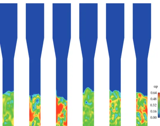
Fig. 16 shows instantaneous fields of volume fraction for

dif-ferent values of the restitution coefficient and boundary condition

Fig. 15. Radial profile of the time-averaged particle kinetic energy normalized by the square of fluidization velocity. Upper panels: effect of the wall boundary conditions (with the particle-particle restitution coefficient ec¼0.9), bottom panel: effect of particle-particle normal restitution coefficient, left panels: rough wall boundary conditions,

type. It is clear that for ec¼1 the distribution of solid in the reactor

is much more homogeneous than in case of eco1. The formation of bubbles is observed with both No–slip and Free–slip boundary conditions. This trend was also shown byFig. 13where the var-iance of the solid volume fraction was found to decrease with increasing particle-particle restitution coefficient.

Fig. 17 shows the probability density function of the solid

volume fraction in a test–cylinder located at the centre of the reactor. The peak of probability moves towards large volume fraction as the normal restitution coefficient decreases.

The presence of the mesoscale particle collective motion leads also to larger fluctuations of the vertical solid velocity as shown by

Fig. 14. In contrast, the particle kinetic energy decreases with

decreases in the normal restitution coefficient. This tendency is expected because according to the transport equation of the ran-dom particle kinetic energy, Eq.(A.21), the collisions lead to a sink term proportional to 1'e2

c.

The results are in accordance with those ofGoldschmidt et al.

(2001). Indeed Goldschmidt et al. (2001) observed that the

intensity of gas pressure fluctuations in the bed increases gradu-ally when the coefficient of restitution is decreasing. Such an increase of the pressure fluctuation intensity is typically related to increases in the variances of the solid volume fraction and the mean solid velocity, when the restitution coefficient is decreasing, as shown in the paper simulations. In addition,Goldschmidt et al.

(2001) showed, in accordance with these simulations presented

here, that a decrease in the restitution coefficient leads to a decrease in the random particle kinetic energy.

6.2. Effect of wall boundary conditions for the solid phase

The effect of the wall boundary conditions for the solid phase comes from two contributions: the boundary conditions on the mean solid velocity and that on the random particle kinetic energy.Figs. 3and4show that if only the wall-normal restitution coefficient is modified, which affects only the random particle kinetic energy boundary condition, no significant modification of the bed height is observed. In contrast, changing the wall boundary condition on the mean solid velocity leads to different vertical profiles of gas pressure and solid volume fraction.

The radial profile of the mean solid vertical velocity (Figs. 6and

7) shows that the smooth wall boundary conditions lead to a large downward solid velocity at the wall. In contrast, the downward velocity is reduced by using rough wall boundary conditions meaning that the effective friction of the particulate flow with the wall is increased.Figs. 6and7show no drastic effect of varying the

Fig. 16. Instantaneous solid volume fraction fields for different boundary conditions for the solid phase and different values of particle-particle restitution coefficient. From the left to the right; Free-slip and ec¼1.00, Free-slip and ec¼0.95, Free-slip and ec¼0.80, No-slip and ec¼1.00, No-slip and ec¼0.95, No-slip and ec¼0.80.

Fig. 17. Probability density function of the solid volume fraction in a cylinder defined such as '0:5rr=Rr0:5 and 0:5rz=Rr3:5 for different values of particle-particle restitution coefficient and wall boundary type.

wall-normal restitution coefficient from ew¼1.00 to ew¼0.86 on

the mean solid vertical velocity. As a matter of fact, ew is not

affecting directly the mean velocity boundary condition but might be effective through the modification of the random kinetic energy. However,Fig. 15shows that ewhas no effect on the radial

profile of random kinetic energy when using smooth boundary condition and will not affect the mean solid velocity either. As discussed inSection 5.3, the dependence of the random particle kinetic energy on the wall-normal restitution coefficient for the rough wall boundary conditions is more complex. Decreasing ew

should lead to a decrease of qp2and should decrease the friction of

the particulate flow with the wall. But for the typical values of the specularity coefficient used in the paper simulations (

ϕ

¼ 0:01 to 1), the dissipation of random particle kinetic energy due to wall-normal restitution coefficient looks negligible compared to the kinetic energy transfer from the mean particulate flow due wall roughness effect.

7. Conclusions

Numerical simulations of pressurized dense fluidized bed have been performed with an Euler-Euler approach. The effect of the particle-particle restitution coefficient and wall boundary condi-tions for the solid phase have been investigated. Two kinds of boundary conditions have been used: rough wall boundary con-ditions (Johnson and Jackson (1987)and No-slip) and smooth wall boundary conditions (Sakiz and Simonin (1999)and Free-slip).

The time-averaged Eulerian solid vertical velocity component has been compared with experimental measurements obtained by Positron Emission Particle Tracking. The time-averaged solid ver-tical velocity from the numerical simulations is in good agreement with the experimental data. It has been shown that the numerical predictions may be improved by using rough wall boundary con-ditions. The analysis of the time-averaged solid velocity fields showed that the Free-slip boundary condition leads to a macro-scopic toroidal (donut shape) circulation loop. In contrast, No-slip or Johnson and Jackson's boundary conditions, with a large value of the specularity coefficient ð

ϕ

Z0:1Þ, lead to two counter-rotating mixing toroidal loops.

A detailed analysis of the role of the boundary conditions on the Eulerian solid velocity and on the random particle kinetic energy has been performed. It has been shown that, in such a fluidized bed, the boundary conditions on the Eulerian solid velocity are of much more importance than those on the random particle kinetic energy. Finally the No–slip boundary condition for the mean particle velocity supplemented with zero flux boundary condition for the random particle kinetic energy are found to be good and effective approximations for solid wall boundary con-ditions representing particle-wall interaction with large roughness effects leading to predictions in satisfactory agreement with PEPT experimental data.

Nomenclature Subscripts

k _{k¼g: gas phase, k¼p: particulate phase} wall value at the wall

Latin symbols

Cd drag coefficient, [—–]

dp particle diameter, [m]

D_{p;ij particle strain rate tensor, ½rms}' 1₎

ec particle-particle normal restitution coefficient, [–]

ew wall-normal restitution coefficient, [–]

g0 radial distribution function, [–]

gi ith component of the gravitational acceleration, ½m=s2₎

Hbed mean height of the fluidized bed, [m]

Kp granular diffusivity, ½m2=s)

Kpcol collisional granular diffusivity, ½m2_=s)

Kpkin kinetic granular diffusivity, ½m2=s)

np particle number density ðnpmp¼

α

p

ρ

pÞ, ½m' 3)

ms solid mass in the reactor, [kg]

Pg gas pressure, [Pa]

qp2 random particle kinetic energy, ½m2=s2)

R internal radius of the fluidization column, [m] Rep particle Reynolds number, [–]

Uk;i ith component of the mean velocity of the phase k, [m/s]

Up;τ mean particle velocity tangent to the wall, [m/s]

Vf fluidization velocity, [m/s]

Vr gas-particle mean relative velocity, [m/s]

Greek symbols

α

p solid volume fraction, [–]

α

pmax maximum solid packing, [–]

Δ

characteristic grid width, [m]

Δ

n dimensionless characteristic grid width, [–]

μ

g dynamical gas viscosity, [kg/m/s]

μ

w wall-normal dynamic friction coefficient, [–]

ν

p kinetic viscosity of the phase k, ½m2=s)

ν

pcol collisional granular viscosity, ½m2=s)

ν

pkin kinetic granular viscosity, ½m2=s)

ϕ

specularity coefficient, [–]

ρ

g gas density, ½kg=m3)

ρ

p particle density, ½kg=m3)

Σ

k;ij kinetic stress tensor of the phase k, ½kg=m=s2)

τ

c collision time scale, [s]

τ

pSt particle response time based on Stokes law, [s]

τ

gpF particle response time, [s]

Acknowledgements

This work was granted access to the HPC resources of CALMIP under allocation P0111 (Calcul en Midi- Pyrénées). This work was performed using HPC resources from GENCI-CINES (Grant 2015-x20152b7423).

This work has been done in the frame of a long-term colla-boration with INEOS Technology Centre, Lavéra (FRANCE).

Appendix A. Mathematical model

This appendix gives the set of equations of the multi-fluid Eulerian model. In the following when subscript k¼g we refer to the gas and k¼p to the particulate phase.

The mass balance equation (without interphase mass transfer) is written ∂ ∂t

α

k

ρ

kþ ∂ ∂xj

α

k

ρ

k Uk;j¼ 0 ðA:1Þ

where

α

kis the volume fraction of the phase k,

ρ

kthe material

density and Uk;ithe ithcomponent of the k' phase mean velocity.

It must be noted that

α

p

ρ

prepresent npmpwhere npis the number

density of p-particle centers and mpthe mass of a single p-particle.

fraction of the dispersed phase. Hence, gas and particle volume fractions

α

gand

α

pshould satisfy

α

pþ

α

g¼ 1.

The mean momentum transport equation is written

α

k

ρ

k ∂ ∂t þUk;j ∂ ∂xj ' ( Uk;i¼ '

α

k ∂_Pg ∂xiþ

α

k

ρ

k g_iþIk;i' ∂

_Σ

_k;ij ∂xj ðA:2Þ

where Pgis the mean gas pressure, githe gravity acceleration and

Σ

k;ijthe effective stress tensor. In Eq.(A.2), Ik;i is the mean

gas-particle interphase momentum transfer without the mean gas pressure contribution. According to the large particle to gas den-sity ratio, only the drag force is acting on the particles. The mean gas-particle interphase momentum transfer term is written as: I_{p;i¼ '}

α

p

ρ

p

Vr;i

τ

F gp

and I_{g;i¼ 'Ip;i}: ðA:3Þ

The particle relaxation time scale is written 1

τ

F gp¼ 3 4

ρ

g

ρ

p 〈_{j v}rj 〉 dp Cd ðA:4Þ

where Cdis the drag coefficient. To take into account the effect of

large solid volume fractionGobin et al. (2003)proposed the fol-lowing correlation for the drag coefficient

Cd¼

minðCd;Erg; Cd;WYÞ if

α

p40:3

Cd;WY otherwise

(

ðA:5Þ where Cd;Ergis the drag coefficient proposed byErgun (1952):

C_{d;Erg¼ 200}

α

p Repþ

7

3 ðA:6Þ

and Cd;WY byWen and Yu (1965):

Cd;WY¼ 0:44

α

' 1:7 g if RepZ1000 24 Rep 1þ0:15Re 0:687 p 0 1

α

' 1:7 g otherwise 8 > < > : : ðA:7Þ

The particle Reynolds number is given by Rep¼

α

g

ρ

g〈j vrj 〉dp

μ

g

: ðA:8Þ

The mean fluid-particle relative velocity, Vr;i, is given in terms of

the mean gas and solid velocities: V_{r;i¼ Up;i'Uf ;i}. The solid stress tensor is written

Σ

p;ij¼

α

p

ρ

poup;i0 u0p;j4þ

Θ

_p;ij ðA:9Þ where u0

p;iis the fluctuating part of the instantaneous solid velocity

and

Θ

p;ij the collisional particle stress tensor. The solid stress

tensor is expressed as (Boëlle et al., 1995;Ferschneider and Mège, 2002;Balzer, 2000),

Σ

p;ij¼ Pp'

λ

pDp;mm

+ ,

δ

ij'2

μ

pD~p;ij ðA:10Þ

where the strain rate tensor is defined by ~ Dp;ij¼ Dp;ij' 1 3Dp;mm

δ

ij with Dp;ij¼ 1 2 ∂_Up;i ∂x_j þ ∂_Up;j ∂x_i ' ( : ðA:11Þ

The granular pressure, viscosities and model coefficients are given by Pp¼ 2 3

α

p

ρ

pq2p+1þ2

α

pg0ð1þecÞ, ðA:12Þ

λ

p¼ 4 3

α

2p

ρ

pdpg0ð1þecÞ ffiffiffiffiffiffiffiffiffi 2 3 q2 p

π

s ðA:13Þ

μ

p¼

α

p

ρ

p

ν

kinp þ

ν

colp 0 1 ðA:14Þ

ν

kin p ¼ 1 2

τ

Fgp 2 3q2pð1þ

α

pg0

ζ

Þ= 1þ

σ

₂

τ

F gp

τ

c " # ðA:15Þ

ν

col p ¼ 4 5

α

pg0ð1þecÞ

ν

kinp þdp ffiffiffiffiffiffiffiffiffi 2 3 q2 p

π

s 2 4 3 5 ðA:16Þ

ζ

¼2_5ð1þecÞð3ec'1Þ ðA:17Þ

σ

¼1_5ð1þecÞð3'ecÞ: ðA:18Þ

The collision time scale

τ

cis given by

1

τ

c¼ 4

π

g₀nqd2p ffiffiffiffiffiffiffiffiffiffiffi 2 3

π

q2p r ðA:19Þ where the radial distribution function, g0, is computed according

toLun and Savage (1986)as

g0ð

α

pÞ ¼ 1'

_α

α

p max

' (' 2:5αmax

ðA:20Þ where

α

max¼ 0:64 is the closest random packing.

The solid random kinetic energy transport equation is written:

α

p

ρ

p ∂q2 p ∂t þUp;j ∂q2 p ∂xj " # ¼ '_∂∂_x j

α

p

ρ

p Kkin p þKcolp 0 1∂q2_p ∂xj " # '

Σ

p;ij ∂_Up;i ∂x_j '

α

_τ

p_F

ρ

p gp 2q2 p '1₃1'e 2 c

τ

c 2 3q2p: ðA:21Þ

In Eq.(A.21), the first term on the right–hand–side represents the transport of the random particle kinetic energy due to the particle agitation and the collisional effects. That term is written by introducing the diffusivity coefficients:

Kkin_p ¼2₃q2_p5 9

τ

Fgp 1þ

α

pg0

ζ

c = >= 1þ5₉

τ

F gp

ξ

c

τ

c ' ( ðA:22Þ Kcol_p ¼

α

pg0ð1þecÞ 6 5Kkinp þ 4 3dp ffiffiffiffiffiffiffiffiffi 2 3 q2 p

π

s 2 4 3 5 ðA:23Þ

ζ

c¼ 3

5ð1þecÞ2ð2ec'1Þ ðA:24Þ

ξ

c¼ð1þecÞð49'33e₁₀₀ cÞ: ðA:25Þ

The second term on the right-hand-side of Eq.(A.21)represents the production of particle agitation by the gradients of the mean solid velocity. The third term is the interaction with the gas. Finally the fourth term is the particle agitation dissipation by inelastic collisions.

Appendix B. Numerical implementation of wall boundary conditions

This appendix is dedicated to the detailed description of the numerical implementation of the boundary conditions for the solid phase mean velocity and random kinetic energy.

According to part3.2, the flat frictional wall boundary condi-tions can be written in the following generic forms:

ν

p ∂Up;τ ∂n # $ wall ¼ A q2p h i wall ðB:1Þ

Kp ∂_Up;τ ∂n # $ wall ¼ B q2p h i wall 0 13=2 ðB:2Þ where A and B are two given parameters of the modelling approach.

For computing the solid wall shear stress and random kinetic energy wall flux effects in the transport equation resolution method, the numerical approach implemented in NEPTUNE_CFD uses a first order gradient approximation between the computed variables at the wall distance Ycand fictitious imposed variables at

the wall (as shown onFig. 18B), so the above equations are written in the frame of the numerical code approach as,

ν

pAYc=2BUp;τ Yc f g' U+ p;τ,imp Yc ¼ A q 2 p h i wall KpAYc=2B q2 pf g' qYc 2p h iimp Yc ¼ B q 2 p h i wall 0 13=2

where

ν

pAYc=2B and KpAYc=2B represent the effective particle

viscosity and diffusivity used in the frame of the numerical code approach for the flux computation in the diffusion step resolution method and they are chosen equal to the computed value at Yc.

Then the fictitious imposed values of the solid mean velocity and random kinetic energy at the wall are written,

Up;τ + ,imp ¼ Up;τf g'Yc A Yc

ν

pf gYc q2_p h i wall q2_p h iimp ¼ q2pf g'Yc B Yc Kpf gYc q2_p h i wall 0 13=2

Finally, the fictitious variables, used as Dirichlet wall boundary conditions, are directly written in terms of the computed variables at Ycby assuming a low variation of the random particle kinetic

energy between Ycand dp=2, so that:

Up;τ + ,imp ¼ Up;τf g'Yc A Yc

ν

pf gYc q2_pf gYc ðB:3Þ q2_p h iimp ¼ q2pf g'Yc B Yc Kpf gYc q2_pf gYc 0 13=2 ðB:4Þ According to partSection 3.3, the Johnson and Jackson's rough wall boundary conditions can be written in the following generic forms:

ν

p ∂Up;τ ∂_n # $ wall¼ A g0 + , wall Up;τ + , wall q 2 p h i wall 0 11=2 ðB:5Þ Kp ∂q2_p ∂n ! wall ¼ 'A g+ 0,wall Up;τ + , wall = >2 q2_p h i wall 0 11=2 þB g+ 0,wall q2p h i wall 0 13=2 ðB:6Þ

where A and B are two given parameters of the modelling approach.

According to the numerical approach implemented in NEPTU-NE_CFD, the solid wall shear stress and random kinetic energy wall flux are written in the numerical code approach as,

ν

pAYc=2BUp;τ Yc f g' U+ p;τ,imp Yc ¼ A g0 + , wall Up;τ + , wall q 2 p h i wall 0 11=2 KpAYc=2B q2_pf g' qYc 2p h iimp Yc ¼ 'A g0 + , wall Up;τ + , wall = >2 q2_p h i wall 0 11=2 þB g+ 0,wall q2p h i wall 0 13=2

As previously, the effective particle viscosity and diffusivity used in the frame of the numerical code approach for the flux computa-tion in the diffusion step resolucomputa-tion method are chosen equal to the computed value at Ycand the fictitious imposed values of the

mean particle velocity and random kinetic energy are written, Up;τ + ,imp ¼ Up;τf gYc '

_ν

A Yc pf gYc g0 + , wall Up;τ + , wall q 2 p h i wall 0 11=2 q2_p h iimp ¼ q2pf gYc þ

_ν

A Yc pf gYc g0 + , wall Up;τ + , wall = >2 q2_p h i wall 0 11=2 '_KB Yc pf gYc q2_p h i wall 0 13=2

The above Dirichlet wall boundary conditions are written in practice assuming a low variation of the random particle kinetic energy between Ycand dp=2: q2p

h i

wall¼ q 2

pf g and by computingYc

the pair distribution function using the solid volume fraction computed at Yc: g+ 0,wall¼ g0f g. But, in contrast, specific numer-Yc

ical sensitivity analysis, carried out with the numerical code, have shown that the computation of Up;τ

+ ,

wall, the ”true” mean

trans-lation particle velocity at the distance dp=2 from the wall, needs

special care, especially for large roughness effects corresponding to large value of An ¼ AYcg0 ffiffiffiffiffi q2 p q

=

ν

p(when An is in the order of or

larger than 1).

So, an approximation of U+ p;τ,_wallis derived from the solid wall

shear stress written in terms of the mean particle translation velocity defined at Ycand dp=2 using the values predicted at Ycfor

the solid viscosity, pair distribution function and random particle kinetic energy:

ν

pf gYc Up;τf g' UYc + p;τ,imp Yc'dp=2 ¼ A g0 + , wall Up;τ + , wall q 2 p h i wall 0 11=2

then, the mean tangential velocity of the particles in contact with the wall is written,

Up;τ + , wall¼ Up;τf g 1þYc A Y= c'dp=2>

ν

pf gYc g0f g qYc 2pf gYc 0 11=2 ' (' 1 ðB:7Þ Finally, using the above equation for U+ p;τ,_wall, the fictitious

vari-ables, used as Dirichlet wall boundary conditions, may be written in terms of computed variables at Yconly by using the following

equations, Up;τ + ,imp ¼ Up;τf gYc '

_ν

A Yc pf gYc g0f g UYc+ p;τ,_wall q2pf gYc 0 11=2 ðB:8Þ q2_p h iimp ¼ q2pf gYc