Mining Frequent Subgraphs in Multigraphs

HAL Id: lirmm-01761235

https://hal-lirmm.ccsd.cnrs.fr/lirmm-01761235

Submitted on 8 Apr 2018

HAL is a multi-disciplinary open access archive for the deposit and dissemination of sci-entific research documents, whether they are pub-lished or not. The documents may come from teaching and research institutions in France or

L’archive ouverte pluridisciplinaire HAL, est destinée au dépôt et à la diffusion de documents scientifiques de niveau recherche, publiés ou non, émanant des établissements d’enseignement et de recherche français ou étrangers, des laboratoires

Mining Frequent Subgraphs in Multigraphs

Vijay Ingalalli, Dino Ienco, Pascal Poncelet

To cite this version:

Vijay Ingalalli, Dino Ienco, Pascal Poncelet. Mining Frequent Subgraphs in Multigraphs. Information Sciences, Elsevier, 2018, 451-452, pp.50-66. �10.1016/j.ins.2018.04.001�. �lirmm-01761235�

Mining Frequent Subgraphs in Multigraphs

a_{LIRMM - University of Montpellier, France} b_{UMR TETIS, Irstea, Montpellier, France}

Abstract

For more than a decade, extracting frequent patterns from single large graphs has been one of the research focuses. However, in this era of data eruption, rich and complex data is being generated at an unprecedented rate. This complex data can be represented as a multigraph structure - a generic and rich graph representation. In this paper, we propose a novel frequent subgraph mining approach MuGraM that can be applied to multigraphs. MuGraM is a generic frequent subgraph mining algorithm that discovers frequent multigraph patterns. MuGraM efficiently performs the task of subgraph matching, which is crucial for support measure, and further leverages several optimization techniques for swift discovery of frequent subgraphs. Our experiments reveal two things: MuGraM discovers multigraph patterns, where other existing approaches are unable to do so; MuGraM, when applied to simple graphs, outperforms the state of the art approaches by at least one order of magnitude. Keywords: Graph Mining, Multigraphs, Frequent Subgraphs.

1. Introduction

Real world data can be easily modelled as a graph where entities are represented as nodes, and interactions between entities are represented as edges. When only one edge type is allowed between a pair of nodes, we refer to this graph structure as single edge graph; when more than one edge type is allowed between a pair of nodes, we refer to it as multigraph. Multigraph structure enables us to represent multiple relations between a pair of nodes [2, 3]. Many real world datasets can be modelled as a network where a set of nodes are intercon-nected by multiple relations. Various domains are abound with multigraphs: social networks spanning over the same set of people, but with di↵erent life aspects (e.g., social relationships such as Facebook, Twitter, LinkedIn, etc.); protein-protein interaction multigraphs, where the protein pairs have direct interactions/physical associations or they are co-localised [1]; gene multigraphs, where genes are connected by di↵erent pathway interactions that belong to di↵erent pathways; Resource Description Framework (RDF) knowledge graphs, where a subject/object node pair is connected by di↵erent predicates [17].

Email addresses: [email protected] (Vijay Ingalalli), [email protected] (Dino Ienco), [email protected](Pascal Poncelet)

1,2,3

2,4

2,5 2 2,3 1,2,4 3

1 : lunch 2 : facebook 3: coauthor 4 : leisure 5 : work

(a) A sample data multigraph

3 2 1,2 2,4 2,3 2 P₁ P₂

(b) A set of frequent multigraph patterns

Figure 1: (a) A data multigraph with unlabeled nodes; (b) a set of multigraph patterns with frequency = 2

Since multigraphs allow more than one relation between a pair of nodes, we can repre-sent real world data more succinctly, which in turn helps in mining patterns that cannot be discovered in the otherwise simple graphs. For example, a recent work in the field of bioinformatics [16] creates multigraphs by merging heterogeneous genomic and phenotype data, in order to identify the disease genes. Many such applications can be catalysed in order to mine interesting and useful patterns.

One of the most important tasks in graph data management is frequent subgraph mining (FSM) [11, 13, 22, 14, 6] where the problem is to discover patterns that occur frequently in a graph database. Although plenty of approaches exist to mine frequent patterns in single edge graph, to the best of our knowledge, no approach exists to mine frequent patterns in multigraphs.

Considering FSM in single edge graph data, the existing approaches can be categorized into two main families: (i) FSM for transactional graph setting, where the graph database consists of a set of relatively small sized graphs called transactions, and (ii) FSM for single large graph setting, where the graph database consists of a single large graph.

In transactional graph databases, a subgraph is frequent if it appears in at least transac-tions, where is a user defined frequency threshold value. Several works have been proposed to address FSM in transactional graph databases [11, 13, 22]. However, since the task of FSM in single large graph setting is more challenging than the transactional one, several ap-proaches [14, 6] have been proposed by considering various frequency (or support) evaluation measures [20, 4].

This work is motivated by the fact that the existing FSM approaches cannot be applied to multigraph data. That is, when the graph data contains multiple relations between a pair of entities, the existing FSM approaches cannot discover frequent patterns that contain a subset of multiedges. Thus, whenever multiple relations (multiedges) exist between a pair of nodes, in order to use the existing FSM approaches, one has to map the multiple relations (multiedges) to a unique value (distinct edge label) and then perform FSM, which however, does not yield desirable results, thereby making the existing approaches rather incomplete. To the best of our knowledge, no existing work can discover frequent subgraphs in single large multigraphs. It is to be noted that one of the recent works called GraMi [6] claims

to handle multi-labeled graphs (which we refer to as multigraphs). However, neither they provide any details about managing multigraphs in their paper, nor their latest code is capable of handling multigraph data.

Let us consider a typical scenario of performing FSM on a multigraph as depicted in Figure 1. The data multigraph in Figure 1a is an extract of the real world AUCS dataset [12] that has five di↵erent relations (edge types) namely, lunch, facebook, coauthor, leisure, and work which are defined among a set of university employees (nodes). If we perform FSM on this dataset by setting a frequency threshold = 2, the existing FSM approaches output no patterns, since they treat a set of relations between a pair of nodes as a unique identifier, rather than treating it as a set of multiple relations. And thus, they are unable to discover those frequent patterns that are spanned from a subset of the relations, as depicted in Figure 1b.

The objective of the proposed work is to fill the gap in the field of FSM by proposing an approach to extract frequent patterns from multigraph data by considering patterns that can span over a subset of the multigraph relations. Thus, we propose MuGraM (Frequent MultiGraph Miner ) - an algorithm that enumerates all frequent subgraph patterns in a single large multigraph. The major contributions of this work are:

• a set of efficient pruning rules to swiftly traverse the search space for multigraph pattern extraction;

• an efficient method to quickly evaluate the pattern support;

• a quantitative and qualitative evaluation of MuGraM on real world graph data. The experimental evaluation reveals that MuGraM is not only an approach that can handle multigraph data efficiently but it also outperforms the state-of-the-art approaches in extracting frequent subgraphs in single edge graph data.

The rest of the paper is organized as follows. In Section 2, we discuss the related works. In Section 3, we introduce some basic definitions and formalize the problem. In Section 4, we discuss the proposed multigraph mining algorithm MuGraM along with several opti-mization strategies. Detailed experimental evaluations are conducted in Section 5, followed by the conclusion in Section 6.

2. Related work

Several existing works address the problem of FSM for both transactional graph databases and single graph databases. For the transactional graph database setting, the work of Inokuchi et al. [11] has shaped the foundation for many later works. This work proposed an approach called AGM to efficiently mine the association rules among the frequently appear-ing substructures in a given graph data set, by treatappear-ing a transaction as an adjacency matrix. Among the later works, few are notable: FSG by Kuramochi and Karypis [13] that models the problem of finding frequent graphs as a subgraph discovery problem; gSpan by Yan and Han [22], that discovers frequent substructures without candidate generation. Other related

works include significant pattern mining Leap [21], and maximal frequent subgraph mining Margin [19].

Works on single large graph databases can be traced back to Subdue [9], that used minimum description length principle to discover substructures that compress the database, which was further improved later [8]. The work of Kuramochi and Karypis [14] mentions two approaches namely, vSiGraM, and hSiGraM, based on depth first search and breadth first search respectively. The underlying principle followed was to grow the frequent patterns only from the smallest sized frequent patterns. The frequency of a subgraph was computed by addressing the problem of subgraph isomorphism. Since the problem of subgraph isomor-phism is NP-complete [15], they proposed efficient ways to compute support by storing the exact location of each frequent subgraph, which is faster but at the cost of more memory. In this work, they also introduced the notion of canonical representation to check if two patterns are isomorphic or not, in order to avoid any redundant pattern generation.

One of the most recent FSM approaches for single large graphs is GraMi [6], wherein they model the problem of frequency evaluation as a constraint satisfaction problem (CSP), that requires a costly subgraph isomorphic matching operation; however, this avoided the enumeration of all the embeddings, which was deemed expensive in Kuramochi et al. [14]. GraMi also proposed a heuristic search with novel optimizations that significantly improved the performance by pruning the search space. In addition, GraMi also proposed an ap-proximate version of the algorithm. The latest work DistGraph, proposed by Talukder and Zaki [18], is a distributed approach to address FSM in single large graph settings.

In this paper, we propose an approach called MuGraM that finds exact patterns in a single large multigraph. In this direction, we take inspiration from GraMi by avoiding the exhaustive enumeration of the embeddings of a pattern, which was followed in vSi-GraM and hSivSi-GraM [14]. In vSi-GraMi, support is addressed by solving a CSP, whereas in MuGraM, we employ backtracking approach that is commonly used in the field of graph database to address subgraph isomorphism [15]. In order to mine multigraph patterns, Mu-GraM leverages the backtracking approach which explores the topology of the input graph by incorporating vertex ordering techniques for pattern subgraphs (Section 4.6.1). Although GraMi incorporates several optimization techniques related to CSP, MuGraM proposes optimization strategies that are curated for backtracking approach in order to handle multi-graphs. Further, employing backtracking approach with depth first search (DFS) traversal allows MuGraM to be more flexible in terms of traversing the search space (Theorem 2); this reduces the time taken to reach the support threshold thereby expediting the overall support computation. To the best of our knowledge, no work exists to perform FSM on multigraphs. Although MuGraM is curated to address multigraphs, our experiments (Sec-tion 5) confirm that MuGraM is also computa(Sec-tionally efficient for FSM on standard single edge graphs.

3. Preliminaries and problem definition

In this paper we address the problem of mining single large multigraphs with undirected edges and unlabelled vertices, which will be referred as multigraphs. A multigraph G is

defined as a tuple (V, E, LE, T ), where V is a set of vertices, T is a set of edge types,

E _{✓ V ⇥ V is a set of undirected edges, and L}E : V ⇥ V ! 2T is a labelling function that

assigns a subset of edge types to each edge E it belongs to. The labeling function LE maps

the edge E to a multiedge, and thus G is a multigraph.

Since one of the challenges in FSM process is to check the existence of a subgraph in a data multigraph, we formalize the subgraph isomorphism problem for multigraphs as follows. Definition 1. Subgraph isomorphism for multigraphs. Given a multigraph pattern P = (Vp_{, E}p_{, L}p

E, Tp) and a multigraph G = (V, E, LE, T ), the subgraph isomorphism from P to

G is a function : Vp _{! V such that,}

8(um, un)2 Ep, 9 ( (um), (un))2 E and LpE(um, un)✓ LE( (um), (un)).

A pattern P is subgraph isomorphic to _{G if there exists at least one subgraph Q in G} that is isomorphic to P ; i.e., Q is an isomorphic embedding of P in G. Further, if P is subgraph isomorphic to _{G, then there exists a set of embeddings of P in the multigraph G.} The problem of enumerating all the isomorphic embeddings of P in_{G is a classic problem of} subgraph matching [15]. In Section 4, we discuss the problem in the context of multigraphs. From now on, a sub-multigraph pattern P will be simply referred to as a pattern.

The embeddings of a pattern P in a given multigraph _{G play a crucial role for the} task of graph mining. To evaluate the frequency of a subgraph, one needs to check if the number of isomorphic embeddings of a pattern in a given graph is at least , where is the user defined frequency threshold. However, since the isomorphic embeddings in a single graph can potentially overlap, there might be a violation of the anti-monotonicity property that is crucial in pruning the search space during mining [4]. The property of anti-monotonicity guarantees that if any pattern P of size s is found to be infrequent, then all possible extensions of pattern P will be infrequent. This property is essential for an FSM algorithm, since the general idea of FSM is to discover the smallest frequent patterns initially and then grow the frequent patterns until no more frequent patterns are discovered. Many works have been proposed that introduce various ways of measuring frequency, referred to as support measures, that are anti-monotonic [7, 14, 4]. Among all these support measures, minimum node image (MNI) support measure [4] is one of the most computation-ally efficient support measure. As proposed in [6], in this paper we use the MNI support measure to extract frequent patterns.

1,2,3

2,4

2,5 2 2,3

1,2,4

3

2 : facebook 3: coauthor 4 : leisure

Definition 2. Minimum Node Image (MNI) support. Given a pattern P and a multigraph G, let E = {E1, E2, . . . , En} be the set of n isomorphic embeddings of P in G, and i be a

function i : Vp ! V for each embedding Ei. Then the minimum node image (MNI) support

for a pattern P is defined as (P ) = minv2Vp|{ _i(v) : i = 1, . . . , n}|.

For an intuitive understanding, consider the example in Figure 1. To measure the MNI support for the pattern P1, we enumerate the embeddings of the pattern P1, as depicted in

Figure 2. As we observe, every vertex of pattern P1 has a unique image in the data graph

and 2 distinct embeddings imply that for each pattern vertex, the node image is 2. That is, the image of a vertex is the number of distinct vertices belonging to a set of matched embeddings. Thus, for pattern P1, the MNI support is (P1) = 2, since the minimum of

the image size of all the nodes is 2.

With this background, we now introduce the problem of FSM in multigraphs. Mining multigraphs to discover frequent sub-multigraphs is the problem of frequent sub-multigraph pattern mining, formally defined as follows.

Problem 1. Frequent sub-multigraph pattern mining. Given a multigraphG, and a support threshold , discover the entire set of patterns _{P in G, such that (P)} .

In the following section, we propose an efficient graph mining algorithm MuGraM, that seamlessly extracts frequent multigraph patterns from a single large multigraph.

4. MuGraM: An algorithm for mining multigraphs

In order to address the problem of FSM for single large multigraph data, we propose MuGraM - a frequent multigraph mining algorithm. Our proposed approach follows a framework similar to that of existing mining approaches, as introduced in [14, 6]. A generic framework (as depicted in Figure 3) of mining single large graphs involves the following steps: (i) enumerate the frequent edges (frequent patterns of size s = 1), (ii) extend each frequent pattern by successively adding the frequent edges recursively, (iii) avoid repeated pattern generation, and (iv) compute the support of the newly generated patterns to decide if the pattern is frequent or not. Before getting into the details, we introduce some concepts to understand the operations of mining multigraphs.

4.1. Multi-edge representation and pattern enumeration

Since in a multigraph the basic pattern is a multiedge, one might compute the MNI support of each multiedge E in a given multigraph G, to discover the frequent multiedges. However, this set of frequent multiedges is rather incomplete. To perform exact mining, it is necessary to enumerate the subsets of the multiedges, and then compute their support to decided if they are frequent or not; we refer to such frequent subsets of the multiedges as a set of frequent seeds P1_.

Definition 3. Frequent seeds. A set of frequent seeds P1 _{is a union of each frequent subset}

f of all the distinct multiedges E. Given a multigraph G with n distinct multiedges, a set of frequent seeds is represented as, P1 _=[n

Input graph G, support value δ Enumerate the frequent multiedges

Perform subgraph extension

Is the subgraph frequent?

Entire search space traversed?

Terminate Collect frequent subgraphs Yes No Yes No

Figure 3: The framework of MuGraM for FSM in multigraphs

For example, consider a multigraph G with two distinct multiedges E1 = {e1, e2, e3}

and E2 = {e2, e3, e4}, that occur exactly once. If one is interested in finding patterns with

support threshold 2, then without enumerating the subsets of multiedges, we would have no frequent patterns, which is incorrect. By enumerating the subsets of multiedges, we discover three frequent patterns, each of size s = 1, which have multiedges _{e2}, {e3}

and _{e2, e3} respectively. Thus, the set of frequent seeds for G is represented as P1 =

{{e2}, {e3}, {e2, e3}}.

4.2. Overview of MuGraM

The proposed approach MuGraM is summarised in Algorithm 1. MuGraM takes a multigraph G and the support threshold measure as input, and outputs a set of patterns P that satisfy the minimum frequency threshold w.r.t. MNI support measure. MuGraM maintains a set of frequent patterns P, a set of non-frequent patterns NP, a set of canonical

representation C of each frequent pattern, a stack S that contains the nodes of the DFS tree of search space and an iterator ne, which are initialized in line 3. As a first step, we enumerate the set of frequent seeds P1_{, that contains the frequent patterns of size s = 1}

(line 4). To enumerate the frequent seeds, we firstly collect the existing multiedges in G along with the subsets of multiedges. Then we compute the number of occurrences of each multiedge and quickly verify with respect to the MNI measure, whether they appear at least

times. Thus, the set of frequent seeds is represented as P1 _={f

1, . . . , fn}.

Since an efficient way of exploring the search space for single large graphs is to traverse in a DFS manner, as endorsed in [14], we follow the DFS traversal of the search space. MuGraM discovers frequent patterns by recursively extending the frequent patterns P1

of size s = 1, by traversing the search space in a DFS manner (lines 6-10). Further, we propose to order the set of frequent seeds P1 _{with the increasing order of their frequency}

of occurrence. Thus, we define the partial order (P1_{, ), where is a relation on the}

Algorithm 1: MuGraM

1 Input: A multigraph G, support threshold 2 Output: All frequent patterns P in G

3 Initialize: P =;, S = ;, N_P =;, C = ;, ne = 0 4 Enumerate: All frequent seeds (multiedges) P1

5 Ordering: Maintain a partial order (P1, ), where is a relation on frequency

value

6 for every f 2 P1 do

7 EP = {f_e 2 P1 :8f 2 P1, f_e ⌫ f}

8 S .push(f ) /* Stack of f for DFS mining */

9 P= P [ FindFreqPatterns(EP, ne, , S , C , N_P, G)

10 ne = ne + 1

11 return P

the frequent patterns, the ordering of the frequent edges in the increasing order of their frequency value is beneficial to quickly decide whether the new patterns are frequent or not. For each frequent seed f , we collect a set of extendible seeds _{EP (line 7), where f}e is a

frequent seed that is used to extend f . The set of extendible seeds is used to extend a given frequent seed f in a recursive manner, and the criterion of selection of EP is described in Section 4.3. The procedure FindFreqPatterns (line 9) discovers the frequent patterns in a DFS manner, as depicted in Algorithm 2. A stack data structure S manages the nodes of the DFS tree traversal, which is initialized in line 8. Thus for each frequent multiedge f 2 P1_,

we invoke the procedure FindFreqPatterns (Algorithm 2) to find the subsequent frequent patterns of size s > 1 (line 9). All the discovered frequent patterns are collected in P. Before getting into the details of FindFreqPatterns procedure, we discuss about the search space spanned by MuGraM, which will in turn help in understanding the FindFreqPatterns procedure.

4.3. Search space spanned by DFS traversal

The search space of MuGraM in the beginning is spanned by a set of frequent seeds P1 = _{f1, . . . , fn}, where fi is a frequent seed (multiedge) or a frequent pattern of size

s = 1. In order to discover frequent patterns of size s > 1, we extend each frequent seed fi

with the set of frequent seeds P1_{. For example, given a set of frequent seeds P}1 _={f 1, f2},

in order to discover all the frequent patterns, one needs to explore the entire search space (generated by pattern extension) as shown in Figure 4a. Each node in the search space tree (as seen in Figure 4a) is a group of patterns of size s; e.g., the node in the search space tree f1-f2-f1 contains all the patterns of size s = 3 that can be generated by three edges

{f1, f2, f1}. Further, each node in the search space tree for size s > 1 represents a set of

child patterns of size s + 1 generated by extending its parent of size s. The search space grows from level s to s + 1 only if the patterns at the sth_{level are frequent. This exploration}

s = 1 s = 2 s = 3 f₂-f₂ f₁-f₁-f₁ f₁-f₁-f₂ f₁-f₂-f₁ f₁-f₂-f₂ f₂-f₁-f₁ f₂-f₁-f₂ f₂-f₂-f₁ f₂-f₂-f₂ f₂-f₁ f₁-f₂ f₁-f₁ f₁ f₂

(a) Original search space

f₂,f₂,f₂ f₂,f₂ f₂ f₁ f₁,f₂ f₁,f₁ f₁,f₂,f₂ f₁,f₂,f₁ f₁,f₁,f₂ f₁,f₁,f₁

(b) Compact search space

Figure 4: Search space for a set of frequent seeds P1₌

{f1, f2}

not-frequent, then any pattern that is an extension of P cannot be frequent. For example, the node f1-f2-f1 is generated by extending the pattern f1-f2, only if at least one pattern in

f1-f2 is frequent.

In simple terms, each frequent seed f 2 P1 _{is extended with the entire set of frequent}

seeds P1_{, where repeated extension are allowed; thus f}

1-f1 is a valid extension. However,

we propose that it is possible to reduce the search space traversal by making an interesting observation.

Theorem 1. Given a partially ordered set (P1_{, ), where is a relation on the set of}

frequent seeds P1_{, it is sufficient to extend a frequent seed f 2 P}1 _{with a set of seeds}

{fe 2 P1 : fe ⌫ f}.

Proof. Since the extension of frequent seeds generates pattern children of size s = 2, it would be sufficient to prove that at level s = 2, all possible patterns would be generated by the respective parents. And due to the antimonotonicity property [4] of the support measure, all possible frequent patterns would be discovered for s > 2. Now, given a multigraph G without any vertex labels and a set of n frequent seeds P1_{, ordered by a relation ,}

pattern extension generates a set of patterns of size s = 2, P2 _=[k

i=1{(fi efj) : fi, fj 2

P1, j = 1, . . . , k_{}, where} e is an edge extension operation so that all possible structures

are enumerated. For level s = 2, we observe that any two patterns, P1 = (fi efj) and

P2 = (fj efi) with i 6= j are pairwise isomorphic, and hence redundant. Thus, given a

relation , it would be sufficient to retain a pattern P = (fi efj) w.r.t. the order fi fj.

⌅

As a consequence of Theorem 1, we do not need to extend each frequent seed with all possible frequent seeds P1_{; this reduces the traversal of search space, and thus we are}

able to avoid many redundant mining operations. As depicted in Algorithm 1, line 7, each frequent seed f is extended only by a set of extendible frequent seeds _{EP. Intuitively, if} we observe Figure 4a, two patterns (colored in red) f1-f2 and f2-f1 are isomorphic to each

pattern f2-f1 can be safely discarded; further the search space extending from f2-f1 can be

discarded due to the antimonotonic property of the support measure, resulting in a much compact search space as depicted in Figure 4b.

4.4. Discovering frequent patterns

Frequent patterns are discovered in a recursive manner by following DFS traversal of search space, as depicted in Algorithm 2. Since the stack structure S stores the frequent patterns for the entire search space, we perform DFS exploration until the stack S is emptied. When the stack S becomes empty (line 3), we would have visited all possible patterns that are the extension of f 2 P1_{. This is repeated until all the elements have been}

extended, as observed in Algorithm 1, line 6.

Algorithm 2: FindFreqPatterns(_{EP, ne, , S , C , N}P, G) 1 if ne >|EP| then

2 return /* All edges extended */

3 while S is not empty do

4 P := S .top() /* Fetch the pattern to be extended */

5 P_e :=EP.ne /* The multiedge used for extension */

6 P_N := ExtendPattern(P , P_e, C , N_P) /* New patterns */

7 P_F := ComputeSupport(P_N, G) /* New frequent patterns */

8 if P_F 6= ; then

9 S .push(P_F) /* Stack grows with new FSGs */

10 P = P [ P_F

11 else

12 ne := ne + 1

13 FindFreqPatterns(EP, ne, , S , N_P, G)

14 S .pop() /* Stack shrinks in size */

15 Reset: ne

As we traverse the search space in a DFS manner (lines 3-15), we keep on extending the initial frequent seed f 2 P1_{. A pattern P to be extended is fetched (note that the stack}

size is not reduced) from the top of the stack S (line 4) and the corresponding multiedge Pe which is used for extending P (line 5) is chosen from the set of extendible edges EP.

We recall that a set of extendible edges EP contains a set of frequent patterns P1 _{of size}

s = 1. When a pattern P of size s is extended, a set of new patterns _PN of size s + 1 are generated. The ExtendPattern procedure performs this extension as shown in line 6. For this set of new patterns PN, the ComputeSupport (line 7) procedure computes

the support value and checks if there are any frequent patterns, which results in a set of frequent patterns PF ={P 2 PN : (P ) }; thus PF ✓ PN. For pattern extension, the

new frequent patterns inPF are added to the stack S , and further added to the repository

P is extended with the next multiedge by incrementing the pointer ne to choose the next multiedge _{EP.ne (line 12), and the FindFreqPatterns procedure is called recursively.} Once all the extendible edges Pe 2 EP have been used for extension, i.e., when ne > |EP|

(lines 1 - 2), the recursive call is terminated and the stack is reduced (line 14). The entire recursive procedure is repeated until the stack S is empty, thereby traversing the entire search space that spans from the initial frequent seed f _{2 P.}

4.5. Pattern extension

In Algorithm 3, we extend a pattern P with an extendable multiedge Pe, resulting in a

set of new patterns PN. A pattern P of size s can be extended to generate several patterns

of size s + 1 by attaching a multiedge Pe. However, depending on the structure of the

pattern P , we can attach Pe in two ways: (i) by introducing an additional vertex, and (ii)

by not introducing any additional vertex. For example, in Figure 5a, we can only extend the pattern P by introducing a node, whereas in Figure 5b we need to extend the pattern P by introducing a new node as well as without introducing an extra node (the new nodes used for extension are colored in green, while the dotted lines indicate all possible edge extensions). In Algorithm 3, the extension is done for every vertex of the pattern (lines 3 - 4), where the addition of an edge is done through P.add(Pe) operation.

Algorithm 3: ExtendPattern(P , Pe, C , NP) 1 Initialize: P := ;

2 V_a = ComputeAutoGroup(P ) /* Generate new patterns that are distinct

3 for every {v 2 V_a} and {[v_i, v_j]2 Vp : i6= j ^ i, j  |Vp|} do

4 Pnew = P.add(Pe) /* Node and edge extension */

5 Generate: C .P_new := CanRep(P_new)

6 if C .P_new is contained in C then

7 continue; /* Skip to next pattern */

8 if HasInfrequentChild(P_new, N_P) then

9 continue; /* Skip to next pattern */

10 InheritInvalid(P_new, P)

11 C := C [ C .P_new

12 P := P [ {Pnew}

13 return C , P

4.5.1. Optimization techniques during pattern extension

We now propose few optimization techniques that are employed during the pattern ex-tension procedure ExtendPattern.

Canonical verification: One of the challenges that is often faced in FSM approaches is the repeated generation of patterns. When we are traversing the search space by extending the frequent patterns, it is likely to happen that the same pattern was already generated.

f₁ f₄ f₂ f₃ f₁ f₂ f₃ f₄ f₄

(a) Extension only with an extra node f₃ f 1 f2 f₁ f₂ f₁ f₂ f₃ f₃ f₃

(b) Extension with and without an extra node f₁ f 4 f₂ f₂ f 1 f f2 2 f₄ f 4 u₁ u₂ u 3 u 4 u₄ u₁ u₂ u₄ u₃ (c) Extension considering automorphic groups

Figure 5: Various possible extensions of a pattern and automorphic grouping

Such repeated generations can be avoided by checking whether the new pattern is isomorphic to the already generated patterns. One of the efficient ways to perform this task is to compute the canonical representation for each pattern and store it in a repository called canonical repository. Whenever a new pattern is generated, we check whether it matches against the contents of canonical repository; if there is a match against a canonical representation in the repository, then the new pattern was already generated; else, the repository is updated with the canonical representation of the new pattern. This approach is proposed in [14], which we extend for multigraphs. For the ease of reading, we reproduce the definition of a canonical representation.

Definition 4 (Canonical representation). Canonical representation of a pattern P is an isomorphism-invariant labelling of the vertices of P . Thus if a pattern P is isomorphic to P0, then both P and P0 have the same canonical representation.

Whenever a new pattern is generated by an edge extension, we generate the canoni-cal representation of Pnew (line 5) and check if the pattern was already generated before

(lines 7-8). Thus, if the newly generated pattern is isomorphic to any of the already gener-ated patterns, we do not consider it for extension, since the new pattern has already been generated before; else, we update the corresponding canonical repository C (line 11), and continue to generate the next new pattern (lines 7)

Automorphic extension: While extending a pattern P with an extra node by an extendible edge Pe, instead of choosing each vertex v 2 Vp, it is sufficient to choose a set of

vertices for extension that belong to distinct automorphic groups of Vp _{[14]. This in turn}

reduces the overhead caused by computing the canonical representation for the extended new patterns Pnew, that is deemed redundant. For example, in Figure 5c, we are interested

in extending a pattern P that has a multiset of multiedges _{f1, f2, f2} with an extendible

frequent seed f4, using an extra node. The set of automorphic groups for the given pattern P

can be computed as{{u1, u3}, {u2}}. Since u1and u3belong to the same automorphic group,

it is sufficient to consider any of them; thus we can either use_{u1, u2} or {u3, u2} as a set of

vertices for extending with Pe. Thus, Vaconsists of a set of vertices belonging to the distinct

automorphic group as shown in Algorithm 3, line 2. The procedure ExtendPattern returns a set of new patterns _{P, and the corresponding canonical representations C .}

Detecting infrequent patterns: When we traverse the search space in a DFS manner, we collect a set of infrequent patterns NP (to be discussed later in Algorithm 4). Whenever

a new pattern is generated, we check if the new pattern Pnew is a supergraph of any of

the infrequent patterns in NP, as depicted in lines 8-9. This avoids the expensive support

computation, since we are able to quickly detect that the new pattern is infrequent due to the anti-monotonicty property of the support measure.

Once it is confirmed that the newly generated pattern Pnew is not infrequent and was

never generated before, we update the set of new patterns_{P (line 12). Once the pattern P} has been extended in all possible ways, the procedure ExtendPattern returns the set of newly generated patternsP, and the updated canonical repository C .

4.6. Support computation for multigraphs

Computing the support of a pattern is one of the most crucial aspects of any graph mining algorithm, as one has to address the NP-complete problem of subgraph isomorphism. This becomes even harder when we are dealing with multigraphs, as we have to tackle the more generic version of the problem of sub-multigraph isomorphism [10].

Thus, in this section, we propose an efficient algorithm for support computation by ad-dressing three crucial questions: (i) how to efficiently enumerate the isomorphic embeddings of a multigraph pattern in order to compute the support of a pattern, (ii) assuming that a pattern is frequent, how fast can we find a set of embeddings of a pattern so that MNI support threshold is reached quickly, and (iii) how quickly can we decide if a pattern is not frequent. In the following sections, we will address these three issues in the mentioned order. 4.6.1. Sub-multigraph matching

In this section we address the first question of enumerating the isomorphic embeddings for a given multigraph pattern by formulating the problem of sub-multigraph matching which is formally defined as follows.

Problem 2. Given a pattern P , and a multigraph G, discover the entire set of embeddings E = {e1, . . . , el} such that every ei 2 E is a sub-multigraph of G and ei is isomorphic to P .

The multigraph matching problem involves a much basic problem of solving multigraph isomorphism as described in Definition 1. To address the problem of sub-multigraph matching, we take inspiration from the work of Ingalalli et al. [10], where a subgraph matching approach called SuMGra, especially tailored for multigraphs, is pro-posed. The subgraph matching procedure involves two important steps in order to enumerate the isomorphic embeddings:

• Ordering of the pattern vertices. A fixed ordering of the pattern vertices is maintained since an efficient ordering is essential for faster discovery of embeddings. Given a pattern P with a vertex set Vp _={u

1, . . . , un}, a linearly ordered set is defined as the

• A backtracking approach to enumerate embeddings. A set of isomorphic embeddings are discovered by following the already defined vertex order, where the search space is spanned in a DFS manner following a backtracking approach.

For example, considering a pattern P with a vertex set Vp _={u

2, u3, u1}, and a linearly

ordered set (Vp_{, <), u}

2 is the first vertex to be matched and u1 is the last vertex to be

matched. The backtracking approach outputs an embedding only when all the pattern vertices are matched, and the matching is performed in the mentioned order. With a fixed vertex ordering, the principle of backtracking approach enables us to explore the entire search space, which eventually leads to the enumeration of the entire set of embeddings.

However, in this work, since we focus on checking if a pattern P appears in G at least times w.r.t. the MNI measure, we do not need to exhaustively compute all the embeddings. Instead, we only need to carefully span the search space to discover a set of embeddings that are sufficient enough to reach the MNI support threshold. Thus, we propose an efficient way of enumerating the embeddings to quickly reach the MNI support threshold.

4.6.2. Efficient support evaluation

In this section, we discuss about enumerating a set of embeddings of a multigraph pat-tern whose objective is to quickly reach the MNI support threshold. To achieve efficient computation of MNI support value, we modify the backtracking approach of sub-multigraph matching proposed in [10].

Consider a pattern P for which we want to evaluate the support value to decide if it is frequent; in order to reach the support threshold value of , we must enumerate at least isomorphic embeddings of the pattern P . In the best case scenario, number of embeddings would be enough to reach the MNI threshold value of ; however, to achieve this, the isomorphic embeddings should be non-overlapping (two embeddings e1 and e2 are

overlapping, if they share at least one vertex) in such a way that the image of each pattern vertex is at least . Recalling the definition of MNI support (Definition 2), an image of a pattern vertex is the number of distinct vertices belonging to a set of matched embeddings. Thus, the challenge for any subgraph matching approach is to enumerate such embeddings in an efficient manner.

The necessity for efficient enumeration of embeddings to reach MNI support threshold can be understood by revisiting the functioning of the backtracking procedure. Let us recall that the existing backtracking approach of sub-multigraph matching problem SuMGra [10], discovers a set of embeddings by traversing the subgraph search space in a DFS manner. And this backtracking approach follows a fixed ordering (Vp_{, <) on the set of pattern vertices}

Vp _={u

1, . . . , un}, where u1 is matched first and un is matched at the end. Subsequently a

set of vertices Vm _{of an isomorphic embedding m 2 M are enumerated in that order, and}

since we follow the backtracking approach, the distinct matched vertices for un are

replen-ished faster than the distinct matches for u1; thus if we allow the embeddings discovered

through the backtracking approach, the image of vertex ungrows much faster than the image

of vertex u1, leading to an asymmetrical distribution of image values of pattern vertices.

(Algorithm 4) that enumerates the isomorphic embeddings by allowing the pattern vertices to achieve the maximum possible image with minimum number of embeddings.

The intuition of the ComputeSupport procedure is to enumerate the isomorphic em-beddings to achieve uniform distribution of image values for the set of pattern vertices Vp_.

This can be achieved by considering a set of n vertex orderings = _{ 1, . . . , n} for a

pattern P with n vertices, rather than one fixed ordering. Further, if we allow each vertex ordering i to have a distinct initial vertex ui, each vertex ui will occupy the first position

of the order, which forces the vertex matches to be distributed more uniformly across all the pattern vertices.

However, from the previous section we recall that one fixed ordering will allow the back-tracking procedure to explore the entire search space. If we allow a set of _{| |= n vertex} orderings, we would span the search space n times, which is an overhead. Thus to avoid this overhead, we propose to modify the backtracking search. Let us assume that an initial pattern vertex u1 has l potential vertex matches; in order to discover the embeddings, in a

normal backtracking approach, the search begins from each of these l initial vertex matches until all possible embeddings are discovered. Thus, in a normal backtracking search that starts from one of the matches, say lk, the entire solution space is spanned as the

backtrack-ing search discovers the complete set of embeddbacktrack-ings. However, in the modified approach, the backtracking search of a particular path is terminated as soon as an embedding is discovered. Instead of allowing the backtracking search to traverse the entire solution space with lk as

the initial match, we proceed further to traverse the search space using the next potential match lk+1. This process is repeated until all the potential matches have been considered

thereby avoiding the last pattern vertex un to receive an unfairly large number of distinct

matches.

In Theorem 2 it is shown that if the backtracking procedure is terminated for each search path, and the backtracking process is allowed for n vertex orderings, the entire search space would be spanned.

Theorem 2. Considering a pattern with n vertices and the corresponding set of vertex per-mutations that has n distinct orderings, where each ordered vertex set begins with a distinct pattern vertex ui, it is sufficient to terminate the backtracking procedure once an embedding

is discovered in a particular DFS traverse; i.e., by restarting the backtracking procedure for each vertex permutation i 2 , we will enumerate all the embeddings of a pattern.

Proof. For a given linearly ordered vertex set (Vp_{, <) of a pattern P with n vertices,}

the backtracking procedure traverses the entire search space by recursively performing DFS search for the pattern vertex matches [10]. To achieve this, a single vertex set ordering, say i is sufficient to span the entire search space, since each pattern vertex is recursively

allowed to find the corresponding isomorphic match. Now, if we allow the backtracking to be performed for a permutation of vertex set ordering of size n, where each vertex order permutation i has ui as its initial vertex in the ordering, we can then terminate the

backtracking process for that DFS search path once an embedding is found. The rest of the embeddings that could exist in this DFS path will be discovered by following another vertex

As a consequence of Theorem 2, we can reach the support threshold in a more symmetric manner, which in turn helps us to quickly decide if a pattern P is frequent.

Algorithm 4: ComputeSupport(N PC, NP, , G)

1 Initialize: FP_C =; /* A set of frequent patterns */

2 for each P 2 N P_C do

3 := ComputePerm(Vp) /* Permutation ordering of vertices in P */

4 Cand := FindInitCandidates(Vp, P , G)

5 Initialize: E :={ei =; : i = 1 ! |Vp|} /* Embeddings of P */

6 Set: P.f requent = F alse;

7 for each permutation _k 2 do

8 Fetch: im = InvalidMatches(P , uk)

9 Cand( _k) :={Cand( _k)\ im \ e_i : i = k}

10 if |Cand( _k)|< then

11 break; /* The pattern in infrequent */

12 if CollectEmbeddings(P , _k, Cand( _k), G, E ) then

13 P.f requent = T rue;

14 FP_C =FP_C[ P /* Pattern P is frequent */

15 break; /* Skip to next pattern */

16 if P.f requent = F alse then

17 N_P = N_P [ P /* Pattern P is not frequent */

18 return FP_C

Referring to Algorithm 4, let us consider a pattern P with |Vp_{|= n vertices; for pattern}

P , we compute n distinct vertex order permutations ={ 1, . . . , n}, where a permutation k represents a vertex ordering with ui as its initial vertex (line 3). Thus, by considering

every permutation k2 , we would have considered each vertex ui 2 Vp as the initial vertex

for the backtracking procedure. Before applying the backtracking procedure, the potential matches for each vertex ui 2 Vp are enumerated using the FindInitCandidates procedure

(line 4) as proposed in [10]; we call these matches as the initial candidate set Cand. The discovered embeddings are stored in E where each set ei 2 E , initialized with an empty set,

stores the matched vertices of a pattern vertex ui. Thus, the size of |ei| denotes the image

of the pattern vertex ui.

We now discuss the backtracking approach to discover isomorphic embeddings by fol-lowing a set of vertex orderings (lines 7-15). For each pattern vertex permutation i, the

CollectEmbeddings procedure (Algorithm 5) is invoked (line 12) in order to collect the embeddings of pattern P . If the image of all pattern vertices is at least then the MNI sup-port has been reached and hence we collect the frequent pattern P to fetch the subsequent pattern by returning to the previous procedure (line 14-15).

In Algorithm 5, we propose the CollectEmbeddings procedure that enumerates the embeddings required to quickly reach support threshold. For every matched initial vertex

v 2 Cand( k), we recursively find an isomorphic match (lines 7-8). Whenever a match is

found, i.e., when _{|Emb|= |V}p_{|, the embedding is collected and the image of each pattern}

vertex is evaluated; and when the image of all the pattern vertices have reached the threshold , we terminate the procedure as the pattern P is frequent (lines 9-12). One important factor where the proposed CollectEmbeddings procedure di↵ers from a backtracking procedure to discover isomorphic embeddings is that every time an embedding is found, instead of backtracking to enumerate the next embedding, we terminate the backtracking process and restart the matching procedure for the next vertex v_{2 Cand(} k); this ensures

symmetric distribution of image values of the pattern vertices.

However, even after RecursiveMatching procedure, no embedding is discovered, i.e., |Emb|< |Vp_{|, then for the initial pattern vertex u}

k, the initial vertex match v 2 Cand( k)

is not a valid match since there exists no embedding in _{G with the initial match v. Thus,} the vertex v can be considered as an invalid match for the pattern vertex P.uk, and hence

the AssignInvalidMatches procedure assigns vertex match v as an invalid match for the pattern vertex P.uk (line 14). Once all the initial matches have been considered for

com-puting the embeddings using the RecursiveMatching procedure, the algorithm returns back to ComputeSupport to fetch the next vertex order permutation.

Algorithm 5: CollectEmbeddings(P , k, Cand( k), G, E ) 1 PotentialMatchesSize: P M :=|Cand( _k)|+|b_k|

2 for each v 2 Cand( _k) do

3 if P M < then

4 P.f requent = f alse; /* Pattern P is infrequent */

5 return false;

6 Emb = {v} /* A match for initial vertex u₁ */

7 for each pattern vertex u2 { _k\ u₁} do

8 Emb = Emb [ RecursiveMatching(u, P , G)

9 if |Emb|= |Vp| then

10 E = E [ Emb /* Collect the new embedding */

11 if {|e_i| : i = 1! |Vp|} then

12 return true; /* Pattern P is frequent */

13 else

14 AssignInvalidMatches(P.u_k, v)

15 Decrement P M = P M 1

16 return false;

4.6.3. Optimization techniques during support computation

In this section we address the third question that was raised in the beginning which is about quickly deciding if a pattern is not frequent. Since the search space of mining

frequent patterns grows exponentially, especially in the case of multigraphs, the proportion of infrequent patterns collected in comparison to the discovered frequent patterns also increases. Thus, we spend more time on infrequent patterns to attest their infrequency than to decide if a pattern is frequent. While in the previous section, the ComputeSupport procedure promoted the idea of quickly deciding if a pattern is frequent, it also helps to some extent in deciding if a pattern is infrequent. We now discuss about the optimization strategies which have been proposed as part of Algorithms 4 and 5, which will help us to predict that a pattern is infrequent even without spanning the entire search space.

Managing infrequent patterns: Recalling Algorithm 4, whenever we find a pattern P to be infrequent, we add it to the repository of infrequent patterns NP (line 16-17). This

repository is maintained as a hierarchical collection of infrequent pattern structures w.r.t. their sizes. Whenever a new pattern is generated during the pattern extension procedure ExtendPattern (Algorithm 3), we fetch all the infrequent patterns that are smaller than the new pattern, and check if any of them is subgraph isomorphic to the new pattern; if so, then the new generated pattern cannot be frequent due to anti-monotonicity principle.

Managing invalid matches of pattern vertices: As we just discussed on leveraging the information of infrequent patterns for early prediction of further infrequent patterns, we now focus on how can we leverage crucial information from frequent patterns and use them to decide the infrequency of subsequent patterns. When we observe the procedure CollectEmbeddings (Algorithm 5), we initially have a set of potential candidate matches Cand. k(u1) for the initial vertex u1 of a pattern P . The initial vertex u1 is fetched from a

permutation of vertex order k. The RecursiveMatching procedure in line 8, manages to

find the matches to the rest of the vertices k\u1 of pattern P , using backtracking approach,

which yields an isomorphic solution of the pattern P . However, if RecursiveMatching procedure cannot find an isomorphic matching, then the potential match v 2 Cand. k(u1)

for the initial vertex u1 is indeed an invalid match, since no embedding exists in the entire

search space. Thus, we can safely assign v as an invalid match for the initial vertex u1 of

pattern P . Note that we can assign the invalid matches only for the initial vertex u1 since

the search space exploration for an embedding begins from that vertex.

Further, if the pattern at level s + 1 is an extension of a pattern at level s, we can exploit the anti-monotonicity property in order to push the invalid matches of a pattern at level s to the pattern of level s + 1. And since we traverse the search space in a DFS manner, we cumulatively collect the invalid matches as we go down the search space. Thus, whenever a new pattern is generated during the pattern extension procedure FindFreq-Patterns, as depicted in Algorithm 2, we pass on the invalid matches as depicted by the InheritInvalid procedure (line 14). Thus when a new pattern Pnew is evaluated for its

support measure by Algorithm 4, it already contains a set of invalid matches for all the vertices Vp_{. This information is exploited to refine the candidate matches in Algorithm 4,}

line 9. Thus the candidate matches for the initial vertex u1 2 k are pruned by the

opera-tion: Cand( k) :={Cand. k(u1)\ InvalidMatches( k(u1))}, thereby reducing the number

of candidate matches. This significantly reduces the computational overhead on the back-tracking procedure RecursiveMatching in Algorithm 5 (line 8). Further, the reduction in the size of the potential matches Cand helps to decide if a pattern can reach the support

threshold; i.e., for a given permutation ordering k, if the size of the potential matches is

less than the support threshold Cand. k< , then there is no need to compute the support,

since the pattern cannot have embeddings. This optimization is exploited in Algorithm 4, lines 10-11, and in Algorithm 5, lines 3-5.

4.7. Complexity analysis and convergence of MuGraM

Temporal complexity. One of the steps that is computationally intensive in the proposed MuGraM is support evaluation, as outlined in ComputeSupport (Algorithm 4). As al-ready discussed in Section 3, support computation involves the problem of subgraph isomor-phism matching, which is NP-complete [15]. If we consider a multigraph G with V vertices and a subgraph pattern with u vertices, the computation of subgraph isomorphism takes O(Vu_{) time. Further, the task of generating all the subgraphs ofG has a time complexity of}

the order ofO(2V2

). The task of canonical verification to check for the repeated generation of a subgraph (isomorphic testing) has a complexity of _{O(V ! ) [14]. Thus the upper bound} on the time complexity of mining a graph is O(Vu_{· 2}V2

· V ! ), which is exponential in the graph size. Although the theoretical upper bound is exponential on graph size, in practice, the heuristics involved in each of the computationally intensive procedures, drastically re-duce the time taken by MuGraM. Even though the canonical representation for isomorphic testing takes O(V ! ), the algorithm [14] that incorporates several vertex invariants, reduces the time complexity. Further, in MuGraM, the procedure ComputeSupport to compute support (Algorithm 4) involves several optimizations (Section 4.6.3) that reduce the time complexity. For the procedure of pattern extension ExtendPattern (Algorithm 3), sev-eral optimization techniques (Section 4.5.1) that have been proposed contribute in reducing the complexity.

Spatial complexity. Apart from being computationally expensive, the task of FSM also leads to substantial memory consumption. For a given graph _{G, as the number of} fre-quent subgraphs grow, the spatial complexity increases. This growth is exponential in space complexity, especially when the intermediate results are stored for efficient computation as in [22, 14]. However, MuGraM manages memory efficiently; the overall memory consuming procedure in MuGraM is FindFreqPatterns (Algorithm 2). Since MuGraM follows DFS strategy, the FindFreqPatterns procedure needs to store information only along the depth of the search space, as already seen in Figure 4. Thus, the stack data structure S that contains all the frequent subgraphs, and the hashmap containing the canonical repre-sentations C together consumeO(n·|Ef

p|) space, where |Epf| is the size of a frequent pattern,

and n is the number of discovered frequent patterns. Further, if m non-frequent patterns are encountered while checking the support value, then the hashmap NP has a space complexity

of O(m · |Enf

p |), where |Epnf| is the size of a non-frequent pattern. Thus, the overall space

complexity during the process of FSM is_{O(mn · |E}f

p||Epnf|). It is important to note that the

space consumed by the hashmap data structure NP is significantly lower when compared

to the theoretical upper bound; the space is reduced due to several optimization strategies as proposed in Section 4.6.3.

Convergence. The convergence of MuGraM needs to be demonstrated under two di↵er-ent circumstances. Firstly, we need to show that the pattern space does not grow indefinitely.

This fact is partly supported by Theorem 1, where we prove that a subset of frequent seeds is sufficient enough to extend a frequent seed, so that the entire search space is spanned to discover the frequent patterns. Further, the principle of anti-monotonicity [4] guarantees to inhibit the growth of subgraph search space; thus, if a subgraph pattern is found to be infre-quent, then the entire subsequent search space is pruned. Secondly, it suffices to show that the backtracking approach terminates. Recalling Section 4.6, the backtracking approach operates in a DFS manner in the search space spanned by pattern embeddings. Referring to Theorem 2, it can be concluded that the backtracking approach which was employed in Algorithm 4 terminates irrespective of the pattern being frequent or non-frequent.

5. Experimental analyses

In this section we evaluate the performance of MuGraM by carrying out both quantita-tive and qualitaquantita-tive analysis. For quantitaquantita-tive evaluation, we compare the time performance of MuGraM with one of the recent state-of-the-art FSM approach - GraMi; for this eval-uation, we use single edge graphs since no approach exists to perform FSM on multigraphs. Further, the qualitative analysis is performed on few real-world datasets to demonstrate the nature of patterns extracted by the proposed multigraph mining approach MuGraM.

All the experiments were conducted on a server with 64-bit Intel 6 processors @ 2.60GHz, and 250GB RAM, running on a Linux OS - Ubuntu 14.04 LTS. MuGraM is implemented in C++.

5.1. Quantitative evaluation: Time performance evaluation

In order to evaluate the time performance of MuGraM, we use a variety of real world datasets with varying size and density. Table 1 lists the datasets and their properties that we use to evaluate the time performance of MuGraM and compare it with the recent state-of-the-art approach GraMi.

Dataset # Vertices # Edges # Edge types Density

DBLP-Mappedgraph 83 901 141 471 910 Medium

Citeseer 3 312 4 732 27 Medium

Microsoft 100 000 1 080 298 240 Dense

Amazon 334 863 925 872 1 Medium

Table 1: Properties of the graph datasets indicating the number of vertices, edges, edge types and graph density

DBLP-Mappedgraph is built from the original DBLP-Multigraph dataset by mapping the multiedges in the original dataset to a set of distinct values. The original dataset DBLP-Multigraph1 _{is built by following the procedure adopted in [2], where the vertices correspond}

to di↵erent authors and each edge type represents one of the top 50 Computer Science

conferences. Two authors are connected by an edge type if they co-authored at least one paper together in that conference. Thus, in the original dataset, a pair of authors can be co-authors for more than one conference and hence can share more than one edge type. For example, the original dataset may contain a multiedge with three edge types {e1, e3, e8}.

Since the existing approaches can discover patterns with only one edge type, we use the mapped dataset in order to compare MuGraM with GraMi.

CiteSeer dataset is a graph created with ‘publications’ as nodes and ‘citations’ between a pair of publications as edges. Each node has a single label representing the field of Computer Science. The distinct edge types are the similarity measures among the corresponding pair of publications, which vary in the range 0 to 100, where a smaller value implies stronger similarity. Microsoft dataset contains co-authorship information, and is represented as an undirected graph where unlabelled nodes represent the authors and edges represent collabo-ration between two authors; the various edge types correspond to the number of co-authored papers. Both CiteSeer2 _{and Microsoft}2_{] datasets are provided by the authors of GraMi [6].}

Amazon3 _{dataset was created by crawling Amazon website. It is based on the ‘Customers}

Who Bought This Item Also Bought’ feature of the Amazon website. If a product p is frequently co-purchased with product p0_{, then graph contains an undirected edge from p}

to p0_{. This dataset contains only unlabelled edges and has been chosen to evaluate the}

performance of MuGraM when dealing with simple graphs.

All the experiments have been conducted for increasing values of support threshold that are specific to a dataset. Further, in order to discover the frequent patterns, a maximum execution time of 1 day was allotted for each support threshold value; the time taken to discover patterns is reported in seconds (on a logarithmic scale) only after the corresponding algorithms terminate within the allotted time.

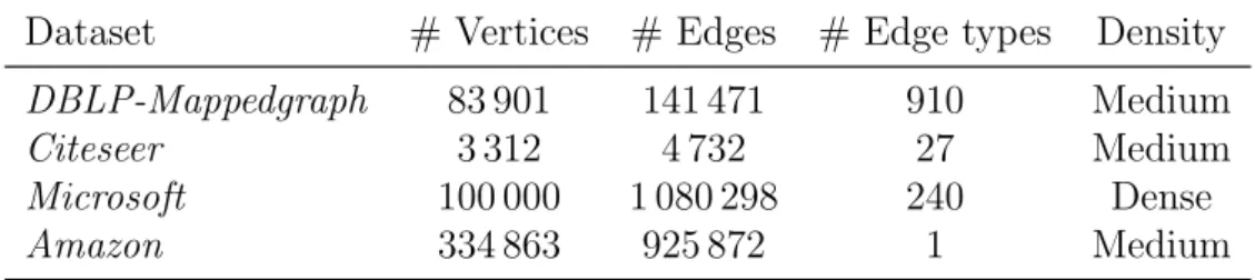
The time performances for all the four datasets are depicted in Figure 6. For Amazon dataset (Figure 6a), where we vary the support value from 300k to 296k (300,000 to 296,000), we observe that MuGraM outperforms GraMi by 2-3 orders of magnitude although Ama-zon is a simple graph with only one edge type (not a multigraph). Further, for support values from 297k, GraMi fails to terminate within the allocated maximum execution time of 1 day, while MuGraM is able to successfully terminate. For DBLP-Mappedgraph dataset (Figure 6b), we observe that MuGraM outperforms GraMi with almost 1-2 orders of magnitude, where the support values are varied from 3.5k to 2.7k. For Citeseer dataset (Figure 6c), we observe that the time performance of MuGraM is 2-3 orders of magnitude better than GraMi for higher support values, although for relatively lower support value of 100, MuGraM outperforms GraMi by _{⇠1 order of magnitude. For Microsoft dataset} (Figure 6d), both MuGraM and GraMi are able to terminate within the allotted time of 1 day for the entire support range of 41k to 36k. For higher support values, MuGraM is ⇠1 order of magnitude better than GraMi, while the performance gap shrinks slightly for the lower support values.

We perform an additional quantitative analysis in order to test the potentiality of the

2_{http://github.com/ehab-abdelhamid/GraMi/tree/master/Datasets} 3_{http://snap.stanford.edu/data/com-Amazon.html}

(a) Amazon (b) DBLP-Mappedgraph

(c) Citeseer (d) Microsoft

Figure 6: Time performance of (a) Amazon (b) DBLP-Mappedgraph (c) Citeseer and (d) Microsoft datasets

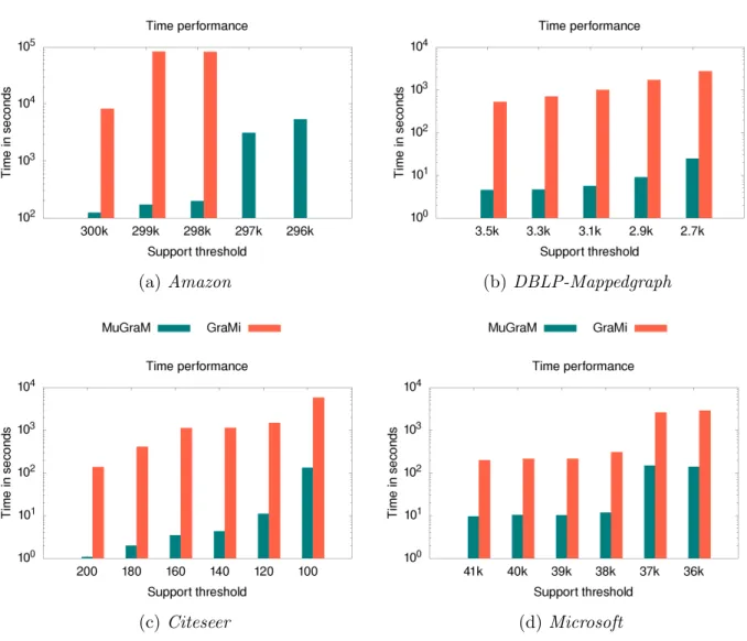
proposed framework. We perform this test by comparing the performance of MuGraM on the original DBLP-Multigraph and the transformed DBLP-Mappedgraph. Figure 7 depicts the behaviour of multigraph and mapped-graph performances; in Figure 7a, we compare the number of patterns discovered for the two versions of the same DBLP dataset, and we observe that we are able to discover patterns for DBLP-Multigraph that cannot be discovered using DBLP-Mappedgraph. Thus we are loosing patterns by transforming the multigraphs to mapped-graphs. Further, we also evaluate the time performance of MuGraM when employed to mine multigraphs. In Figure 7b, we observe that DBLP-Multigraph needs some amount of additional time to discover multigraph patterns which did not exist in the case of DBLP-Mappedgraph. However, it is important to note that this additional time grows only linearly for multigraphs when compared to the corresponding mapped-graphs, although multigraphs pose a tougher challenge in terms of search space than the

(a) No. of patterns outputted (b) Time performance

Figure 7: Comparison of time performance and number of outputted patterns for DBLP dataset

corresponding mapped-graphs.

5.2. Performance Evaluation of MuGraM Optimizations

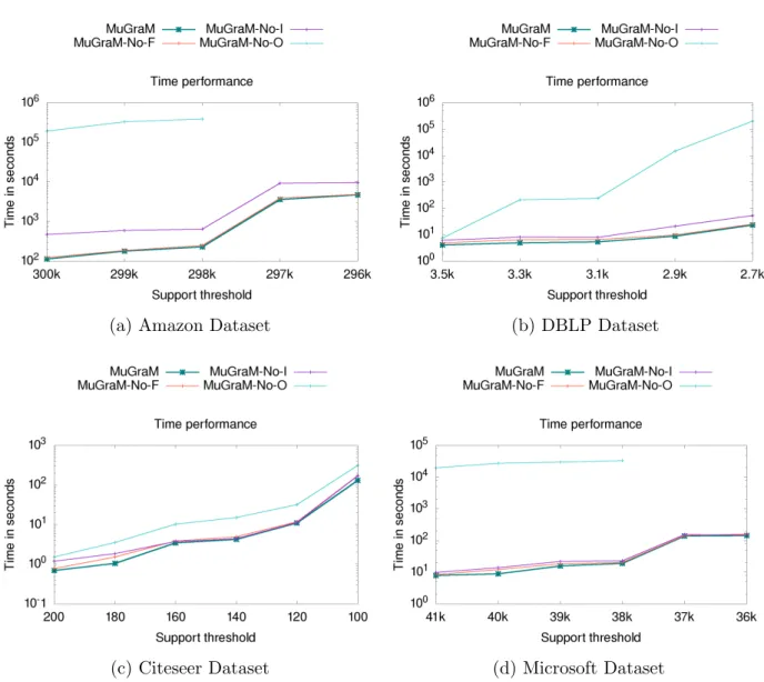
In this section, we evaluate the impact of the optimizations that have been proposed during the di↵erent stages of MuGraM. In order to e↵ectively analyse the impact of opti-mizations on the performance of MuGraM, we introduce the following three settings where for each setting, one of the optimizations is disabled.

MuGraM-No-F. In this setting, we do not employ the optimization that maintains a repository of infrequent patterns NP, which is used to check if a newly generated pattern

is frequent or not. Recall that this optimization allows us to avoid the expensive operation of support computation.

MuGraM-No-I. For this setting, we do not collect invalid matches for the vertices of each newly generated patterns. Recall that the invalid matches collected for each pattern were propagated down the search space, thereby improving the performance even when we move deep down to mine bigger patterns. Thus, by not using this optimization, we are considering all possible matches as valid matches which would increase the search space.

MuGraM-No-O. For this setting, we do not generate di↵erent permutations of vertex or-dering, and thus, the DFS traversal is not discontinued once an embedding is found. By turning o↵ this optimization, more number of embeddings have to be enumerated in order to reach the support threshold thereby a↵ecting the time performance.

As observed in Figure 8, the performance of MuGraM deteriorates for the MuGraM-No-F setting; the performance degrades for DBLP (Figure 8b), Citeseer (Figure 8c) and Microsoft (Figure 8d) datasets for higher support values, where as for Amazon (Figure 8a)

dataset, the performance is much like MuGraM. For MuGraM-No-I setting, the per-formance deteriorates for Amazon (Figure 8a) dataset; for DBLP (Figure 8b), Citeseer (Figure 8c) and Microsoft (Figure 8d) datasets the performance is relatively better, but still poorer than MuGraM. Considering the setting MuGraM-No-O, we observe that for Amazon (Figure 8a) and Microsoft (Figure 8d) datasets, the performance of MuGraM drastically deteriorates and for lower support values, support threshold takes more than the permissible time of 24 hours; for Citeseer (Figure 8c) and DBLP (Figure 8b) datasets, the support threshold is reached within the permissible time, although the performance is significantly poor.

To summarize, we observe that all the optimizations introduced in the proposed mining approach improve the time performance of MuGraM, where the significant improvement is contributed by: i) the permutation of the vertex ordering, and ii) the propagation of invalid matches during the search space traversal. The first optimization clearly improves the performance of MuGraM by some order of magnitudes on three datasets (Amazon, DBLP and Microsoft). Further, the optimization related to the repository of infrequent patterns helps to improve the performance of MuGraM although its contribution is less crucial compared to the other two optimisation strategies.

5.3. Qualitative analysis

We conduct qualitative analysis for the following two datasets, and employ MuGraM to discover the frequent patterns. Since the discovered patterns are frequent patterns, it is important to note that they reveal the most common behaviour of a set of users/entities (nodes).

ATN: The ATN [5] dataset is an Air Transportation Network data that describes airline companies operating in Europe during the year 2011. The dataset is represented as a multi-layered graph, where the nodes and edges represent airport locations and routes, respectively, and each layer corresponds to a di↵erent airline company. In the original dataset, there are 417 nodes, 3 588 edges and 37 layers. We map this data into a multigraph dataset, with 417 nodes and 2 953 multiedges.

For ATN dataset, we extract multigraph patterns by setting MNI support threshold = 15, and report few interesting patterns, as depicted in Figure 9a. Pattern P1 depicts

a frequent behaviour of three airports a, b and c interconnected by Scandinavian airlines, where a and c are additionally connected by Norwegian airlines. Since these three airports are strongly connected by forming a clique, we can deduce that such pattern could be revealing a common behaviour where the three airports could belong to bigger cities (with more passenger traffic), and hence more likely to be capital cities. And since the carriers are Scandinavian and Norwegian, the three cities probably belong to Scandinavian countries.

Pattern P2 depicts a frequent situation in which four airports (a,b,c and d) are involved.

Airport a appears to be a major airport hub from where many links exist (from a to b, c and d). With this pattern being frequent, we can deduce that a major airport (a) often o↵ers connectivity to airports with relatively lesser air traffic (b, c, d). In this particular pattern, since all the airlines belong to Germany, a could be the busiest airport in Germany.

(a) Amazon Dataset (b) DBLP Dataset

(c) Citeseer Dataset (d) Microsoft Dataset

Figure 8: Evaluation of MuGraM optimizations for (a) Amazon (b) DBLP (c) Citeseer (d) Microsoft datasets

MRM: The MRM [12] dataset is provided by MIT Media Lab. It represents human interactions using mobile phones. The dataset is a multi-layered graph where the nodes represent users and the edges represent the way they interact with each other. The dataset has four di↵erent layers that represent di↵erent ways of communication namely, phone calls, friendship claims, bluetooth proximity scans, and text message exchanges. We map the original dataset to a multigraph with 94 nodes and 3 079 multiedges.

For MRM dataset, we extract multigraph patterns by setting MNI support threshold = 30, and report few interesting patterns as depicted in Figure 9b. In Figure 9b, pattern P1 depicts a frequent behaviour involving six users (nodes), where one user is pivotal (here

a) to the interaction pattern. Although the user a has a direct interaction with b and c through phone calls and text messages, a is in proximity with d and e, who together form