Design of emergent and submerged rock-ramp fish passes

(1)

O

pen

A

rchive

T

OULOUSE

A

rchive

O

uverte (

OATAO

)

OATAO is an open access repository that collects the work of Toulouse researchers and

makes it freely available over the web where possible.

This is an author-deposited version published in :

http://oatao.univ-toulouse.fr/

Eprints ID : 18368

To link to this article : DOI:

10.1051/kmae/2016032

URL :

http://dx.doi.org/10.1051/kmae/2016032

To cite this version :

Cassan, Ludovic and Laurens, Pascale Design

of emergent and submerged rock-ramp fish passes. (2016)

Knowledge and Management of Aquatic Ecosystems, vol. 417 (n°

45). pp. 1-10. ISSN 1961-9502

Any correspondence concerning this service should be sent to the repository

administrator:

staff-oatao@listes-diff.inp-toulouse.fr

(2)

R

ESEARCH

P

APER

Design of emergent and submerged rock-ramp ﬁsh passes

Ludovic Cassan

*

and Pascale Laurens

Institut de Mecanique des Fluides, allee du Prof. Camille Soula, 31400 Toulouse, France

Abstract – An analytical model is developed to calculate the stage-discharge relationship for emergent and submerged rock-ramp fish passes. A previous model has been modified and simplified to be adapted to a larger range of block arrangement. For submerged flows, a two-layer model developed for aquatic canopies is used. A turbulent length scale is proposed to close the turbulence model thanks to a large quantity of data for fully rough flows from the literature and experiments. This length scale depends only on the characteristic lengths of arrangements of obstacles. Then the coefficients of the logarithmic law above the canopy can also be deduced from the model. As a consequence, the total discharge through the fish pass is computed by integrating the vertical velocity profiles. A good fit is found between the model and commonly observed values for fish pass or a vegetated canopy. The discharge of the fish pass is then accurately estimated for a large range of hydraulic conditions, which could be useful for estimating fish passability through the structure.

Keywords: rock-ramp / ﬁshpass / design / hydraulic resistance / turbulence

Résumé – Dimensionnement de passes à poissons constituées de rampes à macrorugosités émergées et immergées. Un modèle analytique a été développé pour déterminer la relation de dimensionnement de passes à poissons constituées de rampes à macrorugosités émergées et immergées. Un modèle proposé précédemment a été modifié et simplifié afin de couvrir un éventail plus large de configurations géométriques. Pour des macrorugosités immergées, un modèle à deux couches pour des écoulements au-dessus de végétation, a été utilisé. Grâce à l’analyse de nos données et à celles de la littérature, une expression de la longueur de mélange est obtenue afin de fermer le modèle de turbulence. Cette longueur de mélange est basée uniquement sur les longueurs caractéristiques de l’arrangement des macrorugosités. Les coefficients de la loi logarithmique des vitesses au-dessus des obstacles sont alors déduits ce qui fournit le débit total par intégration du profil vertical de vitesse. Le modèle fournit une bonne estimation des vitesses et des débits par rapports aux données expérimentales. Ainsi une relation hauteur-débit est calculable pour des conditions géométriques et hydrologiques très variées ce qui est primordial pour estimer la franchissabilité de ces ouvrages.

Mots clés : macrorugosités / fortes pentes / passes à poissons / modèle analytique

1 Introduction

Over the last twenty years, there have been many plans to restore the populations of migratory fish species (e.g. salmon, sea-trout, shad, lamprey) in France’s waterways. More recently, holobiotic species (e.g. barbel, riverine trout, nase) are also more and more taken into account. One of the necessary measures involves re-establishing the connectivity along these waterways and in particular the passage of fish at obstacles (weirs and dams). In general, according to all the fishway design guidelines and taking into account the specific biological constrains, it is possible to design any type of fishway for most species and life stages presented in a

river reach (FAO, 2002; Larinier et al., 2006a). However, engineering and economic constraints make only possible to design some types, such as technical fishways, for species with good swimming abilities. In addition, technical fishways (e.g. pool and weir or vertical slot fishways) are usually built with more frequency that nature-like fishways (bypass channels or rock-ramps) due its shorter topographic development. Never-theless, for small weirs (height mostly lower than 2–3 m), rock-ramp passes are being developed (Baki et al., 2014) and can have some advantages: possibility of high discharges interesting for the attractiveness of the facility and a lower sensitivity than technical fishways to clogging by floating debris and sediments. Three types of rock ramps can be encountered: (i) rough rock-ramp, (ii) rock-ramp with perturbation boulders and (iii) step-pool rock-ramp. In this paper the second type is studied for both emergent and * Corresponding author:lcassan@imft.fr

Knowl. Manag. Aquat. Ecosyst. 2016, 417, 45

Knowledge & Management of Aquatic Ecosystems

www.kmae-journal.org Journal fully supported by Onema

This is an Open Access article distributed under the terms of the Creative Commons Attribution License CC-BY-ND (http://creativecommons.org/licenses/by-nd/4.0/), which permits unrestricted use, distribution, and reproduction in any medium, provided the original work is properly cited. If you remix, transform, or build upon the material, you may not distribute the modiﬁed material.

(3)

submerged condition of perturbation boulders. Indeed, fish-ways have to be functional over a wide range of river flow and thus have to be adapted to the variations of upstream and downstream water levels. This is the reason why rock ramps usually have a half V-profile section. Within a ramp, there may be sub-sections where the blocks are submerged and others sub-sections where the blocks are emergent, depending on the upstream water level. In practice, blocks can be submerged with heights of water up to twice their height at the higher river flow of the functionality range (Larinier et al., 2006b). The submergence of some sub-sections of a ramp results in a rapid increase in their discharge and is interesting for the attractiveness of the facility, while more gentle hydraulic conditions are maintained in emergent sub-sections. The submerged sub-sections may also remain passable at least at low submergence and for species with high swimming capacities, but up to now, there was no model to compute the flow velocities in each flow layer (between blocks and above blocks). InCassan et al. (2014), an analytical model was firstly developed for emergent rock-ramp fish pass, where the contribution of drag and bed on energy dissipation was quantified. Compared to previous methods (FAO, 2002;

Heimerl et al., 2008), the evolution of the boulder drag coefﬁcient can be estimated as a function of hydraulic parameters (Froude number, block shape and slope).

The ﬁrst objective of this study is to propose a simpler version of the model proposed by Cassan et al. (2014) for emergent ramps, and to extend its relevance to blocks’ arrangements with transverse and longitudinal spaces between blocks that are uneven. This is based on new experiments results obtained on a down-scale physical model and on the comparison with other models from bibliography.

The second and main objective is to develop an analytical model for submerged ramps to estimate the stage-discharge relationship and the velocities in the different ﬂow layers. This

model is adapted from one-dimensional vertical models developed for vegetation (Klopstra et al., 1997; Huthoff et al., 2007;Murphy and Nepf, 2007;King et al., 2012), and by analyzing experiments results obtained on a down-scale physical model. Vegetation models usually study the turbulent flow as a function of the geometry, being comparable with submerged rock-ramps. The difficulty in these models arises in simulating the total turbulence intensity based on the configuration of the flow (arrangement of obstacles, slope and flow rate). Here, a turbulence closure model is proposed to estimate vertical velocity profiles and the turbulent viscosity for a large range of blocks arrangements. The proposed model is also compared to existing experimental stage-discharge correlations (Larinier et al., 2006b; Heimerl et al., 2008;

Pagliara et al., 2008).

2 Method

In this part, the experimental device is ﬁrstly presented. Secondly, the method described inFigure 1to design a rock-ramp ﬁsh pass, is proposed and each step is detailed in the following paragraphs. After the choice of water depth, slope and block (steps 1 and 2), experiments were performed to establish relationships for the velocity computation (step 3). The last steps consist in checking the passability and adjusting the design if necessary (steps 4 and 5). Some theoretical aspects are included in the corresponding step whereas the experiments analysis leading to the design formula is presented in the results part. 2.1 Experimental device

The ﬁsh pass is modeled as an arrangement of blocks (or macro-roughness) spaced regularly in the transverse (ax)

and longitudinal (ay) directions (Cassan et al., 2014). The

(4)

arrangement is expressed with the concentration C = D2/axay),

where D is the characteristic width facing the ﬂow. The blocks are deﬁned by D, by their height k, and by the minimum distance between them, s = D(1/C1/2! 1) (Fig. 2). The averaged water depth is denoted h.

The experiments were carried out on a rectangular channel (0.4 m wide and 4.0 m long) with a variable slope. The macro-roughness consisted of plastic cylinders 0.035 m in diameter with a height (k) of either 0.03 m, 0.07 m or 0.1 m. The blocks were arranged in a staggered pattern with several densities (see

Tab. 1andFig. 2). For experiments, the bed is horizontal in the transverse direction even if it can be sloped for some real scale fishways. The bed was covered by Polyvinyl chloride plate. A camera (1024" 1280 pixels) was used to view the free surface of a pattern, using shadowscopy and a LED lighting system to differentiate the air from the water (Fig. 3). The image-acquisition frequency was 3 Hz and a series of 50 images were taken for each flow rate. The time-averaged water depth in the transverse direction (compared to the water’s direction) was provided by the position of the minimum signal. The mean water depth (h) on the pattern was then deduced by integrating the free surface in the longitudinal direction. Flow rates were measured using KROHNE electromagnetic flow meters, accurate to 0.5%. Tests were carried out with slopes (S) of 1, 2, 3, 4 and 5% for all arrangements (Tab. 1). The flow rates for each slope were between 0.001 m3s!1 and 0.018 m3s!1 with a 0.002 m3s!1step. The performance of flow (emergent or submerged) depends on the discharge and the slope (see

Supplementary data).

2.2 Step 1 and 2: Geometrical characteristics

The block arrangements are depicted inFigure 2. They are characterized by D, k and C. The ratio between water depth and the characteristic width is denoted by h*= h/D.Cassan et al.

(2014)emphasized that the ﬂow pattern depends on the Froude number F¼ Vg=

ffiffiffiffiffi gh p

(g is the gravitational acceleration) based on the averaged velocity between blocks Vg(Eq. (1)).

Vg V ¼ 1 1! ffiffiffiffiffiffiffiffiffiffiffiffiffiffiffiffiffiffi ðax=ayÞC p ; ð1Þ

where V is the bulk velocity, i.e. the total discharge divided by the ramp width and by h. The cross section is rectangular for experiments and for this theoretical approach. However some fish passes have a half V-profile section. They can be approximated as several rectangular sub-sections juxtaposed in the transverse direction. The method is applied for each sub-section and the water depth is modified as a function of the bed level. The design relationships remain relevant if the influence of the lateral slope on the transverse transfers is neglected (Fig. 2). The validation of this assumption is given by in situ measurement available inTran (2015)for emergent condition.

2.3 Step 3: Computation of velocity 2.3.1 Step 3a and 3b

To compute the stage-discharge relationship for emergent performance, the flow analysis is based on the momentum Fig. 2. Definition of geometric variables for experiments (left) and view of the transverse section for real scale fishway (right). The water flows in the y-direction.

(a) (b)

Fig. 3. Photography of one block (a) and instantaneous picture of the ﬂow for k = 0.1 m, S = 0.01 and C = 0.1 (b).

Page 3 of10

(5)

balance applied on a cell (ax" ay) around one block where

resistance forces are equal to the gravity force. InCassan et al. (2014), as the flow around a block is influenced by other blocks and the bed, the drag coefficient was decomposed by three functions fCC), fF(F) and fh&ðh&Þ (Cd¼ Cd0fCðCÞfFðFÞfh&ðh&Þ where Cd0is the drag coefficient of a single, infinitely long block

with F ≪ 1, S is the bed slope) which allow taking into account the concentration, Froude number and aspect ratio inﬂuences. As a consequence the momentum balance can be written in a dimensionless form as follows:

Cd0fCðCÞfFðFÞfh&ðh&Þ Ch D 1þ N 1! sC # $ F2¼ 2S; ð2Þ with N = (aCf)/(CdCh*) and a¼ ½ð1 !

ffiffiffiffiffiffiffiffiffiffiffiffiffiffiffiffiffiffi Cðay=axÞ

p

Þ ! ð1=2Þ sC). N is the ratio between bed friction force and drag force, a is the ratio of the area where the bed friction occurs on ax" ay

and s is the ratio between the block area in the x, y plane and D2 (for a cylinder s = p/4), Cfis the bed friction coefﬁcient from

Rice et al. (1998)(Cassan et al., 2014). Cfis calculated by:

Cf ¼

2

ð5:1 logðh=ksÞ þ 6Þ2

: ð3Þ

The roughness parameter (ks) is assumed to be equal to the

mean diameter of pebbles on the bed. A common value for real scale ﬁsh pass is ks= 0.1 m (Tran, 2015).

The inﬂuence of concentration on drag coefﬁcient is estimated with a model based on the interaction between two cylinders (Nepf, 1999). The correction function fC(C)

proposed in Cassan et al. (2014)is only valid for ax/ay* 1

which does not correspond to all the present arrangements. A solution is to assume that fC= (V/Vg)2, the validity of this

hypothesis is discussed in the results part. Then the momentum can be expressed as follows:

Cd0fFðFÞfh&ðh&Þ Ch D 1þ N 1! sC # $ F20 ¼ 2S; ð4Þ

where F0is the Froude number based on h and V.

The function fF(F) is based on the fact that velocity

increases because of the vertical contraction and that it is ﬁxed to the critical velocity when a transition occurs. The analytical expression selected to reproduce these phenomena are the following (Cassan et al., 2014):

f_FðFÞ ¼ min 1 1! ðF2_=4Þ; 1 F23 # $2 ; ð5Þ f_h_&ðh&Þ ¼ 1 þ 0:4 h2_& : ð6Þ

The bulk velocity of rock-ramp ﬁsh pass is done by applying equation(4)with the correction function f_h_&ðh&Þ and

fF(F). The relationship between F and F0 is deduced from

equation(1)and the friction coefﬁcient (Cf) from Rice formula

(Eq.(3)).

2.3.2 Step 3c

The model is based on the spatially double-average method developed for atmospheric or aquatic boundary layers (Klopstra et al., 1997; Lopez and Garcia, 2001; Nikora et al., 2001;Katul et al., 2011) for which the submergence ratio are similar (h/k ∈ [1, 3]). First, the velocity at the bed u0¼

ffiffiffiffiffiffiffiffiffiffiffiffiffiffiffiffiffiffiffiffiffiffiffiffiffiffiffiffiffiffiffiffiffiffiffiffiffiffiffiffiffiffiffiffi 2gSDð1 ! sCÞ=ðCdCÞ

p

is computed. As the discharge continuity between emergent and submerged rock-ramp is assumed, the correction f_h_&is also applied in the Cdcalculation

whereas fFcould be neglected. Indeed, when the blocks are

submerged the correction function due to the vertical contraction of the ﬂow becomes non signiﬁcant. Like for emergent conditions, the drag force within the block layer is expressed as a function of the spatially averaged velocity, then the function fCis also neglected. At the top of the canopy,

the total stress t is computed with the shear velocity u& ¼

ffiffiffiffiffiffiffiffiffiffiffiffiffiffiffiffiffiffiffiffi gSðh ! kÞ p

(t¼ ru2

& where r is the water density).

2.3.3 Step 3d

Within the canopy, an analytical formulation for the velocity u is obtained by modeling t with the following equation: t¼ rnt du dz¼ ratu du dz; ð7Þ

where z is the vertical coordinate, ntis the turbulent viscosity,

and at is a turbulent length scale (Meijer and Velzen, 1999;

Poggi et al., 2009).

The momentum balance in dimensionless form can be written as (Deﬁna and Bixio, 2005):

1 b2

∂2j

∂~z2þ 1 ! j ¼ 0; ð8Þ

with b2= (k/at)(CdCk/D)/(1! sC) is the force ratio between

drag and turbulent stress, j = (u/u0)2 is the dimensionless

square of the velocity, and ~z¼ z=k is the dimensionless Table 1. Geometrical description of experiments. Slopes of 1, 2, 3, 4 and 5% for all arrangements.

Exp D(m) C ax(m) ay(m) ay/ax E1 0.035 0.080 0.110 0.140 1.27 E2 0.035 0.130 0.090 0.120 1.33 E3 0.035 0.190 0.110 0.060 0.54 E4 0.035 0.190 0.080 0.080 1 E5 0.035 0.095 0.080 0.160 2 E6 0.035 0.100 0.110 0.110 1 E7 0.035 0.050 0.110 0.220 2

(6)

vertical position. Viscous terms are neglected because the Reynolds number Re = u0k/n (n is the water kinematic

viscosity) is considerably larger than the values used for studies with vegetation (Meijer and Velzen, 1999;Defina and Bixio, 2005). The drag coefficient and diameter are assumed to be constant vertically. Finally, the velocity profile between the blocks can then be expressed by solving equation(8)with the boundary condition j(0) = 1: uð~zÞ ¼ u0 ffiffiffiffiffiffiffiffiffiffiffiffiffiffiffiffiffiffiffiffiffiffiffiffiffiffiffiffiffiffiffiffiffiffiffiffiffiffiffiffiffiffiffiffiffiffi b h k! 1 # _{$ sinhðb~zÞ} coshðbÞþ 1 s : ð9Þ

The continuity of the eddy viscosity at the canopy provides the relationship between the turbulent length scale at the top of blocks (l0) and at:

l0u&¼ atuk: ð10Þ

In this step, equations (9) and (10) have to be solved simultaneously since uk (velocity at the top of the canopy)

depends on at. Using the experimental results (see further), the

value of l0is given by the following equation:

l0¼ min ðs; 0:15 kÞ: ð11Þ

2.3.4 Step 3e

The velocity above the canopy is assumed to be logarithmic (Eq.(12)). u u& ¼1 k ln z! d z0 # $ ; ð12Þ

where u is the velocity above the canopy, k the von Karman constant (k = 0.41), d the displacement height of the logarithmic velocity proﬁle, and z0the hydraulic roughness.

A velocity defect law is not used because of low conﬁnements (h/k< 3). The continuity of the velocity and the derivative at the top of the canopy can be used to obtain an expression of the coefﬁcients d and z0of logarithmic law by applying equations

(9)and(12)(Deﬁna and Bixio, 2005). d k¼ 1 ! 1 k at k uk u&; ð13Þ z0 k ¼ 1! d k # $ " exp !kuk u& # $ : ð14Þ

2.4 Step 4 and 5: Implication for ﬁsh passage

For emergent blocks, the bulk velocity is directly deduced from equation(4)and the velocity between block is calculated with equation (1) to verify that it is lower than the fish swimming ability (criterion for fish passability). For sub-merged flows, the validity of l0, d/k and z0/k is shown by the

good agreement of the velocity proﬁles calculated and measured within and above the canopy (Fig. 4). The advantage of the proposed equations (Eqs. (10) and (11)) is that it establishes the conditions on the bed u0but also that it provides

an exponential profile near the canopy whose coefficients are determined by the way the obstacles are arranged. With equation(1), the maximal velocity within the block layer can be deduced from the vertical profile. Then, the location where the velocity is lower than swimming abilities is estimated.

The total discharge by unit width is obtained by the integration of the modeled velocity proﬁles. It must be sufﬁcient to create an attracting current. Otherwise the same method has to be applied with lower concentration, steeper slope or considering submerged blocks.

3 Results and discussion

3.1 Emergent condition

In Figure 5, the assumption on fC(C) is conﬁrmed by the

comparison between this formula and those of Nepf (1999)

andIdelcick (1986)for a set of vertical tubes. Then the stage-discharge relationship can be deduced from equation(4)where fC(C) is omitted but with a Froude number based on the bulk

velocity V. This method avoids a complex function for fC(C)

depending on ay/ax. The experimental results are analysed

considering the bulk velocity both for the drag force and the bed friction. It is worth mentioning that knowing Vgremains

important because it is the criterion for the fish passability and it fix the flow pattern by the Froude number.

Assuming fC= (V/Vg)2, the functions fF(F) and fh&ðh&Þ are experimentally deduced. Their experimental values are obtained by considering the measured discharge and water-depth (F0and h*) and equation(4).

We found that the correction function deﬁned byCassan et al. (2014)are still valid when ax≠ay. When h*< 0.5, the

drag force and friction force have the same magnitude. As a consequence, the measurement error increases and the determination coefﬁcients (R2) are low (Fig. 6). This inaccuracy on Cd provides a weak variation of the total

discharge because the bed friction is strong. In comparison with results obtained in Cassan et al. (2014) with a more accurate deﬁnition of fC, the uncertainty of the model is slightly

u/uk 0 0.5 1 1.5 2 2.5 3 z / k 0 0.5 1 1.5 2 2.5 3 3.5

Ghisalberti and Nepf (2006), B Ghisalberti and Nepf (2006), C Ghisalberti and Nepf (2006), H Lopez and Garcia (2001), LG1 Meijer and Van Velzen(1999), T22 Shimizu and Tsujimoto (1994),A31 Shimizu and Tsujimoto (1994),R32

Fig. 4. Spatially double-averaged velocity proﬁles of experiments compared to the model, according to Ghisalberti and Nepf (2006) (R2= 0.98, 0.92, 0.98),Lopez and Garcia (2001)(R2= 0.93),Meijer and Velzen (1999) (R2= 0.98), Shimizu and Tsujimoto (1994) (R2= 0.97, 0.95). The model presented is in solid lines. The abbreviations correspond to experimental series.

Page 5 of10

(7)

increased (around 10% in the range 0.1< C < 0.25) but the parameter C is now sufﬁcient to characterize the geometry regardless of the ratio ax/ay. This remark is particularly

important when the drag resistance is computed for an irregular arrangement of blocks or when the submerged ﬂows model is applied.

Nevertheless, the maximal velocity is dependent on the ratio f = ax/ay. To quantify the inﬂuence of f, the model for

emergent block is applied to a real scale ﬁshway (S = 0.05, D = 0.4 m, ks= 0.1 m, Cd0= 1). In Figure 7, it appears that

reducing this ratio does not involve a signiﬁcant increase of maximal velocity but it can lengthen the resting zone since ayis

higher than ax. But, the velocity between two blocks becomes

faster because the frontal area of blocks is larger at a given water depth. As it is shown that the stage-discharge relationship only changes with C the curves are plotted for a constant total discharge in the ﬁsh pass. A limitation to f> 0.5 can be proposed. Anyway for very low f value, the function fCcannot be pertinent.

3.2 Submerged conditions

The experiments were used to determine the relationship between the geometric characteristic and l0. The l0value can be

expressed experimentally using several approaches (Huthoff et al., 2007; Konings et al., 2012;Luhar et al., 2008; Nepf, 2012; Poggi et al., 2009). The present approach is a combination of these formulas in order to use a formula

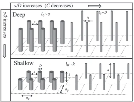
available for a large range of macro-roughness arrangement. Unlike cases involving vegetation, k/D for macro-roughness is close to one. As a result, the influence of the bed is greater when the obstacles are shallow.Figure 8shows the different possible configurations for each of the three length scales: s, k and D. To determine experimentally l0, the flow rate by

integrating the calculated vertical velocity proﬁle (steps 3c, 3d and 3e) is compared to the measured ﬂow rate with an

C

(a) (b) 0.05 0.1 0.15 0.2 0.25 0.3 0.35 0.4

f

C

(C

)

0 0.2 0.4 0.6 0.8 1 1.2 _(V/V g)2, ay/ax= 1 (V/Vg)2, ay/ax= 2 (V/Vg)2, ay/ax= 0.5 Nepf(1999), ay/ax= 1 Nepf(1999), ay/ax= 2 Nepf(1999), ay/ax= 0.5 Cassan et al. (2014)

C

0.05 0.1 0.15 0.2 0.25 0.3 0.35 0.4

f

C

(C

)

0 0.2 0.4 0.6 0.8 1 1.2 (V /Vg)2, ay/ax= 1 (V /Vg)2, ay/ax= 2 (V /Vg)2, ay/ax= 0.5 IdelCik, ay/ax= 1 IdelCik, ay/ax= 2 IdelCik, ay/ax= 0.5

Fig. 5. Measured corrective function as a function of concentration com-pared with formula ofNepf (1999) (a) andIdelcick (1986)(b).

F

0 0.5 1 1.5 2

f

F

(F

)

0 0.5 1 1.5 2 2.5 3 3.5 C = 0.19, ay/ax= 1 C = 0.095, ay/ax= 2 C = 0.10, ay/ax= 1 C = 0.05, ay/ax= 2 C = 0.08, ay/ax= 1.27 C = 0.13, ay/ax= 1.33 C = 0.19, ay/ax= 0.54 Cassan et al. (2014) R² = 0.20

h*

5 4 3 2 1 0

f

h*

(h

*

)

0 1 2 3 4 5 C = 0.19, ay/ax= 1 C = 0.095, ay/ax= 2 C = 0.10, ay/ax= 1 C = 0.05, ay/ax= 2 C = 0.08, ay/ax= 1.27 C = 0.13, ay/ax= 1.33 C = 0.19, ay/ax= 0.54 Cassan et al. (2014) R² = 0.23 (a) (b)

Fig. 6. Measured corrective function as a function of Froude number (a) and dimensionless water depth (b).

f

0

0.5

1

1.5

2 V

g

(m/s

)

0

1

2

3

4 h = 0.3 m, C=0.13

h = 0.6 m, C=0.13

h = 0.3 m, C=0.2

h = 0.6 m, C=0.2

Fig. 7. Velocity between blocks as a function of the ratio ax/ay.

Computation for a real scale ﬁshway (S = 0.05, D = 0.4 m, ks= 0.1 m,

(8)

optimization method (simplex algorithm from Matlab). For all experiments from literature (Kouwen and Unny, 1969;Meijer and Velzen, 1999; Lopez and Garcia, 2001; Righetti and Armanini, 2002;Poggi et al., 2004;Jarvela, 2005;Ghisalberti and Nepf, 2006;Murphy and Nepf, 2007;Kubrak et al., 2008;

Nezu and Sanjou, 2008;Huai et al., 2009;Yang and Choi, 2009;

Florens et al., 2013), Cdis considered equal to 1 if the block is

circular and Cd= 2 otherwise. The results performed byPoggi

et al. (2009),Konings et al. (2012),Nezu and Sanjou (2008),

Yang and Choi (2009),Huai et al. (2009), andKubrak et al. (2008)are reused, together with those obtained speciﬁcally for the present study. As indicated byKonings et al. (2012), the experiments carried out with leafy vegetation behaved in a

particular way because of viscosity terms. The interpretation of l0

is based on the assumptions ofBelcher et al. (2003)andKing et al. (2012). As expected, the experimental values of l0(Fig. 9)

are similar to s when s/k ≪ 1, and proportional to k when s/k> 0.15 which yields to equation(11).

Equation (11) is consistent with literature for shallow cases (Coceal and Belcher, 2004;Nikora et al., 2013) or for deep cases (Ghisalberti and Nepf, 2006;Luhar et al., 2008;

Huai et al., 2009; Poggi et al., 2009). For all experiments considered, the averaged error between the experimental and computed (with equation (11)) discharge is about 20% as indicated by the dashlines inFigure 9b. For the experiments performed in this study, the averaged error is 15.8%. Fig. 8. Deﬁnition of lengths and turbulent length scale (l0) as a function of blocks arrangement.

(a) Turbulent scale determined by comparing cal-culated and experimental discharge.

(b) Comparison of flow rates calculated with the model and measured flow rates per unit width. Dash lines represent error superior to

20%. R2_=0.93.

Fig. 9. Vegetation studies used to evaluate the model. Data fromLopez and Garcia (2001),Poggi et al. (2004),Meijer and Velzen (1999), Ghisalberti and Nepf (2006),Murphy and Nepf (2007),Nezu and Sanjou (2008),Yang and Choi (2009),Kubrak et al. (2008),Jarvela (2005), Kouwen and Unny (1969),Florens et al. (2013),Huai et al. (2009),Righetti and Armanini (2002).

Page 7 of10

(9)

3.3 Model validation

Lastly, the model is compared to the experimental correlation proposed byLarinier et al. (2006b)for rock-ramp ﬁsh passes (Eqs.(15)and(16)). This correlation is deduced from a statistical study of a large number of experiments in the laboratory, on cylindrical macro-roughness with 8 %< C < 16%, 1 %< S < 9%, k = 0.07 or 0.1 m and D = 0.035 m, the maximum ratio for h/k is 3.6.

For emergent conditions: q¼ 0:815 ffiffiffiffiffi gS p h D # $1:45 C!0:456D1:5: ð15Þ

For submerged conditions: q¼ 1:12 ffiffiffiffiffi gS p h D # $2:282 C!0:255 k D # $!0:799 D1:5: ð16Þ The experimental correlation of Pagliara et al. (2008) is also used (for emergent and submerged conditions):

q¼ Vh ¼ ffiffiffiffiffiffiffiffiffiffiffiffiffiffiffiffiffiffiffiffiffiffiffiffiffiffiffiffiffiffiffiffiffiffiffiffiffiffiffiffiffiffiffiffiffiffiffiffiffiffiffiffiffiffiffiffiffiffiffiffiffiffiffiffiffiffiffiffiffiffiffiffiffiffiffiffiffiffiffiffiffiffiffiffiffiffiffiffiffiffiffiffiffi 8ghS ð!7:82S þ 3:04Þð1:4 exp ð!2:98CÞ þ ln ðh=kÞÞ s h: ð17Þ The model results are consistent with the formula of

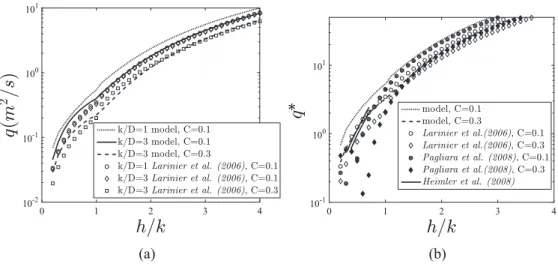
Larinier et al. (2006b), including high concentrations (Fig. 10) superior to C = 0.2. However the model differs from statistical formulation for low value of k/D. Experimental data with k/ D< 1 are used to calibrate the turbulence model whereas no such of experiments were used to establish the experimental correlation inLarinier et al.’s (2006)study. Similarly, equation

(16)indicates that D has no inﬂuence except for C because only one diameter was used. In the presented model, D modiﬁes the values of Cd, u0, s and then l0for deep cases. In

Figure 10, the stage-discharge relationship is depicted for a real scale ﬁshway. Comparison with other guidelines (Larinier et al., 2006b; Heimerl et al., 2008) indicates that the model allows to reproducing experimental correlation between h*and

q*= q/D5/2. The same dependence on C is found between the

present study and results of Pagliara et al. (2008). For emergent performance, the model with high concentration C = 0.3 provides the same stage-discharge relationship than method from Heimerl et al. (2008). Therefore, the model is validated by other studies. But, as mentioned before, some advantages are added like the applicability to different shapes and the validity for a large range of geometry.

Moreover, the model allows estimating the double averaged velocity proﬁle (Fig. 4) and turbulent shear stress (Eq.(7)) within and above the block layer whereas equations

(16)and(17)only provide the total discharge. It is possible to know if hydrodynamic parameters are suitable with the swimming ability of ﬁshes within the block layer even if the velocity is higher in the surface layer.

4 Conclusion

This paper presents an analytical model for calculating the stage-discharge relationship for emergent and submerged rock-ramp fish passes. New experiments are conducted to prove that results obtained byCassan et al. (2014)are available whatever the block arrangement. For submerged blocks, canopy vegetation models are improved to take mixing length into account by linking it directly to the geometric character-istics of the arrangement. The model has been adjusted on the basis of a large number of experiments found in the literature as well as the presented fish passes configurations. The model seems to offer a good trade-off between its validity for a large range of geometrical arrangements and simplicity of use (number of parameters, calculation time, etc.). Although the mixing-length model provides few explanations about the structure of the turbulence, it can be used to estimate mean flow rate between and above the blocks fairly accurately. It is thus possible to predict the velocities that the different species of fish will need to overcome. It can also help to design effective and durable passes. The implementation of the model could be difficult but all equations can be solved with numerical tools. Software is developed currently and its ergonomy has been designed to help to use the presented flow chart.

h/k

4 3 2 1 (a) (b) 0

q(

m

2

/s

)

10-2 10-1 100 101 k/D=1 model, C=0.1 k/D=3 model, C=0.1 k/D=3 model, C=0.3 k/D=1 Larinier et al. (2006), C=0.1 k/D=3 Larinier et al. (2006), C=0.1 k/D=3 Larinier et al. (2006), C=0.3

h/k

4 3 2 1 0

q*

10-1 100 101 model, C=0.1 model, C=0.3 Larinier et al.(2006), C=0.1 Larinier et al.(2006), C=0.3 Pagliara et al. (2008), C=0.1 Pagliara et al.(2008), C=0.3 Heimler et al. (2008)

Fig. 10. Comparison of the stage-discharge relationship between the model and the empirical formula ofLarinier et al. (2006b)(a) as a function of concentration and formula ofLarinier et al. (2006b),Heimerl et al. (2008)andPagliara et al. (2008)with k/D = 1 (b). Computation for a real scale ﬁshway (S = 0.05, D = 0.4 m, ks= 0.1 m, Cd0= 1).

(10)

Supplementary Material

The Supplementary Material is available at http://www. kmae-journal.org/10.1051/kmae/2016032/olm.

Acknowledgments. The research was supported by the ONEMA under the grant “Caractérisation des conditions hydrodynamiques dans les écoulements à fortes rugosités émergentes ou peu submergées”. This financial support is greatly appreciated.

NOTATIONS

a:ratio of the area where the bed friction occurs on ax" ay

at:turbulent length scale (m) within the blocks layer

b:force ratio between drag and turbulent stress k:von Karman’s constant

l:frontal density

s:ratio between the block area in the x, y plane and D2 j:dimensionless square of the velocity

ax:width of a cell (perpendicular to ﬂow) (m)

ay:length of a cell (parallel to ﬂow) (m)

C :blocks concentration

Cd0 : drag coefﬁcient of a block considering a single block

inﬁnitely high with F ≪ 1

Cd:drag coefﬁcient of a block under the actual ﬂow conditions

Cf:bed-friction coefﬁcient

d :zero-plane displacement of the logarithmic proﬁle (m) D :characteristic width facing the ﬂow (m)

F :Froude number based on h and Vg

F0:Froude number based on h and V

g :gravitational constant (m s!2) h :mean water depth in a cell (m) h*:dimensionless water depth (h/D)

k :height of blocks (m) ks:height of roughness (m)

l0:turbulent length scale (m) at the top of blocks (m)

N :ratio between bed friction force and drag force q :speciﬁc discharge per unit width (m2s!1) q*:speciﬁc discharge per unit width (m!0.5s!1)

Re :Reynolds number based on k and u0

R2:determination coefﬁcient

s :minimum distance between blocks S :bed slope

u :averaged velocity at a given vertical position (m s!1) u0:averaged velocity at the bed (m s!1)

uk:averaged velocity at the top of blocks (m s!1)

u*:shear velocity (m s!1)

Vg : averaged velocity in the section between two blocks

(m s!1)

V :bulk velocity (m s!1) z :vertical position (m) z0:hydraulic roughness (m)

~z :dimensionless vertical position

References

Baki A, Zhu D, Rajaratnam N. 2014. Mean ﬂow characteristics in a rock-ramp-type ﬁsh pass. J Hydraul Eng 140 (2): 156–168. Belcher SE, Jerram N, Hunt JCR. 2003. Adjustment of a turbulent

boundary layer to a canopy of roughness elements. J Fluid Mech 488: 369–398.

Cassan L, Tien T, Courret D, Laurens P, Dartus D. 2014. Hydraulic resistance of emergent macroroughness at large Froude numbers: design of nature-like ﬁshpasses. J Hydraul Eng 140 (9): 04014043.

Coceal O, Belcher SE. 2004. A canopy model of mean winds through urban areas. Q J R Meteorol Soc 130 (599): 1349–1372. Deﬁna A, Bixio A. 2005. Mean ﬂow turbulence in vegetated open

channel ﬂow. Water Resour Res 41: 1–12.

FAO. 2002. Fish passes – design, dimensions and monitoring. Rome: FAO, 138 p.

Florens E, Eiff O, Moulin F. 2013. Deﬁning the roughness sublayer and its turbulence statistics. Exp Fluids 54 (4): 1–15.

Ghisalberti M, Nepf HM. 2006. The structure of the shear layer in ﬂows over rigid and ﬂexible canopies. Environ Fluid Mech 6: 277–301.

Heimerl S, Krueger F, Wurster H. 2008. Dimensioning of ﬁsh passage structures with perturbation boulders. Hydrobiologia 609 (1): 197–204.

Huai W-x, Chen Z-b, Han J, Zhang L-x, Zeng Y-h. 2009. Mathematical model for the ﬂow with submerged and emerged rigid vegetation. J Hydrodyn B 21 (5): 722–729.

Huthoff F, Augustijn DCM, Hulscher SJMH. 2007. Analytical solution of the depth-averaged ﬂow velocity in case of submerged rigid cylindrical vegetation. Water Resour Res 43 (6): W06413 Idelcick IE. 1986. Mémento des pertes de charges. 3e édition.

Eyrolles, EDF.

Jarvela J. 2005. Effect of submerged ﬂexible vegetation on ﬂow structure and resistance. J Hydrol 307 (1–4): 233–241.

Katul GG, Poggi D, Ridolfi L. 2011. A flow resistance model for assessing the impact of vegetation on flood routing mechanics. Water Resour Res 47 (8): 1–15.

King AT, Tinoco RO, Cowen EA. 2012. A k-e turbulence model based on the scales of vertical shear and stem wakes valid for emergent and submerged vegetated ﬂows. J Fluid Mech 701: 1–39. Klopstra D, Barneveld H, van Noortwijk J, van Velzen E. 1997. Analytical model for hydraulic resistance of submerged vegetation. In: Proceedings of the 27th IAHR Congress, pp. 775–780. Konings AG, Katul GG, Thompson SE. 2012. A phenomenological

model for the ﬂow resistance over submerged vegetation. Water Resour Res 48 (2).

Kouwen N, Unny TE. 1969. Flow retardance in vegetated channels. J Irrigat Drain Div 95 (2): 329–344.

Kubrak E, Kubrak J, Rowinski PM. 2008. Vertical velocity distributions through and above submerged, ﬂexible vegetation. Hydrol Sci J 53 (4): 905–920.

Larinier M, Travade F, Porcher JP. 2006. Fishways: biological basis, design criteria and monitoring. Bull Fr Peche Piscic 364 (Suppl.): 208 p. ISBN 92-5-104665-4.

Larinier M, Courret D, Gomes P. 2006. Technical Guide to the Concept on nature-like Fishways. Rapport GHAAPPE RA.06.05-V1, 5 (in French).

Lopez F, Garcia M. 2001. Mean ﬂow and turbulence structure of open-channel ﬂow through non-emergent vegetation. J Hydraul Eng 127 (5): 392–402.

Page 9 of10

(11)

Luhar M, Rominger J, Nepf H. 2008. Interaction between ﬂow, transport and vegetation spatial structure. Environ Fluid Mech 8: 423–439.

Meijer DG, Velzen EHV. 1999. Prototype scale ﬂume experiments on hydraulic roughness of submerged vegetation. In: 28th International Conference, Int. Assoc. of Hydraul. Eng. and Res., Graz, Austria.

Murphy EG, Nepf H. 2007. Model and laboratory study of dispersion in ﬂows with submerged vegetation. Water Resour Res 43 (5): 1–12.

Nepf HM. 1999. Drag, turbulence, and diffusion in ﬂow through emergent vegetation. Water Resour Res 35 (2): 479–489. Nepf HM. 2012. Hydrodynamics of vegetated channels. J Hydraul

Res 50 (3): 262–279.

Nezu I, Sanjou M. 2008. Turbulence structure and coherent motion in vegetated canopy open-channel ﬂows. J Hydro-Environ Res 2 (2): 62–90.

Nikora N, Nikora V, O’Donoghue T. 2013. Velocity proﬁles in vegetated open-channel ﬂows: combined effects of multiple mechanisms. J Hydraul Eng 139 (10): 1021–1032.

Nikora V, Goring D, McEwan I, Grifﬁths G. 2001. Spatially averaged open-channel ﬂow over rough bed. J Hydraul Eng 127 (2): 123–133.

Pagliara S, Das R, Carnacina I. 2008. Flow resistance in large-scale roughness conditions. Can J Civil Eng 35: 1285–1293.

Poggi D, Krug C, Katul GG. 2009. Hydraulic resistance of submerged rigid vegetation derived from ﬁrst-order closure models. Water Resour Res 45 (10).

Poggi D, Porporato A, Ridolﬁ L. 2004. The effect of vegetation density on canopy sub-layer turbulence. Bound-Layer Meteorol 111: 565–587.

Rice C, Kadavy K, Robinson K. 1998. Roughness of loose rock riprap on steep slopes. J Hydraul Eng 124 (2): 179–185.

Righetti M, Armanini A. 2002. Flow resistance in open channel ﬂows with sparsely distributed bushes. J Hydrol 269 (1–2): 55–64.

Shimizu Y, Tsujimoto T. 1994. Numerical analysis of turbulent open-channel ﬂow over vegetation layer using a k-e turbulence model. J Hydrosc Hydraul Eng 11 (2): 57–67.

Tran DT. 2015. Metrologie et modelisation des ecoulements a forte pente autour d’obstacles: application au dimensionnement des passes naturelles, Ph.D. thesis, INPT (in French).

Yang W, Choi S-U. 2009. Impact of stem flexibility on mean flow and turbulence structure in depth-limited open channel flows with submerged vegetation. J Hydraul Res 47 (4): 445–454.

Cite this article as: Cassan L, Laurens P. 2016. Design of emergent and submerged rock-ramp ﬁsh passes. Knowl. Manag. Aquat. Ecosyst., 417, 45.