This is an author-deposited version published in : http://oatao.univ-toulouse.fr/
Eprints ID : 5623
To link to this article : DOI: 10.1109/TIP.2012.2187668
URL : http://dx.doi.org/
10.1109/TIP.2012.2187668
O
pen
A
rchive
T
OULOUSE
A
rchive
O
uverte (
OATAO
)
OATAO is an open access repository that collects the work of Toulouse researchers and
makes it freely available over the web where possible.
To cite this version :
Altmann, Yoann and Halimi, Abderrahim and Dobigeon, Nicolas
and Tourneret, Jean-Yves
Supervised nonlinear spectral unmixing
using a post-nonlinear mixing model for hyperspectral imagery
.
(2012) IEEE Transactions on Image Processing, vol. 21 (n° 6)
. pp.
3017-3025. ISSN 1057-7149
Any correspondence concerning this service should be sent to the repository
administrator: [email protected]
Supervised Nonlinear Spectral Unmixing Using
a Postnonlinear Mixing Model for
Hyperspectral Imagery
Yoann Altmann, Student Member, IEEE, Abderrahim Halimi, Student Member, IEEE,
Nicolas Dobigeon, Member, IEEE, and Jean-Yves Tourneret, Senior Member, IEEE
Abstract—This paper presents a nonlinear mixing model for hy-perspectral image unmixing. The proposed model assumes that the pixel reflectances are nonlinear functions of pure spectral compo-nents contaminated by an additive white Gaussian noise. These nonlinear functions are approximated using polynomial functions leading to a polynomial postnonlinear mixing model. A Bayesian algorithm and optimization methods are proposed to estimate the parameters involved in the model. The performance of the un-mixing strategies is evaluated by simulations conducted on syn-thetic and real data.
Index Terms—Hyperspectral imagery, postnonlinear model, spectral unmixing (SU).
I. INTRODUCTION
S
PECTRAL UNMIXING (SU) is one of the major issues when analyzing hyperspectral images. SU consists of iden-tifying the macroscopic materials present in an hyperspectral image and quantifying the proportions of these materials in the image pixels. Most SU strategies assume that pixel reflectances are linear combinations of pure component spectra [1]–[5]. The resulting linear mixing model (LMM) has been widely used in the literature and has provided interesting results. However, as explained in [6], the LMM can be inappropriate for some hyperspectral images, such as those containing sand, trees, or vegetation areas. Nonlinear mixing models provide an inter-esting alternative for overcoming the inherent limitations of the LMM. They have been proposed in the hyperspectral image literature for specific kinds of nonlinearities. More precisely, the bidirectional reflectance-based model proposed in [7] has been introduced for hyperspectral images including intimate mixtures. Conversely, the bilinear models recently studied in [8]–[11] address the problem of scattering effects, mainly observed in vegetation areas. Other more flexible unmixing techniques have been also proposed to handle a wider class of nonlinearity, including radial basis function networks [12], [13]The authors are with the University of Toulouse, IRIT/INP-EN-SEEIHT/TeSA, BP 7122, 31071 Toulouse cedex 7, France (e-mail: [email protected]; [email protected]; [email protected]; [email protected]).
Digital Object Identifier 10.1109/TIP.2012.2187668
and kernel-based models [14], [15]. This paper considers a class of nonlinear mixing models referred to as postnonlinear mixing
models (PNMMs). PNMMs are flexible generalizations of the
standard LMMs that have been introduced in [16] and [17] for source separation problems. The main advantage of PNMMs is that they can accurately model many different nonlinearities (as will be shown in this paper). This paper addresses the problem of supervised SU of hyperspectral images using PNMMs. Note that “supervised” means that the endmembers contained in the image have been estimated by an endmember extraction algorithm (EEA). As a consequence, the only parameters to be estimated are the abundances and the nonlinearity coefficients for all pixels of the image. In the last decades, many EEAs have been developed to identify the pure spectral components contained in a hyperspectral image (the reader is invited to consult [18] for a recent review of these methods). Most EEAs implicitly rely on the LMM and might be inappropriate for nonlinear models such as PNMMs. However, as noticed in [6], geometric EEAs are still adapted to identify endmembers and can be reasonably employed when the mixing model involves nonlinearities. Therefore, this paper proposes to extract the endmembers contained in the hyperspectral image using a geo-metric EEA, known as vertex component analysis (VCA) [19]. The recent nonlinear EEA introduced in [20] is also considered. Once the endmembers have been extracted from the image, we propose to estimate the abundances and the nonlinearity parameters involved in the PNMM using estimation algorithms based on Bayesian and least-square (LS) methods.
In the Bayesian framework, appropriate prior distributions are chosen for the unknown PNMM parameters. The joint pos-terior distribution of these parameters is then derived. However, the classical Bayesian estimators cannot be easily computed from this joint posterior. To alleviate this problem, a Markov-chain Monte Carlo (MCMC) method is used to generate sam-ples according to the posterior of interest. As in any Bayesian algorithm, the joint posterior distribution can be also used to compute confidence intervals for the parameter estimates. How-ever, the resulting computational complexity can be too heavy for practical applications. In order to reduce this computational complexity, we propose to study LS methods that have already received considerable attention in the hyperspectral imagery [2], [10], [14]. A first method based on Taylor series expansions is proposed to iteratively solve the LS criterion associated with the PNMM observation model. The Taylor approximations allow quadratic optimization problems to be solved at each iteration.
A second approach is based on a classical gradient method ded-icated to constrained problems.
This paper is organized as follows: Section II introduces the PNMM for hyperspectral image analysis. Section III presents a Bayesian unmixing algorithm associated with the proposed PNMM. Section IV studies the two alternative unmixing algo-rithms based on LS methods. Some simulation results conducted on synthetic and real data are shown and discussed in Section V. Conclusions are finally reported in Section VI.
II. POLYNOMIALPNMM
This section defines the nonlinear mixing model used for hy-perspectral image SU. More precisely, the -spectrum
of a mixed pixel is defined as a nonlinear trans-formation of a linear mixture of spectra contaminated by additive noise, i.e.,
(1)
where is the spectrum of the th ma-terial present in the scene, is its corresponding proportion, is the number of endmembers contained in the image, and is an appropriate nonlinear function. Moreover, is the number of spectral bands, and is an additive independent and identi-cally distributed zero-mean Gaussian noise sequence with vari-ance , denoted as , where is the identity matrix. Note that the usual matrix and vector notations
and have been used in
the right-hand side of (1).
The choice of an appropriate nonlinearity deserves a specific attention. Polynomials, sigmoids, and combinations of polynomial and sigmoidal nonlinearities have shown inter-esting properties for source separation [17]. This paper focuses on second-order polynomial nonlinearities defined by
(2) with . An interesting property of the resulting nonlinear model referred to as polynomial PNMM (PPNMM) is that it reduces to the classical LMM for . Thus, we can expect unmixing results at least as good as those presented in [21] and [2] where Bayesian and LS methods were investi-gated. Another motivation for using the PPNMM is the Weier-strass approximation theorem, which states that any continuous function defined on a bounded interval can be uniformly ap-proximated by a polynomial with any desired precision [22, p. 15]. As explained in [9], it is reasonable to consider polynomials with first- and second-order terms (since higher order terms can generally be neglected), which leads to (2). Higher order terms could be considered in the presence of more than two reflec-tions. However, the resulting interaction spectra are, in prac-tice, of low amplitude and are hardly distinguishable from the noise. Straightforward computations allow the PPNMM obser-vation vector (for a given pixel of the image) to be expressed as follows:
(3)
where denotes the Hadamard (term-by-term) product. Note that the resulting PPNMM includes bilinear terms such as those considered in [8]–[11]. However, the nonlinear terms are char-acterized by a single amplitude parameter , leading to a less complex model when compared with the models introduced in [8], [9], and [11]. Note that endmember (contained in ) can be obtained in the noise free case by setting
and in (3).
Due to physical considerations, the abundance vector sat-isfy the following positivity and sum-to-one constraints:
(4)
It is straightforward to show that the function is noninjective for a fixed . However, the unmixing problem is identifiable since the application
is injective under specific conditions related to the pure compo-nent spectra (see [23] for details).
III. BAYESIANESTIMATION
This section generalizes the hierarchical Bayesian model in-troduced in [21] to the PPNMM. The unknown parameter vector associated with the PPNMM contains the pixel abundances [satisfying constraints (4)], the nonlinearity parameter , and the additive noise variance . This section summarizes the likeli-hood and the parameter priors associated with the proposed hi-erarchical Bayesian PPNMM.
A. Likelihood
Equation (3) shows that , , are distributed according to a Gaussian distribution with mean and covariance
matrix (denoted as , , ). As
a consequence, the likelihood function of the observation vector can be expressed as
(5)
where is the standard norm.
B. Parameter Priors
In order to satisfy the sum-to-one constraint, the abundance vector can be rewritten1 with
and where notation indicates that the th com-ponent of has been removed, i.e., . The positivity constraints in (4) impose that belongs to the following simplex
(6)
1Note that the proposed parameterization is chosen for notation simplicity.
A uniform prior distribution on is chosen for to reflect the absence of prior knowledge about the abundance vector. A Jeffreys prior is chosen for
(7) which also reflects the absence of knowledge for this param-eter (see [24] for details). A conjugate Gaussian prior is finally chosen for the nonlinearity parameter , i.e.,
(8) The Gaussian prior is zero mean since the value of can be equally likely positive or negative. Moreover, it favors small values of and is a conjugate prior for parameter , which will simplify the computations.
C. Hyperparameter Prior
The hyperparameter is also included within the Bayesian model. A conjugate inverse-gamma prior is assigned to
(9) where are fixed to obtain a flat prior, reflecting the absence of knowledge about variance [ will be set to (1, ) in the simulation section].
D. Posterior Distribution of
The joint posterior distribution of the unknown parameter vector can be computed using the fol-lowing hierarchical structure:
(10) where means “proportional to” and is defined in (5). By assuming that parameters , , and are a priori inde-pendent, the joint prior distribution of the unknown parameter vector can be expressed as
(11) The joint posterior distribution can then be computed up to a multiplicative constant, i.e.,
(12) Unfortunately, it is difficult to obtain closed form expressions of the standard Bayesian estimators [including the maximum a
posteriori (MAP) and the minimum mean square error (MMSE)
estimators] associated with (12). The last part of this section studies an MCMC method that can be used to generate samples asymptotically distributed according to (12). These generated samples are then used to compute the MAP or MMSE estimators of the unknown parameter vector .
E. Metropolis-Within-Gibbs Sampler
The principle of the Gibbs sampler is to sample according to the conditional distributions of the posterior of interest [25, Chap. 10]. The probability density functions (pdf) associated with (12) are studied below.
1) Conditional pdf : Straightforward
computa-tions lead to
(13) where . Since it is not easy to sample according to (13) [mainly because of the indicator function ], we propose to update the abundance using a Metropolis–Hasting move. More precisely, a new abundance coefficient is proposed following a Gaussian random walk procedure (the variance of the proposal distribution has been adjusted to obtain an accep-tance rate close to 0.5, as recommended in [26, p. 8]). The gener-ated abundance is accepted or rejected with an appropriate prob-ability provided in Algorithm 1.
2) Conditional pdf : Using (5), it can be easily
shown that is distributed according to the following Gaussian distribution:
(14) where
and . As a consequence, sampling ac-cording to (14) is straightforward.
3) Conditional pdf : Looking carefully at (12),
it can be shown that , is distributed according to the following inverse-gamma distribution:
(15) from which it is easy to sample.
4) Conditional pdf : Finally, by looking at the
posterior distribution (12), it can be seen that , is dis-tributed according to the following inverse-gamma distribution: (16) The resulting Metropolis-within-Gibbs sampler used to sample according to (12) is summarized in Algorithm 1.
After generating samples using the procedures defined pre-viously, the MMSE estimator of the unknown parameters can be approximated by computing the empirical averages of these samples, after an appropriate burn-in period.2Even if the
sam-pling strategy has been observed to converge very fast, its com-putational complexity can be heavy for practical applications. The next section studies LS estimators, which allow this com-putational complexity to be significantly reduced.
2The length of the burn-in period has been determined using appropriate
IV. LS METHODS
LS methods have been successfully used for linear SU [2]. The LS method associated with the observation equation (3) consists of minimizing the following criterion:
(17) under the positivity and sum-to-one constraints (4). This opti-mization problem is not easy to handle mainly because of con-straints (4). However, the cost function is quadratic with respect to parameter . As a consequence, by differentiating with respect to , the following closed-form expression for can be obtained
(18)
After replacing (18) in , we obtain
(19)
where
(20)
We introduce below two strategies to compute the optimal abundance vector
under constraints (4). Note that, once has been computed, the nonlinearity parameter can be estimated as follows:
(21)
A. Taylor Approximation
Motivated by the method introduced in [10], we propose to approximate function defined in (20) using the first-order terms of a Taylor series expansion. Let denotes the esti-mated abundance vector estimate at the th iteration, and its corresponding estimated spectrum following (20). The Taylor approximation of at can be written
(22)
where is the gradient matrix of of size and is the unknown parameter vector to be estimated. The th column of can be derived from (3) as
where and the partial derivatives of and are available in [23]. Approximating in (19) using (22), vector can be estimated by solving the following con-strained LS problem:
(24) under constraints (4), where
(25) and is the gradient matrix. Problem (24) can be finally solved by the FCLS algorithm [2]. More pre-cisely, the sum-to-one constraint of the abundances is consid-ered by penalizing (24), leading to
(26) subject to the nonnegativity constraints for the parameter vector , where controls the impact of the sum-to-one constraint. Procedure (26) is repeated until convergence. The convergence of this iterative procedure to the global minimum of the objective function (21) is difficult to prove because of constraints (4) in (24). The next section introduces an alter-native subgradient-based algorithm whose convergence (to a local minimum of the associated objective function) is ensured.
B. Subgradient-Based Optimization
A gradient approach could be used to solve the cost func-tion defined in (19) in the absence of constraints. However, the problem is more complicated when constraints (4) have to be considered. The estimation method studied in this section is based on a subgradient optimization (SO) algorithm [27, p. 339] that is appropriate for constrained problems. More pre-cisely, subgradient-based optimization allows each abundance to be independently updated. Due to the sum-to-one constraint of the abundance vector, the cost function (19) can be expressed as a function of by setting . In that case, the cost function (19) can be rewritten as
(27) where
(28)
(29)
At a given point , the SO algorithm performs sequential line searches along directions defined by the partial deriva-tives with respect to (for ), i.e.,
where the partial derivatives of are provided in [23]. Finally, the line search procedure solves the following problem: (30)
where is a direction vector of
size , and (for
) are upper bounds for the line search parameters. More precisely, upper bounding according to the rule
if if if
ensures that constraints (4) are satisfied. Problem (30) can be solved using the golden section method [27, p. 270]. The abun-dances are then updated component by component (see [23] for more details about the algorithm). Here again, the procedure is repeated until convergence. The next section presents the per-formance of the proposed algorithms on synthetic and real hy-perspectral images.
V. SIMULATIONS
A. Synthetic Data
The performance of the proposed nonlinear SU algorithms is first evaluated by unmixing four synthetic images of size 50 50 pixels. The endmembers contained in these images have been extracted from the spectral libraries provided with the ENVI software [28] (i.e., green grass, olive-green paint, and galvanized steel metal). The first synthetic image has been generated using the standard LMM. A second image has been generated according to the bilinear mixing model introduced in [10], referred to as “Fan model” (FM). A third image has been generated according to the generalized bilinear mixing model (GBM) presented in [11], whereas a fourth image has been generated according to the PNMM. For each image, the abun-dance vectors , , have been randomly gen-erated according to a uniform distribution over the admissible set defined by the positivity and sum-to-one constraints. All im-ages have been corrupted by an additive white Gaussian noise of variance , corresponding to a signal-to-noise ratio SNR dB. The nonlinearity co-efficients are uniformly drawn in the set (0, 1) for the GBM, and parameter has been uniformly generated in the set ( 0.3, 0.3) for the PPNMM. Different estimation procedures have been considered for the four mixing models.
1) For the LMM, we have considered the standard FCLS al-gorithm [2] and the Bayesian alal-gorithm of [21].
2) The FM has been unmixed using the LS method introduced in [10] and a Bayesian algorithm similar to the one derived in [11] but assuming all the nonlinearity coefficients are equal to 1.
3) The unmixing strategies used for the GBM are the three algorithms presented in [29], i.e., a Bayesian algorithm and two LS methods.
TABLE I
ABUNDANCERMSES : SYNTHETICIMAGES
4) The Bayesian and LS algorithms presented in Sections III and IV have been used for unmixing the proposed PPNMM. Note that all results presented in this paper have been obtained using the Bayesian MMSE estimator. The quality of the unmixing procedures can be measured by comparing the estimated and actual abundance vector using the root mean square error (RMSE) defined by
RMSE (31)
where and are the actual and estimated abundance vec-tors for the th pixel of the image and is the number of image pixels. Table I shows the RMSEs associated with images for the different estimation procedures. Note that the best results (in terms of RMSE) for each image have been repre-sented in underlined bold, whereas the second best results have been depicted in bold. Table I shows that the abundances esti-mated by the Bayesian algorithm and the LS methods are similar for the PPNMM. Moreover, for these four images, the PPNMM seems to be more robust than the other mixing models to de-viations from the actual model. Indeed, the PPNMM provides small abundance RMSEs for the four images .
The unmixing quality can be also evaluated by the reconstruc-tion error (RE) defined as
RE (32)
where is the th observation vector and is its estimate. Table II compares the REs obtained for the different synthetic images. These results show that the REs are close for the different unmixing algorithms. Again, the proposed PPNMM seems to be more robust than the other mixing models to deviations from the actual model in terms of RE.
Fig. 1 shows the estimated distributions of for images using the three presented algorithms (i.e., Bayesian, linearization, and subgradient). This figure shows that the algo-rithms similarly perform for the estimation of the nonlinearity parameter .
Table III shows the execution times of MATLAB implemen-tations on a 1.66-GHz Dual Core of the proposed algorithms for unmixing the proposed images (2500 pixels for each image). The linearization-based algorithm has the lowest computational
TABLE II
RES : SYNTHETICIMAGES
Fig. 1. Histograms of the estimated nonlinearity parameter for the four syn-thetic images estimated by the (black) Bayesian, (red) linearization-based and (blue) subgradient-based algorithms.
TABLE III
COMPUTATIONALTIMES OF THEUNMIXINGALGORITHMS FOR2500 PIXELS
(INSECOND)
cost and also provides accurate estimations. Note that the com-putational cost of the Bayesian algorithm (which allows prior knowledge to be included in the unmixing procedure) can be prohibitive for larger images and a high number of endmembers. However, the computational cost of the two proposed optimiza-tion methods (linearizaoptimiza-tion and gradient based) is very reason-able, which make them very useful for practical applications.
The next set of simulations analyzes the performance of the proposed nonlinear SU algorithms for different numbers of end-members by unmixing four synthetic im-ages of 500 pixels. The endmembers contained in these imim-ages have been randomly selected from the 14 endmembers extracted by VCA from the full Cuprite scene described in [30]. For each image, the abundance vectors , , have been randomly generated according to a uniform distribution over the admissible set defined by the positivity and sum-to-one con-straints. All images have been corrupted by an additive white
TABLE IV
AVERAGERMSES : SYNTHETICIMAGES
TABLE V
AVERAGERES : SYNTHETICIMAGES
Gaussian noise corresponding to a signal-to-noise ratio SNR dB. The nonlinearity coefficient is uniformly drawn in the set ( 0.3, 0.3). Tables IV and V compare the performance of the three proposed methods in terms of abundance estimation and RE. These results show that the three methods similarly perform in terms of RE. The Bayesian estimators tend to provide more accurate abundance estimations (i.e., smaller RMSEs) for large values of . Indeed, the Taylor and gradient algorithms may be trapped in local minima of the LS criterion (17) for large values of .
B. Real Data
The first real image considered in this section is composed of spectral bands and was acquired in 1997 by the airborne visible infrared imaging spectrometer (AVIRIS) over the Cuprite mining site in Nevada. A subimage of size 50 50 pixels has been chosen here to evaluate the proposed unmixing procedures. The scene is mainly composed of muscovite, alu-nite, and kaolialu-nite, as explained in [31]. The endmembers ex-tracted by VCA [19] and the nonlinear EEA proposed in [20] (referred to as “Heylen”), with , are depicted in Fig. 2. The endmembers obtained by the two methods have similar shapes. This result confirms the fact that the geometric EEAs (such as VCA) can be used as a first approximation for end-member estimation [6]. The estimation algorithms presented in Sections III and IV have been applied to each pixel of the scene using the endmembers extracted by the two EEAs. Examples of abundance maps obtained for endmembers estimated using Heylen’s method are presented in Fig. 3 (see [23] for similar results obtained with endmembers estimated by VCA]. The ad-vantage of the PPNMM is that it allows the nonlinearities be-tween the observations and the abundance vectors to be ana-lyzed. For instance, Fig. 4 shows the estimated maps of for the Cuprite image. These results show that the observations are nonlinearly related to the endmembers (since ). However, the nonlinearity is weak since the estimated values of are close to 0.
The second real image considered in this section is composed of spectral bands and was acquired in 1997 by the satellite AVIRIS over the Moffett Field, CA. A subimage of size
Fig. 2. endmembers estimated by (blue lines) VCA and (red lines) Heylen for the Cuprite scene.
Fig. 3. Abundance maps estimated by the Bayesian, linearization, and subgra-dient methods for the Cuprite scene.
Fig. 4. Maps of the nonlinearity parameter estimated by the Bayesian, lin-earization, and subgradient methods for the Cuprite scene.
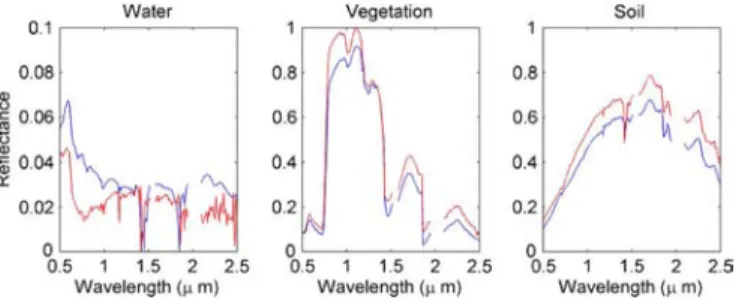
Fig. 5. endmembers estimated by (blue lines) VCA and (red lines) Heylen for the Moffett scene.
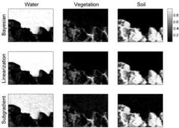
50 50 pixels has been also chosen here to evaluate the pro-posed unmixing procedures. The scene is mainly compro-posed of water, vegetation, and soil. The endmembers extracted by VCA and the Heylen’s method with are depicted in Fig. 5. Again, the endmembers obtained by the two methods are sim-ilar. Examples of abundance maps estimated by the proposed
Fig. 6. Abundance maps estimated by the Bayesian, linearization, and subgra-dient methods for the Moffett scene.
Fig. 7. Maps of the nonlinearity parameter estimated by the Bayesian, lin-earization, and subgradient methods for the Moffett scene.
TABLE VI
RES : CUPRITE ANDMOFFETTIMAGES
algorithms are presented in Fig. 6 (endmembers have been es-timated using Heylen’s method). They are similar to the abun-dance maps obtained with estimation algorithms associated with the LMM (available in [21]). Fig. 7 shows the estimated maps of for the Moffett image. In the water area, the observations are nonlinearly related to the endmembers (since ). These nonlinearities can be due to the low amplitude of the water spec-trum and possible nonlinear bathymetric effects.
The quality of unmixing is finally evaluated using the REs for both real images. These REs are compared in Table VI with those obtained by assuming other mixing models. The proposed PPNMM provides smaller REs when compared with other models, which is a very encouraging result. Additional results on the full Cuprite scene are available in [23].
VI. CONCLUSION ANDFUTUREWORKS
A Bayesian and two least squares algorithms were presented for nonlinear spectral unmixing of hyperspectral images. These algorithms assumed that the hyperspectral image pixels are re-lated to the endmembers by a polynomial post-nonlinear mixing model. In the Bayesian framework, the constraints related to the unknown parameters were ensured by using appropriate prior distributions. The posterior distribution of the unknown parameter vector was then derived. The corresponding min-imum mean square error estimator was approximated from samples generated using Markov chain Monte Carlo methods. Least squares methods were also investigated for unmixing the PPNMM. These methods provided results similar to the Bayesian algorithm with a reduced computational cost, making them very attractive for hyperspectral image unmixing. Results obtained on synthetic and real images illustrated the accuracy of the PPNMM and the performance of the corresponding esti-mation algorithms. Future works include the study of nonlinear EEAs appropriate for the proposed parametric PPNMM. De-riving nonlinearity detectors based on the proposed parametric PPNMM is also under investigation.
ACKNOWLEDGMENT
The authors would like to thank R. Heylen and P. Scheunders from University of Antwerp, Antwerp, Belgium, for supplying the Matlab codes related to the nonlinear endmember extraction algorithm studied in [20] and used in this paper.
REFERENCES
[1] M. Craig, “Minimum volume transforms for remotely sensed data,”
IEEE Trans. Geosci. Remote Sens., vol. 32, no. 3, pp. 542–552, May
1994.
[2] D. C. Heinz and C.-I. Chang, “Fully constrained least-squares linear spectral mixture analysis method for material quantification in hyper-spectral imagery,” IEEE Trans. Geosci. Remote Sens., vol. 39, no. 3, pp. 529–545, Mar. 2001.
[3] O. Eches, N. Dobigeon, C. Mailhes, and J.-Y. Tourneret, “Bayesian estimation of linear mixtures using the normal compositional model,”
IEEE Trans. Image Process., vol. 19, no. 6, pp. 1403–1413, Jun. 2010.
[4] L. Miao, H. Qi, and H. Szu, “A maximum entropy approach to unsuper-vised mixed-pixel decomposition,” IEEE Trans. Image Process., vol. 16, no. 4, pp. 1008–1021, Apr. 2007.
[5] Z. Yang, G. Zhou, S. Xie, S. Ding, J.-M. Yang, and J. Zhang, “Blind spectral unmixing based on sparse nonnegative matrix factorization,”
IEEE Trans. Image Process., vol. 20, no. 4, pp. 1112–1125, Apr. 2011.
[6] N. Keshava and J. F. Mustard, “Spectral unmixing,” IEEE Signal
Process. Mag., vol. 19, no. 1, pp. 44–57, Jan. 2002.
[7] B. W. Hapke, “Bidirectional reflectance spectroscopy. I. Theory,” J.
Geophys. Res., vol. 86, no. B4, pp. 3039–3054, Apr. 1981.
[8] B. Somers, K. Cools, S. Delalieux, J. Stuckens, D. V. der Zande, W. Verstraeten, and P. Coppin, “Nonlinear hyperspectral mixture analysis for tree cover estimates in orchards,” Remote Sens. Environ., vol. 113, no. 6, pp. 1183–1193, Jun. 2009.
[9] J. M. P. Nascimento and J. M. Bioucas-Dias, SPIE, “Nonlinear mix-ture model for hyperspectral unmixing,” in Proc. SPIE Image Signal
Process. Remote Sens. XV, L. Bruzzone, C. Notarnicola, and F. Posa,
Eds., 2009, vol. 7477, no. 1, p. 747 70I.
[10] W. Fan, B. Hu, J. Miller, and M. Li, “Comparative study between a new nonlinear model and common linear model for analysing laboratory simulated-forest hyperspectral data,” Remote Sens. Environ., vol. 30, no. 11, pp. 2951–2962, Jun. 2009.
[11] A. Halimi, Y. Altmann, N. Dobigeon, and J.-Y. Tourneret, “Nonlinear unmixing of hyperspectral images using a generalized bilinear model,”
IEEE Trans. Geosci. Remote Sens., vol. 49, no. 11, pp. 4153–4162,
[12] K. J. Guilfoyle, M. L. Althouse, and C.-I. Chang, “A quantitative and comparative analysis of linear and nonlinear spectral mixture models using radial basis function neural networks,” IEEE Geosci. Remote
Sens. Lett., vol. 39, no. 10, pp. 2314–2318, Oct. 2001.
[13] Y. Altmann, N. Dobigeon, S. McLaughlin, and J.-Y. Tourneret, “Non-linear unmixing of hyperspectral images using radial basis functions and orthogonal least squares,” in Proc. IEEE IGARSS Conf., Jul. 2011, pp. 1151–1154.
[14] J. Broadwater, R. Chellappa, A. Banerjee, and P. Burlina, “Kernel fully constrained least squares abundance estimates,” in Proc. IEEE IGARSS
Conf., Barcelona, Spain, 2007, pp. 4041–4044.
[15] K.-H. Liu, E. Wong, and C.-I. Chang, “Kernel-based linear spectral mixture analysis for hyperspectral image classification,” in Proc. IEEE
WHISPERS, Grenoble, France, Aug. 2009, pp. 1–4.
[16] C. Jutten and J. Karhunen, “Advances in nonlinear blind source separation,” in Proc. 4th Int. Symp. ICA, Nara, Japan, Apr. 2003, pp. 245–256.
[17] M. Babaie-Zadeh, C. Jutten, and K. Nayebi, “Separating convolutive post non-linear mixtures,” in Proc. 3rd ICA Workshop, San Diego, CA, 2001, pp. 138–143.
[18] M. Parente and A. Plaza, “Survey of geometric and statistical un-mixing algorithms for hyperspectral images,” in Proc. IEEE GRSS
WHISPERS, Reykjavıacute;k, Iceland, 2010.
[19] J. M. Nascimento and J. M. B. Dias, “Vertex component analysis: A fast algorithm to unmix hyperspectral data,” IEEE Trans. Geosci. Remote
Sens., vol. 43, no. 4, pp. 898–910, Apr. 2005.
[20] R. Heylen, D. Burazerovic, and P. Scheunders, “Non-linear spectral unmixing by geodesic simplex volume maximization,” IEEE J. Sel.
Topics Signal Process., vol. 5, no. 3, pp. 534–542, Jun. 2011.
[21] N. Dobigeon, J.-Y. Tourneret, and C.-I. Chang, “Semi-supervised linear spectral unmixing using a hierarchical Bayesian model for hyperspectral imagery,” IEEE Trans. Signal Process., vol. 56, no. 7, pp. 2684–2695, Jul. 2008.
[22] V. J. Mathews and G. L. Sicuranza, Polynomial Signal Processing. New York: Wiley, 2000.
[23] Y. Altmann, A. Halimi, N. Dobigeon, and J.-Y. Tourneret, “Supervised nonlinear spectral unmixing using a post-nonlinear mixing model for hyperspectral images,” Univ. Toulouse, Toulouse, France, Tech. Rep., Nov. 2011. [Online]. Available: http://altmann.perso.enseeiht.fr/ [24] E. Punskaya, C. Andrieu, A. Doucet, and W. Fitzgerald, “Bayesian
curve fitting using MCMC with applications to signal segmentation,”
IEEE Trans. Signal Process., vol. 50, no. 3, pp. 747–758, Mar. 2002.
[25] C. P. Robert and G. Casella, Monte Carlo Statistical Methods, 2nd ed. New York: Springer-Verlag, 2004.
[26] C. P. Robert and D. Cellier, “Convergence control of MCMC algo-rithms,” in Discretization and MCMC Convergence Assessment, C. P. Robert, Ed. New York: Springer-Verlag, 1998, pp. 27–46. [27] M. Bazaraa, H. Sherali, and C. Shetty, Nonlinear Programming:
Theory and Algorithms, 2nd ed. New York: Wiley, 1993. [28] “ENVI User’s Guide Version 4.0,” RSI, Boulder, CO, Sep. 2003. [29] A. Halimi, Y. Altmann, N. Dobigeon, and J.-Y. Tourneret, “Unmixing
hyperspectral images using a generalized bilinear model,” in Proc.
IEEE IGARSS Conf., Jul. 2011, pp. 1886–1889.
[30] R. N. Clark, G. A. Swayze, K. E. Livo, R. F. Kokaly, S. J. Sutley, J. B. Dalton, R. R. McDougal, and C. A. Gent, “Imaging spectroscopy: Earth and planetary remote sensing with the USGS Tetracorder and expert systems,” J. Geophys. Res., vol. 108, no. E12, pp. 5-1–5-44, Dec. 2003.
[31] N. Dobigeon, S. Moussaoui, M. Coulon, J.-Y. Tourneret, and A. O. Hero, “Joint Bayesian endmember extraction and linear unmixing for hyperspectral imagery,” IEEE Trans. Signal Process., vol. 57, no. 11, pp. 4355–4368, Nov. 2009.
Yoann Altmann (S’11) was born in Toulouse,
France, in 1987. He received the Eng. degree in electrical engineering from ENSEEIHT, Toulouse, and the M.Sc. degree in signal processing from the National Polytechnic Institute of Toulouse, Toulouse, both in June 2010. He is currently working toward the Ph.D. degree with the Signal and Com-munication Group, IRIT Laboratory, Toulouse.
Abderrahim Halimi (S’11) was born in Algiers,
Al-geria, in 1987. He received the Eng. degree in elec-tronics from the Nationale Polytechnic School of Al-giers, AlAl-giers, in 2009 and the M.Sc. degree in signal processing from the National Polytechnic Institute of Toulouse, Toulouse, France, in 2010. He is currently working toward the Ph.D. degree with the Signal and Communication Group, IRIT Laboratory, Toulouse.
Nicolas Dobigeon (S’05–M’08) was born in
An-goulême, France, in 1981. He received the Eng. degree in electrical engineering from ENSEEIHT, Toulouse, France, in 2004 and the M.Sc. and Ph.D. degrees in signal processing from the National Polytechnic Institute of Toulouse, Toulouse, in 2004 and 2007, respectively.
From 2007 to 2008, he was a Postdoctoral Re-search Associate with the Department of Electrical Engineering and Computer Science, University of Michigan, Ann Arbor. Since 2008, he has been an Assistant Professor with the National Polytechnic Institute of Toulouse (ENSEEIHT, University of Toulouse), within the Signal and Communication Group, IRIT Laboratory. His research interests are focused on statistical signal and image processing, with particular interest in Bayesian inference and Markov-chain Monte Carlo methods.
Jean-Yves Tourneret (SM’08) received the
In-génieur degree in electrical engineering from ENSEEIHT, Toulouse, France, in 1989 and the Ph.D. degree from the National Polytechnic Institute of Toulouse, Toulouse, in 1992.
He is currently a Professor with the University of Toulouse, Toulouse, and a member of the IRIT laboratory (UMR 5505 of the Centre National de la Recherche Scientifique). His research activities are centered on statistical signal processing, with partic-ular interest to Bayesian inference and Markov-chain Monte Carlo methods.
Dr. Tourneret was the program chair of the European Conference on Signal Processing held in Toulouse in 2002. He was also a member of the organizing committee for the International Conference on Acoustics, Speech, and Signal Processing 2006, which was held in Toulouse in 2006. He has been a member of different technical committees including the Signal Processing Theory and Methods committee of the IEEE Signal Processing Society (2001–2007 and 2010–present). He served as an associate editor for the IEEE TRANSACTIONS ONSIGNALPROCESSING(2008–2011).