This is an author-deposited version published in: http://oatao.univ-toulouse.fr/
Eprints ID: 8416
To link to this article: DOI: 10.1115/1.4023194
URL: http://dx.doi.org/10.1115/1.4023194
To cite this version: Volpe, Raffaele and Da-Silva, Arthur and Ferrand, Valérie and Le Moyne, Luis Experimental and Numerical Validation of a
Wind Gust Facility. (2013) Journal of Fluids Engineering, vol. 135 (n° 1).
ISSN 0098-2202
O
pen
A
rchive
T
oulouse
A
rchive
O
uverte (
OATAO
)
OATAO is an open access repository that collects the work of Toulouse researchers and makes it freely available over the web where possible.
Any correspondence concerning this service should be sent to the repository administrator: [email protected]
1
Experimental and numerical validation of a wind gust facility
VOLPE Raffaelea,*, DA SILVA Arthura, FERRAND Valérieb, LE MOYNE Luisa. a
Laboratoire DRIVE, Institut Supérieur de l'Automobile et des Transports, Université de Bourgogne, 49 rue Mademoiselle Bourgeois, 58000 Nevers, France
b
Université de Toulouse, Institut Supérieur de l'Aéronautique et de l'Espace (ISAE), 10 avenue Edouard Belin, 31400 Toulouse, France.
*
Telephone: +33 5 61 33 81 47, Mobile: +33 6 83 49 05 38, e-mail: [email protected]
Abstract
The study of a vehicle moving through a lateral wind gust has always been a difficult task, due to the difficulties in granting the right similitude. The facility proposed by Ryan and Dominy has been one of the best options to carry it out. In this approach, a double wind tunnel is used to send a lateral moving gust on a stationary model. Starting from this idea, the ISAE has built a dedicated test bench for lateral wind studies on transient conditions. An experimental work has been carried out by means of Time-Resolved PIV, aiming at studying the unsteady interpenetration of the two flows coming from each wind tunnel. Meanwhile, a 3D CFD model based on URANS was set up, faithfully reproducing the double wind tunnel. Both experimental and numerical results are compared, and the evolution of the reproduced wind gust is discussed. Conclusions are finally taken about the validity of this kind of test bench for ground vehicles applications.
Keywords: Fluid mechanics, vehicle aerodynamics, crosswind, unsteady aerodynamics, yaw angle, TR-PIV, 3D CFD
1 Introduction
2
One of the most studied research topics in vehicle design has been the reduction of the aerodynamic resistance. Current trends on CO2 emissions and the need for energy efficiency, along with growing concern for safety in transports under any situation, ask for deepened research on aerodynamic optimization. This led to the optimization of automotive wind tunnels and measurement techniques for steady state flow tests, leaving the transient effects understudied. However, in the last years, more and more importance is being given to the knowledge of a vehicle's aerodynamic behavior faced to a side unsteady flow, such as a wind gust.
For example, Hémon and Noger [1] set up a linearized quasi-steady model of vehicle dynamics in order to study the transient growth of energy phenomenon. They stated that energy amplification occurs when a vehicle is subjected to a steep change of wind direction, so that estimation of lateral stability should not simply rely on static data. As a matter of fact, the response of aerodynamic side force and yaw moment to a sudden change in lateral wind is not linear but can present transient effects that can lead to peaks of force, and so to a potential source of hazard for the driver's behavior [2; 3].
For many years it was thought that steady yaw wind tunnel tests could give enough information in the evaluation of the dynamic stability, even if already in 1967 Beauvais [4] showed that, when the yaw angle becomes greater than 15°, the yaw moment unsteady peak can be up to 20% greater than the same effort measured in steady state yawed condition.
Recently, several techniques have been conceived to study the evolution of aerodynamic coefficients to a time-dependent side wind. The first dynamical approach was displacing the model on a rail crossing the wind tunnel section [4-7]. Though nearly all the authors agree in estimating the unsteady force peak being 20 to 50% greater than the yawed vehicle steady force, little concordant results have been presented on the evolution of force as a function of time, especially when discussing the sudden wind direction change. Beauvais [4] states that aerodynamic forces reach their steady state condition after the
3
vehicle has covered 4 times its length in the gust, whereas for Cairns [5] and Chadwick [7] 5 vehicle lengths do not seem to be enough.
Another approach, extending the classical tests, consists of giving a periodic yaw angle to the model in a steady wind [8]. Even if low yaw angles and oscillation frequencies were tested, this kind of test bench carried out an interesting result: a phase angle difference is visible in drag force behavior, which means that there is a delay in the formation of the same drag between steady yaw angle tests and the corresponding dynamic yaw position. This was explained by Chometon et al. [9] using PIV measurements. It was found that vortex structures developing from the rear side do not adapt instantly to the new yawed position, but persist in the flow, as if they had a kind of “vortex inertia”. Both of the presented techniques, involving the vehicle motion, suffer from the presence of signal noise because of the vibrations induced by the moving facility, lowering the reliability of results. This noise heavily affects the measured signal, especially when using on-board balances, so that many identical tests are required and care must be taken when processing these data.
Due to these problems, experimental techniques using static vehicle models have become of interest. The most commonly used method is the estimation of the transient effects from the steady yaw coefficients and the wind spectral density by means of the aerodynamic admittance function [10], which can be measured once from high turbulence tests [11; 12] or with a device creating an oscillating flow upstream the vehicle [13; 14]. Despite being a reliable and well documented technique, it gives little information about the unsteady phenomena of the interaction between the gust and the vehicle. An approach possibly resolving this problem comes from Dominy [15]. His idea was to place a static vehicle model in a longitudinal flow. Then, a lateral moving gust was simulated by means of an auxiliary wind tunnel whose communication with the main flow is controlled via a sliding door. This experimental device has been reproduced differently like in Ryan’s [16] work, whose approach will be
4 reviewed in detail in this paper, in paragraph 2.1.
Along with expensive experiment tests, computational approaches have been developed, as presented in the next section.
1.2 Computational Fluid Dynamics approaches
Most of the simulations presented in literature regarding crosswind were validated simply on the basis of steady state yawed model experiments (mostly because of the lack of unsteady experimental data for the chosen vehicle), so particular care should be taken when generalizing these results. CFD simulations of vehicle motion, especially in presence of crosswind, still suffer from a lack of information in literature. This probably comes from the unavoidable use of sliding or deforming meshes, which can cause numerical convergence difficulties and unreliable results. As an example, Tsubokura et al. [17] tried to reproduce the yaw oscillating vehicle proposed by Garry and Cooper using a rotating grid. Even if some results could be processed, they presented important numerical irregularities caused by errors in calculation of the mass flow when the grid was changing.
In the commonly used approach, static grids are used. Firstly, the steady vehicle running condition is simulated, then unsteady boundary conditions reproduce the gust passage. This kind of modeling is actually the same as the experimental test bench proposed by Dominy.
Due to the high Reynolds numbers (varying from 105 to 106), DNS simulations are computationally expensive, so that turbulence modeling is needed. The classical models are DES and LES, combining both accuracy in calculation of turbulence high scales and a smaller computational effort.
Tsokubura et al. [18] used LES on a real car shape with this method and showed the evolution of aerodynamic force tensor for a stepwise gust presenting a 30° yaw angle change. The most important dynamic effects were the overshoot in the yaw angle and an undershoot in the drag force; it was also visible that the relaxation time for the three moments is longer than the imposed gust ramp and
5
corresponds to that of the lift force. The authors related this mostly to the evolution of pressure in the under-body, especially near the windward wheels. Favre [19] reproduced the effects of a moving trapezoidal shape gust on a simplified vehicle shape for different angles by DES. Tsubokura's results were confirmed and they showed how the pressure field evolves during the gust, suggesting that a square back geometry may be the better compromise between better fuel consumption and crosswind stability. Hemida and Krajnovic [20] also used DES for simulating a double deck bus exit from a tunnel to a windy bridge and found that potentially hazardous unsteady effects on the side force can be seen before the actual passage in the gust.
1.3 The objective of this work
In recent years, the ISAE in Toulouse (France) started working in the development of a test bench for the study of a wind gust by means of laser techniques. Relying on the literature presented in previous sections, it was decided to produce a double wind tunnel, on the idea by Dominy. In particular, a version of this device inspired by Ryan [16], in which the sliding door is replaced by a series of shutters, was adapted to an already existing wind tunnel. In this paper is presented the work concerning characterization of the gust produced by the new device in the measurement region. The main difference with Ryan's work is the use of an non-intrusive measurement technique such as the Time-Resolved Particle Image Velocimetry (TR-PIV), whereas he had to sample his test section using a hot-wire probe. In parallel, a numerical approach is presented with a 3D CFD model of the same test bench. This CFD simulation approach was also proposed by Ryan, but using a 2D modeling. Furthermore, Ryan’s geometry did not include a secondary wind tunnel, but a lateral inlet section of the computational domain with transient Dirichlet boundary conditions.
In the following, both experimental and numerical methods are described. In each case a double wind tunnel is set up and the wind gust penetration into the main steady state flow is reproduced by the
6
opening and closing sequence of a series of shutters placed in the auxiliary wind tunnel, before its intersection with the main tunnel.
2 Experimental set-up
2.1 Description of the “Rafale latérale” test bench at ISAE
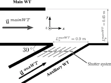
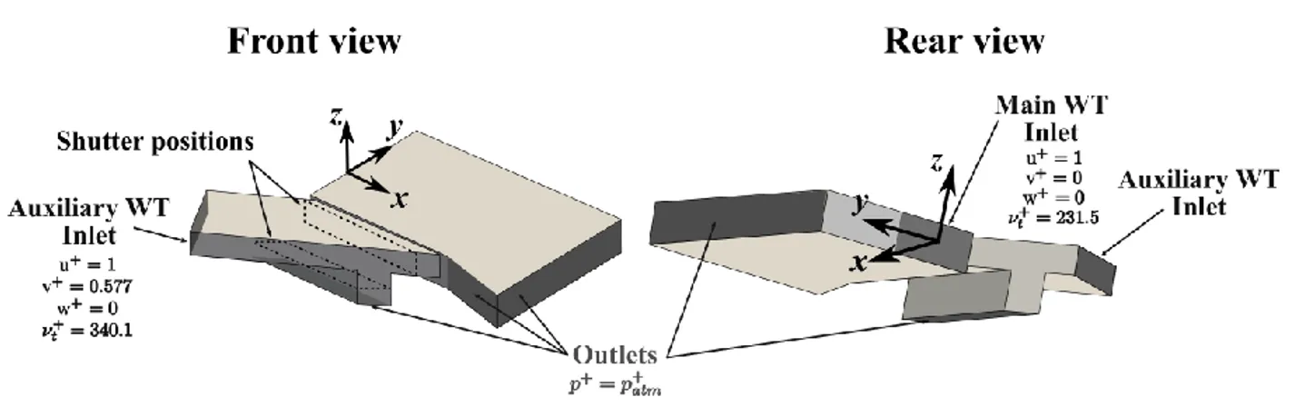
On the basis of the issues seen in the moving model experiments, the ISAE developed its own wind gust test bench as a stationary model facility. The inspiring idea was the one from Dominy and Docton [21] and then further developed by Ryan [16], in which the gust is simulated by introducing a side moving jet in the steady flow of a standard wind tunnel. This is achieved by means of an auxiliary wind tunnel whose communication is granted by a system of electrically driven shutters (Fig. 1-2).
Figure 1: Wind gust generator by use of an auxiliary wind tunnel.
Figure 2: CAD drawing of the ISAE testbench
The semi-enclosed test section dimensions are LmainWTy = 0.45 m, mainWT z
L = 0.21 m and LauxWTx = 0.90 m, auxWT
z
L = 0.15 m for the end section of the auxiliary wind tunnel. The height of the auxiliary wind tunnel is centered on the main wind tunnel section, as shown in Fig. 3. In the further tests, the car model will be fixed on a raised floor, aligned with the one of the auxiliary wind tunnel. This will allow us to uniform the main flow boundary layer profile at model position.
7
The relative angle is 30°: as seen by Macklin et al. [22], at this yaw angle occur the maximum values of yaw moment and side force in steady state experiments.
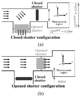
The interior of the auxiliary wind tunnel is divided in 20 channels, with a shutter in each of them controlling the air flow; every shutter can be opened and closed by means of an electromagnet – spring system, which can be driven remotely by a LabView interface. To ensure mass flow conservation through every channel whatever the number of open doors is, the auxiliary wind tunnel has a second exit whose opening is controlled by a twin row of shutters, Fig. 3. So, when the opening of a door is commanded, at the same time the twin door is closed.
Figure 3: Projected side view scheme of a channel of the shutter system: (a), closed shutter configuration, (b), open shutter configuration
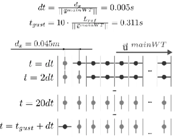
In order to make the side jet move along the main wind tunnel, the shutters are not all opened at once, but one by one, in sequence. The time between the opening of one door and the following is set up for having the “front” of the jet moving at the same speed of the main wind tunnel; the opening time of a single shutter corresponds instead to the desired wind gust duration. If this value is high enough to make the equivalent gust length greater than the width of the auxiliary wind tunnel (which is the case of the presented results), all the doors stay opened for the required duration, then close sequentially with
8 the same law (see Fig. 4).
Figure 4: Opening/closing door sequence scheme
2.2 TR-PIV measurements
Once the test bench was produced, the priority was to check if the generated gust could be considered realistic, that is if the transverse velocity seen at the future car model position had the expected stepwise evolution whereas the longitudinal component remained constant (Fig. 5).
Figure 5: Velocity vectors imposed by the two wind tunnels: (a) vector composition, (b) expected time evolution of the longitudinal and transverse component of velocity, at a generic point of the measurement zone
The main wind tunnel velocity was set to mainWT
u = 9 m/s, since this is the upper limit for the shutter system to operate the doors. The tests were held at atmospheric pressure and air temperature was 20°C.
The corresponding Reynolds number is Re u ref 1.68 105
mainWT
L
, based on the reference car
model length Lref = 0.28 m. The auxiliary wind tunnel velocity was set to uauxWT
= 9/cos(30°) = 10.39 m/s, in order to satisfy the vector relation shown in Fig. 5a with the imposed relative angle
9
between the wind tunnels. This gives a transverse velocity component of v = 5.20 m/s. The case of a wind gust duration of 10 vehicle lengths, corresponding to mainWT
ref gust L
t 10 u = 0.311 s, was studied.
An experimental campaign based on time resolved PIV was made to finely characterize the evolution of the side jet in the main steady flow. The results have to match the desired velocity profile (Fig. 5). We used a PIV system provided by Dantec: the laser is a Nd-YLF, with a lengthwave of 527 nm, energy 20 mJ per pulse and a maximal frequency of 10 kHz. A iNanoSense MkIII camera, with CCD sensor resolution of 1280 1024 pixels and maximal sampling frequency of 1 kHz, was also used. The flow was seeded upstream of each wind tunnel fan. Smoke generators were set up in order to guarantee an homogeneous smoke concentration in the measurement region. Moreover, the Stokes number (defined as the ratio of the response time of the seeded particle and the characteristic time of
the studied phenomenon,
ref ref s p sd L St u 18 2
, where ρs and µs are the density and the molecular viscosity
of the seeder and dp the particle diameter) was calculated from laser diffraction measurements. We had
St = 0.002, indicating that the chosen seeding particles will behave as good gas tracers.
PIV acquisitions were synchronized to first shutter opening, by means of a trigger signal generated by the driving interface of the test bench, so that phase averaging was possible. It was observed that the repeatability of the results is quite high, therefore all the presented results are averages of 15 runs. The sampling frequency was 500 Hz.
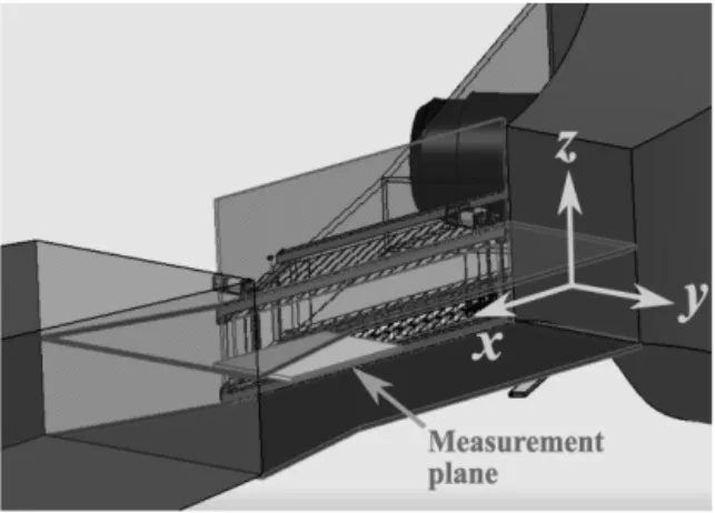
In Fig. 6 the measured field is represented: it is a horizontal plane located at half-height of the section of the main wind tunnel, corresponding to the 3/4 of height of the car model in its future position; this field was decomposed in 9 windows, each one sizing (134 105) mm2.
10
Figure 6: Part of geometry from Fig. 2 (enlarged side view) with position of the measurement plane
The velocity fields were calculated by means of the Dantec software “Flowmanager”, more precisely they were deducted from adaptive cross-correlation of images (see [23]): a 64 pixels final size of the interrogation area and a 50% overlap granted a spatial resolution of 3.5 mm.
The vectors were validated by means of two filters, based on signal to noise ratio and spatial velocity fluctuation.
3 Numerical approach
The used software is ICEM v11 for grid generation and Fluent v6.3 for solving fluid equations.
3.1 Continuous Navier-Stokes equations
The governing equations of the simulation are the well-known Unsteady Reynolds Averaged Navier-Stokes equations (URANS) of momentum and the equation of continuity restrained to incompressible flows. All the terms presenting a “+” symbol in the following averaged equations indicate their non-dimensional form. The physical quantities used as reference are the car body length Lref, the
longitudinal velocity of the main wind tunnel uref = umainWT and the air molecular viscosity . For a
generic point of coordinates (x+, y+, z+) at a generic time instant t+, the corresponding velocity vector will be expressed as u(u+,v+,w+) in the (x,y,z) reference defined in Fig. 6. Let us recall the URANS equations, in their dimensionless form with the Einsteinnotation:
11 0 u = x+j + j and + j + j + i t + i + + j i + j + + i x x Re + Re + x p = x u + t u 1 1 u u 2 (1) where t ref ref t ν L =
Re u . The Boussinesq turbulent kinematic viscosity νt is unknown in the URANS
approaches. The two chosen turbulence URANS models used in this work are Spalart-Allmaras [24] and SST k-ω [25].
In Spalart-Allmaras turbulence model the kinematic numerical viscosity is directly resolved by means of a single differential equation. A new parameter is introduced,
1 ν + t + f ν ν~ , representing a non-dimensional damped turbulent viscosity. The term
1 ν
f is a viscous damping function, whose formulation is detailed in [24].
Even if the readers can easily find the equation of Spalart [24], let us rewrite its equation in its dimensionless form and briefly show the meaning of each term:
term trip ~ of diffusion ~ of n dissipatio 2 ~ of production 2 ~ of transport u u Re ~ ~ ~ ~ 1 Re 1 ~ Re 1 ~ ~ Re 1 2 1 ~ u ~ 1 2 2 2 1 1 2 3 2 1 j j t j j b j j t b w w ij ij t b j j f x x C x x d f C f C d f f f C x t (2)
where the unknown is ν~ , + ij is the rotation tensor and
ref
L d
d is the non-dimensional distance to
the nearest wall. For further explanation of the other terms and constants, see [24; 26].
non-12 dimensional turbulent kinetic energy 2
' ' u u u 2 1 ref i i
k (where ui'ui' 2k, with k the turbulent kinetic
energy) and the non-dimensional specific dissipation rate
k L x x ref k i k i 09 . 0 u u' '
. These variables are
related to the dimensionless turbulent kinematic viscosity in equation (1) by the relation, + kω
+ + t f ω k = ν ,
where fkωis a damping function which has the same goal as fν1 in Spalart-Allmaras model. Each
quantity is resolved by a new dimensionless transport equation:
k j t k j k k j i ij k j j x k x k k x x k t k of diffusion of n dissipatio * of production * of transport Re 1 10 , u min u (3) term diffusion cross 1 of diffusion of n dissipatio 2 of production of transport 1 1 2 Re 1 2 u 2 1 j j j t j ij ij j j x x k F x x x t (4)
More information on the introduced terms can be found in [25; 26].
The partial differential equations (1-4) are discretized into a set of algebraic equations using the finite volume approach, which are then solved in an iterative fashion.
3.2 Computational grid and boundary conditions
The geometry of the numerical domain aims at reproducing the very same test bench presented in paragraph 2.1 and is represented in Fig. 7. The geometry of the auxiliary wind tunnel is faithfully
13
reproduced from the honeycomb straightener to its outlet in the main wind tunnel; the length and height of the main wind tunnel are the same as the real model. Its width is twice the wind tunnel section, to avoid numerical problems when placing a pressure outlet boundary condition too near to the studied region. The size of the domain is 7.05 5.7 1.34 non-dimensional lengths. A structured grid was set up, counting 1.4 million cells; the quality of 90% of elements, measured with the determinant method, is above 0.55 and the worst element quality is 0.32: the minimum recommended quality to avoid calculation errors is usually 0.2.
In Fig. 7, the mathematical formulations of inlets/outlets boundary conditions are also shown. At the inlets the velocity components are set to corresponding values in the real test bench (see paragraph 2.2). Turbulence boundary conditions are given by the hydraulic diameter
H L H L H L L L L D 2 (LL and LH being
the length and the height of the considered section, respectively) and turbulence intensity ratio
i i i i I u u u u' '
(where uiui is the mean velocity magnitude). The latter quantity was estimated by hot-wire
probe measurements and is I = 2% for both the main and auxiliary inlets.
Once these values are known, it is possible to set the turbulence values at each boundary. For Spalart – Allmaras simulation, the following formula was used [26]:
H i i + t D I = ν u u 0.07 2 3 (5)
For SST k-ω simulation, the values of k and + ω at the inlets were calculated with [26]: +
H ref + + ref i i + D L k = ω ; I = k 0.038 u u u 2 3 2 2 (6)
14
The corresponding value of the non dimensional Boussinesq turbulent kinematic viscosity ν+t can be calculated by means of the fkωfunction, previously presented.
The outlets of the fluid are simulated by setting to zero the pressure gauge between the static pressure on the face and the atmospheric pressure.
Figure 7: Three dimensional CFD: geometry and boundary conditions
The 20-channel shutter system was also reproduced (Fig. 8): the channel walls and the shutters have been simplified with simple planes. In particular, each shutter was designed both in its closed and opened position. The shutter actuation is simulated by setting a wall boundary condition (no velocity and zero normal pressure gradient) to the right plane, as explained in Fig. 8a. It is easy to reproduce with this approach the opened and closed shutter configurations, as shown in Fig. 8c, where the last five interior walls have been hidden to make the image clear.
Our approach is different than Ryan's 2D simulations [16]. As a matter of fact, his test bench is represented by a rectangle with no auxiliary wind tunnel. To replace it, transient Dirichlet boundary conditions on a side of the rectangle are imposed. The way the shutters are modeled is quite similar to ours. Indeed, the side representing the auxiliary wind tunnel presents 20 subsegments on which the inlet velocities are set respecting the opening shutter sequence represented in Fig. 4.
Returning to the discussion of our simulations, the technique described in this paper implies some simplification hypothesis: in first place, the shutters are supposed to open/close instantly (less than on
15
time step), when the actuation time is around 12 ms for opening and 30 ms for closing for the experimental test bench.
The shutter geometry was also simplified by ignoring its axis and by placing it orthogonally to the channel (Fig. 8b): this was made for having better element quality in the auxiliary wind tunnel. This simplification also implies that the closed shutters are perfectly airtight whereas some air leak is present on the real test bench. After the simulation, the value of the non dimensional CFD wall distance
c + CFD h y * u
(where u* is the friction velocity of the fluid and hc the distance of the barycenter of the
first computational cell from the wall boundary) was checked. It was seen that it varied from 51 to 89. According to FLUENT’s guide recommendations [25], both Spalart –Allmaras and SST k-ω model perform well if y+CFD >30.
Figure 8: Shutter system CFD simplification: (a) shutter boundary conditions, (b) comparison between real and simplified shutters, (c) example of the use of shutter boundary conditions.
A second order central difference scheme was used for space discretization, whereas time was discretized by means of an implicit first order scheme.
16
The solution was initialized with the results of a preliminary steady state simulation of the test bench with all the shutters in closed configuration. The time step size was constant and set to 2 ms.
4 Numerical and experimental results
The origin of the reference system, represented in Fig. 6, is placed at the beginning of the main wind tunnel in the center of the lower half section.
The u+ components of the steady state imposed velocity in both wind tunnels respect the condition
auxWT + mainWT
= u
u+ as shown in Fig. 5. The dimensionless time,
ref ref + L t =
t u represents the number of reference lengths covered by the main
flow.
We recall that, because of the setup of the PIV system, t+ = 0 corresponds to first shutter opening.
When t+ = 1, the main flow has covered one model length.
Even if the geometry of the system is three-dimensional, it has been observed that w+ << u+ in the measurement zone, so that it will only be discussed on u+ and v+ components of velocity.
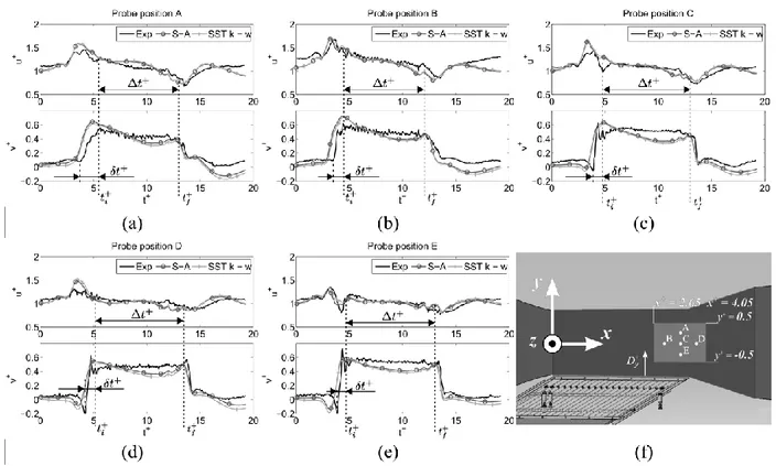
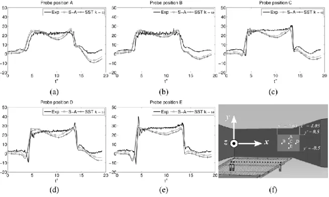
Figure 9 shows the evolution of u+ and v+ for five chosen points, both in terms of PIV measurements and CFD results. The coordinates of the chosen five points, as well as the non-dimensional distance
y
D to the end of the auxiliary wind tunnel, are reported in Tab. 1. It is easy to recognize in all the presented graphs the passage of the gust at the chosen points. In the following, we will identify with t+i the instant of the arrival of the gust front and with t+f the end of its passage (see Fig. 9a). In the time delay Δt between + ti+ and t+f , the considered point is subject to the fully developed flow coming from
the auxiliary wind tunnel. We will call this period the “established phase”.
17
imposed gust,t+gust=10, as shown in Fig. 4. The difference between Δt and + t+gust is partially due to the presence of a delay to reach the established phase. Let us note this delay δt+, as represented in Fig. 9a. It will be discussed on the δt+ value further. Moreover, there is also an additional delay after t+f when returning to the starting flow conditions.
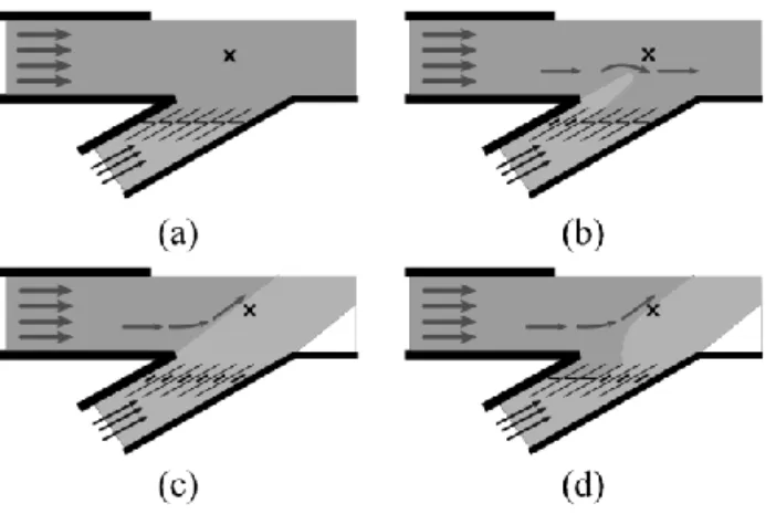
The evolution of u+ is different from the expected constant (see Fig. 6b), especially because of the overshoots at ti+ and t+f . Figure 10 provides a scheme explaining this phenomenon, already described
in [27]. In these drawings, the flows coming from each of the two wind tunnels are marked with a different color. At the start of the gust (Fig. 10b), the flow coming from the main wind tunnel is forced to bypass the jet front from the auxiliary wind tunnel. The main flow accelerates, giving the u+ velocity overshoot visible in Fig. 9. For +f
+ +
i <t <t
t , u+ gets its correct value (Fig. 10c) because the transverse flux has fully developed. When t+ t+f , the shutters are closing, so that the auxiliary air mass is progressively no more alimented by its wind tunnel (Fig. 10d). The main flow has to evacuate the residual air mass, the latter becoming a pressure drop for the former. The longitudinal velocity component of the main flow is then reduced, creating the u+ undershoot visible at t+f . These
imperfections are due to this kind of testbench: as a matter of fact, such profile was also seen in the hot-wire measurements by Ryan.
Concerning the component v+, its profile is similar to the desired evolution of a stepwise function (see Fig. 5b), except for the delay δt+. The value of δt+ increases with the distance to the shutter system, from 0.8 in position E to 1.5 in position A, corresponding to 24.9 and 46.7 ms, respectively. Nevertheless, these delays can be considered short enough to be approximated as instantaneous, when measuring unsteady forces.
18
velocity component v+. In particular, the nearest the point is to the end section of the auxiliary wind tunnel, the more these peaks are intense. Such a behavior was also seen by Ryan. The undershoot is caused by the main flow bypassing the auxiliary one (see again Fig. 10b). Concerning the overshoot, Ryan thought it could be due to the honeycomb straightener equipped on his test bench between the shutters and the end section of the auxiliary wind tunnel. In our test bench, this element is not present, but the imperfection still subsists. Another hypothesis could be the different pressure drop between the “opened” and “closed” shutter configuration (Fig. 3), generating undesired over-speeds in every channel of the shutter device when changing to “opened” configuration (for example in the scheme of Fig. 10b). This issue will be born in mind when setting the auxiliary wind tunnel velocity during the next campaign in presence of the car body.
If we focus on CFD results, it is possible to see that the dynamics is quite well reproduced, especially for u+ velocity. There is no particular difference of behavior for the two chosen turbulence models. The model fits well the experimental results, even if it tends to anticipate the arrival of the gust and reduce its velocity. It is also visible that the peak for v+ velocity fades too slowly and the established phase is not properly attained. The difference might come from the fact that the numerical actuation of the shutters is modeled by an instantaneous boundary condition switch, whereas the experimental sequence takes time, 12 ms for opening and 30 ms for closing, as illustrated in Fig. 8 from section 3.2. Because of the instantaneous opening of the numerical shutters, the differences on flow development as mentioned before (Fig. 10) between experiment and calculations are more visible during starting and finishing phases. Logically, crosswind penetration is also stronger in numerical approach than in experimental tests. The situation is reversed when the shutters are passing to the closed configuration (Fig. 10d), so that there is a kind of imbalance that causes slight oscillations in numerical values of v+. When planning this model, a way to avoid this phenomenon could have been the use of moving grid for
19
shutters, but it was discarded in order to keep the model as simple as possible and to avoid other problems such as those mentioned by Tsubokura et al. [17]. As explained in the introduction, even if some results could be processed by these authors, they presented important numerical irregularities caused by errors in calculation of the mass flow when the grid was changing.
Figure 9: Unsteady gust, profiles of non-dimensional velocity components in 5 points. Comparison of TR-PIV data with CFD models results. (a) to (e), profile at homonymous point, (f) chosen points and measuring field positions.
Probe position x+ y+ Dy A 3.75 0.35 1.15 B 3.25 0 0.8 C 3.75 0 0.8 D 4.25 0 0.8 E 3.75 -0.35 0.45
20
Figure 10: Scheme explaining the unsteady profile of longitudinal velocity u+ in test section. The “X” is marking the considered point. (a): Pure longitudinal flow, (b): Gust arrival, (c): Steady gust, (d): Gust passage.
Comparing the different results among the five positions, it appears that the best agreement between numerical and experimental results is achieved at point E, especially for u+ velocity. Nevertheless, the unsteady effects for v+ are very strong at this position, as for the experimental data. This is consistent with the fact that it is the nearest point to the shutters. At point E, the delay δt+ for the gust establishment is indeed the lowest, the velocity v+ is the highest during the established phase, and the velocity u+ keeps quite constant. This effect will be carefully taken into account when selecting the future position of a car body. Indeed, no confusion will have to be made between these overshoots due to the test bench facility and real dynamical unsteady efforts.
The numerical model was used to check if the presence of the shutter system affects the flow in the measurement region. A simulation of steady crosswind without the shutter system was then set up. We observed that the flow turbulence is only incremented in the auxiliary wind tunnel and in a small part of the main wind tunnel. For non dimensional distances Dy greater than 0.4 there is little difference among the two cases. Even, when Dy > 0.7, the turbulence of the case presented in Fig. 9 is lower than in the simulation without shutters. As an example, at point C, the turbulence intensity is 2.1% during the established phase (t+ = 7.97), and 2.5% in the simulation without the shutters. As a matter of fact,
21
the shutter system walls homogenize the flow exiting the auxiliary wind tunnel, as an honeycomb would do.
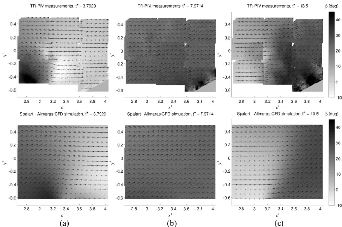
One important parameter for evaluating the quality of the reproduced gust is the yaw angle β. For a given point of the measurement region, at a time t+, it is defined as the angle between the velocity u
and the x direction: +
+ = x , = β u v arctan u .
Moreover, it is known (Baker [28]) that in steady yaw wind tunnel tests the most important efforts, such as side force and roll moment, proportionally increase with β. The yaw angle is expected to approach 30°, the angle between the two wind tunnels.
In Fig. 11, some snapshots of yaw angle field are represented: at the gust arrival (t+ = 3.79, Fig. 11a), during the established phase (t+ = 7.97, Fig. 11b) and at the passage of the gust (t+ = 13.82, Fig. 11c). Both turbulence models gave quite the same results, as seen in Fig. 9, so only Spalart Allmaras model is used for this comparison. A masked region is visible in the PIV results because of lack of seeding when measuring in these positions.
Even if some discrepancies are visible between TR-PIV measurements and numerical results, there is a good agreement, in Fig. 11b, when the gust is fully developed across all the test section, at t+ = 7.97. Then, at t+ = 13.82, for x+ > 3.2, the gust has nearly crossed the measurement region, as shown in Fig. 11c: this is well predicted by the CFD model. The main differences appear when simulating the arrival of the gust front: the CFD model is in little advance, comparing to experimental data.
22
Figure 11: Unsteady gust, TR-PIV measurements vs Spalart – Allmaras CFD simulations of yaw angle field. (a) : t+ =3.79, (b) : t+ =7.97, (c) : t+ =13.5
The evolution of β, for the same 5 positions of Fig. 9, is represented in Fig. 12. If yaw angles are compared to the respective velocity components evolutions (Fig. 9), it is possible to see that the effect of v+ dominates over u+, so that the imperfections of the latter will not be taken into account.
Concerning experimental results, the yaw angle obtained during the established phase tends to reach the imposed angle of 30° between the two wind tunnels, varying from 23° at position A to 27° at position E. Nonetheless, because of the greater influence of v+, the very same sequence of undershoot / overshoots appears for the points nearer to the end of the auxiliary wind tunnel. In particular, the overshoot at position E visible at t+ = 4.7 is 30% greater than the β value during the established phase. This fact has to be carefully considered when placing the model in the wind tunnel, since this percent is also the variation measured for aerodynamic actions in moving model tests ([4-7]).
23
In CFD results, yaw angle does not succeed to stabilize during the established phase, because of strong crosswind penetration, due to the instantaneous switches of boundary conditions, as previously explained. As the phenomenon described in Fig. 10 is accentuated, the overshoots and undershoots at
+ i
t and t+f , are more intense, so that a kind of imbalance makes the yaw angle slightly oscillate.
However, it qualitatively reproduces the experimental trends and can also predict the undershoot/overshoot sequence at +
i
t when approaching to the shutter system.
Figure 12: Unsteady gust, profiles of yaw angle β in 5 points. Comparison of TR-PIV data with CFD models results. (a) to (e), profile at homonymous point, (f) chosen points and measuring field positions.
The results presented in Figure 12 allowed us to define the best model position for the further campaigns. In ideal conditions, it would be better to work near to the end of the auxiliary wind tunnel, because of the greater yaw angle and of the smaller values of the delay δt+. However, the undershoot/overshoot values at +
i
t are important, relating to established values, and they can pollute the unsteady measurement of the aerodynamic effort. Therefore, we have planned to place the car model
24
further from the auxiliary wind tunnel end, in order to have a yaw angle evolution approaching to the ideal condition. In particular, we decided to put the windward flank of the vehicle so that it is aligned with points B, C, and D, see Tab. 1. The recommended position for the model geometrical center is (x = 3.43, y = 0.33).
5 Conclusions
A test bench reproducing the passing of a lateral unsteady gust on a vehicle, based on the double wind tunnel proposed by Ryan and Dominy [16], was built and validated by means of TR-PIV. This test bench, designed with a series of shutters at the end of an auxiliary wind tunnel, reproduces yaw angles decreasing with the distance to the shutters and spacing from 23 to 27°. These are typical values of high speed ground vehicles, who suffer relevantly from unsteady aerodynamic effects. The yaw angle is similar to the desired evolution of a stepwise function except for the presence of a delay to attempt the established phase. Even if it increases with the distance to the shutter system, it has been observed that it remained very short everywhere, compared to the gust duration.
During that nearly instantaneous time, an undershoot/overshoot sequence is visible just before the established phase of the gust, for positions near to the end of the auxiliary wind tunnel. The peak value of yaw angle reached during this sequence can be up to 30% greater than the one seen in the established phase. It has to be paid attention to this phenomenon because such kind of overshoots can be seen for aerodynamic efforts in moving model facilities. When writing this paper, a new experimental campaign is near to start. This time, a car model will be put in the test section and aerodynamic efforts will be measured with an unsteady balance. Thanks to the results presented here, it has been possible to state that it is safer to put the model far from the shutters in order to avoid the parasitical overshoots, even if the yaw angles are lower than the project value. If some effort peaks will
25
be seen, they will be representative of the true unsteady response of the vehicle, rather than being possible consequences of the yaw overshoots introduced by the test bench.
Meanwhile, a 3D CFD model based on URANS equations was developed and compared to these experimental results. It was possible to see that the flow dynamics is quite well reproduced, especially for the longitudinal velocity. The model fits well the experimental results, even if it tends to anticipate the arrival of the gust. As far as the yaw angle values are concerned, slight oscillations might come from the fact that the numerical actuation of the shutters is modeled by an instantaneous boundary condition switch, whereas the experimental sequence takes time, 12 ms for opening and 30 ms for closing. These sudden switches cause a kind of imbalance that does not allow the stabilization of yaw angle values during the expected established phase. When planning this model, a way to avoid this phenomenon could have been the use of moving grid for shutters, but it was discarded in order to keep the model as simple as possible and to avoid other problems such as those reported by Tsubokura et al. [17]. Better results can be achieved by discretizing the auxiliary wind tunnel outlet on a greater number of shutters whose width is smaller, but at this stage of research, we wanted to reproduce faithfully the same geometry of the ISAE test bench, and compare to the preliminary results. When writing this paper, a new numerical campaign was started, this time replacing completely the instantaneous boundary condition switch by the introduction of a concentrated pressure drop in the shutter region. The shutter actuation can now be simulated by a smooth change of the boundary conditions. The preliminary results are encouraging, since no oscillations of the transverse velocity component were seen.
References
[1] Hémon, P., and Noger C., 2004, “Transient Growth of Energy and Aeroelastic Stability of Ground Vehicles”, Comptes Rendus Mécanique 332, pp. 175–180.
26
[2] Baker, C. J., 1986, “A Simplified Analysis of Various Types of Wind Induced Road Vehicle Accidents”, Journal of Wind Engineering and Industrial Aerodynamics 22, pp. 69–85.
[3] Hucho, W. H., 1989, “Aerodynamics of Road Vehicles”, SAE International, pp. 214–234, Chap. 5. [4] Beauvais, F., 1967, “Transient Nature of Wind Gust Effects on an Automobile”, SAE Technical Paper 670608.
[5] Cairns, R. S., 1994, “Lateral Aerodynamic Characteristics of Motor Vehicles in Transient Crosswinds”, Ph. D. thesis, Cranfield University, U.K.
[6] C. J. Baker, and Humphreys, N. D., 1996, “Assessment of the Adequacy of Various Wind Tunnel Techniques to Obtain Aerodynamic Data for Ground Vehicles in Cross Winds”, Journal of Wind Engineering and Industrial Aerodynamics 60, pp. 49–68.
[7] Chadwick, A., 1999, “Crosswind Aerodynamics of Sports Utility Vehicles”, Ph. D. thesis, Cranfield University, U.K.
[8] Garry, K. P., and Cooper, K. R., 1986, “Comparison of Quasi-Static and Dynamic Wind Tunnel Measurements on Simplified Tractor-Trailer Models”, Journal of Wind Engineering and Industrial Aerodynamics 22, pp. 185–194.
[9] Chometon, F., Strzelecki, A., Ferrand, V., Dechipre, H., Dufour, P. C., Gohlke, M., and Herbert, V., 2005, “Experimental Study of Unsteady Wakes Behind an Oscillating Car Model”, SAE Technical paper 2005-01-0604.
[10] Cooper, R., 1984, “Atmospheric Turbulence with Respect to Moving Ground Vehicles”, Journal of Wind Engineering and Industrial Aerodynamics 17, pp. 215–238.
[11] Baker, C. J., 1991, “Ground Vehicles in High Cross Winds Part II: Unsteady Aerodynamic Forces”, Journal of Fluids and Structures 5, pp. 91–111.
27
to Evaluate the Aerodynamic Effects on Rail Vehicle Dynamics”, Vehicle System Dynamics 41, pp. 707–716.
[13] Bearman, P., and Mullarkey, S., 1994, “Aerodynamic Forces on Road Vehicles Due to Steady Side Winds and Gusts”, Proceedings of RAeS Conference on Vehicle Aerodynamics, Loughborough, U.K. [14] Passmore, M., Richardson, S., and Imam, A., 2001, “An Experimental Study of Unsteady Vehicle Aerodynamics”, Proceedings of Institution of Mechanical Engineers Part D–Journal of Automobile Engineering 215, pp. 779–788.
[15] Dominy, R., 1991, “A Technique for the Investigation of Transient Aerodynamic Forces on Road Vehicles in Cross Winds”, Proceedings of the Institution of Mechanical Engineers, Part D– Journal of Automobile Engineering 205, pp. 245–250.
[16] Ryan, A., 2000, “The Simulation of Transient Cross-Wind Gusts and Their Aerodynamic Influence on Passenger Cars”, Ph. D. thesis, University of Durham.
[17] Tsubokura, M., Kobayashi, T., Nakashima, T., Nouzawa, T., Nakamura, T., Zhang, H., Onishi, K., Oshima, N., 2009, “Computational Visualization of Unsteady Flow around Vehicles Using High Performance Computing”, Computers and Fluids 38, pp. 981–990.
[18] Tsubokura, M., Nakashima, T., Kitayama, M., Ikawa, Y., Doh, D. H., and Kobayashi, T., 2010, “Large Eddy Simulation on the Unsteady Aerodynamic Response of a Road Vehicle in Transient Crosswinds”, International Journal of Heat and Fluid Flow 31, pp. 1075–1086.
[19] Favre, T., 2011, “Aerodynamic Simulations of Ground Vehicles in Unsteady Crosswind”, Ph. D. Thesis, KTH School of Engineering Sciences, Stockholm, Sweden.
[20] Hemida, H., and Krajnovic, S., 2009, “Transient Simulation of the Aerodynamic Response of a Double-Deck Bus in Gusty Winds”, ASME Journal of Fluids Engineering 131.
28
of RAeS Conference on Vehicle Aerodynamics, Loughborough, UK.
[22] Macklin, A., Garry, K., and Howell, J., 1996, “Comparing Static and Dynamic Testing Techniques for the Crosswind Sensitivity of Road Vehicles”, SAE paper 960674, pp. 39–45.
[23] Dantec Dynamics GmbH, 2000, “FlowManager software and Introduction to PIV Instrumentation”, Publ. No.: 9040U3625.
[24] Spalart, P. R., and Allmaras, S. R., 1994, “A One-Equation Turbulence Model for Aerodynamic Flows”, La Recherche Aerospatiale, 1, pp. 5–21.
[25] Menter, F., 1994, “Two-equation Eddy-Viscosity turbulence Models for Engineering Applications”, AIAA Journal 32, pp. 1598–1605.
[26] Fluent Inc, 2006, “FLUENT User’s Guide”.
[27] Volpe, R., Ferrand, V., and Da Silva, A., 2011, “Validation d’un banc d’essais reproduisant les rafales de vent sur véhicule terrestre. Caractérisation de l’écoulement par TR-PIV”, Proceedings of 14ème congrès Français de Visualisation et de Traitement d’Images en Mécanique de Fluides – FLUVISU 14, Lille, France.
[28] Baker, C. J., 1991, “Ground Vehicles in High Cross Winds Part I: Steady Aerodynamic Forces”, Journal of Fluids and Structures 5, pp. 69–90.