HAL Id: tel-03112849
https://tel.archives-ouvertes.fr/tel-03112849
Submitted on 17 Jan 2021HAL is a multi-disciplinary open access
archive for the deposit and dissemination of sci-entific research documents, whether they are pub-lished or not. The documents may come from teaching and research institutions in France or abroad, or from public or private research centers.
L’archive ouverte pluridisciplinaire HAL, est destinée au dépôt et à la diffusion de documents scientifiques de niveau recherche, publiés ou non, émanant des établissements d’enseignement et de recherche français ou étrangers, des laboratoires publics ou privés.
Thibaut Montes
To cite this version:
Thibaut Montes. Numerical methods by optimal quantization in finance. Probability [math.PR]. Sorbonne University UPMC, 2020. English. �tel-03112849�
quantification optimale en finance
Numerical methods by optimal quantization in finance
Thibaut Montes
Laboratoire de Probabilités, Statistique et Modélisation - UMR 8001 Sorbonne Université
Thèse pour l’obtention du grade de :
Docteur de l’université Sorbonne Université
Sous la direction de : Gilles Pagès
Vincent Lemaire
Rapportée par : Giorgia Callegaro
Benoîte de Saporta
Présentée devant un jury composé de : Giorgia Callegaro (rapporteure)
Benoîte De Saporta (rapporteure) Jean-Michel Fayolle (invité) Benjamin Jourdain (président) Idris Kharroubi (examinateur)
Vincent Lemaire (co-directeur de thèse) Gilles Pagès (directeur de thèse)
Huyên Pham (examinateur) Abass Sagna (examinateur)
École Doctorale de Sciences Mathématiques de Paris-Centre
Tout d’abord, je souhaite exprimer ma gratitude envers mes directeurs de thèse Vincent Lemaire et Gilles Pagès qui m’ont accompagné tout au long de mon doctorat, m’ont fait confiance et ont toujours été disponibles pour répondre à mes questions. J’ai énormément appris à leurs côtés et leur en suis extrêmement reconnaissant. Leur supervision complémentaire est tout ce que je souhaite à leurs futurs doctorants. Elle m’a permis d’accomplir plus, à la fois en théorie et en pratique, que je n’aurais pu l’imaginer au début du doctorat. Je remercie également Jean-Michel Fayolle pour avoir rendu possible cette thèse CIFRE et de s’être investi pour rendre possible le dialogue entre ma recherche académique et les développements pratiques d’ICA.
Merci à mes deux rapporteures Giorgia Callegaro et Benoîte de Saporta d’avoir pris le temps de lire mon manuscrit de thèse. J’ai été très honoré de la confiance dont leurs rapports témoignent. Je tiens également à exprimer toute ma reconnaissance envers Benjamin Jourdain, Idris Kharroubi, Huyên Pham et Abass Sagna d’avoir accepté de faire partie de mon jury de thèse.
Je tiens également à remercier l’ensemble des doctorants que j’ai eu la chance de croiser durant ma thèse. On ne peut pas ne pas citer les thésards du bureau 201/3 (Léa, Rancy, Guillermo, Armand, Nicolas et Nicolas, Romain et Babacar) pour les cafés, les déjeuners en soum-soum au Restaurant du Personnel et les bières partagées. Je n’oublie pas non plus tous les autres doctorants que j’ai eu la chance de rencontrer et d’apprendre à connaitre durant les différentes conférences (le CEMRACS avec ses calanques - Métabief et son restaurant de raclette - Padoue et ses spritz). Je souhaite également remercier mes collègues chez ICA avec qui j’ai pu échanger, autour d’un café, d’un déjeuner ou d’un jogging, en particulier, Guillaume, Eric, Vincent, Emmanuel et Lauriane.
Je voudrais ensuite remercier ma famille, Jeanine ma maman, Amélie ma soeur, Joëlle ma marraine, mes oncles et tantes Michel et Elisabeth, Monique et Michel ainsi que mes cousines et cousins, pour avoir toujours cru en moi et avoir été présent, surtout dans les moments difficiles. Je tiens également à remercier Hélène, la maman de Julie, et toute la famille Besnard-Corblet-Hatzopoulos pour m’avoir soutenu et encouragé dès notre rencontre et encore plus durant ma thèse.
Je souhaiterais également remercier tous mes amis pour de merveilleux moments partagés et qui, par effet de bord, m’ont aidé à écrire cette thèse en rendant la vie plus douce. En particulier, je remercie Juju pour toutes ces années d’amitiés qui me sont précieuses ; Pierre,
Patrick et Cécile pour toutes ces soirées / week-ends gastronomalcooliques ; les Scubes et leur +1 (Grégory, Henrik et Anita, Howon, Laure, Léa, Julien et Christina, Anh-Mai, Thomas, Jérôme, Vincent et Gamze, Juliette) pour leur bonne humeur permanente ; Laurène et Robin pour ces longues et étranges heures passées à l’opéra ; Kevin et John pour leurs soirées à thème et pour finir Karine et Myriam pour ces très bonnes années à Aix-en-Provence.
Enfin et surtout, merci Pauline pour ton soutien inconditionnel et pour avoir toujours cru en moi. Tu m’as toujours poussé à aller plus loin, à prendre confiance en moi et ce depuis le début de notre rencontre. Merci pour avoir toujours pris le temps de m’écouter (même lorsque je radote "un peu").
This thesis is divided into four parts that can be read independently. In this manuscript, we make some contributions to the theoretical study and financial applications of optimal quantization.
In the first part, we recall the theoretical foundations of optimal quantization as well as the classical numerical methods to build optimal quantizers.
The second part focuses on the problem of numerical integration in dimension 1. This problem arises when one wishes to numerically compute expectations, such as the valuation of derivatives in finance that are expressed as the expectation of a function of a single financial asset. We recall the existing strong and weak error results and extend the results of order 2 convergence rate to other function classes with less regularity. In a second step, we present a weak error development result in one dimension and a second development in a higher dimension when the chosen quantizer is a product quantizer.
In the third part, we look at a first numerical application. We introduce a stationary Heston model in which the initial condition of volatility, instead of being deterministic as in the standard model, is assumed to be randomly distributed with the stationary distribution of the CIR EDS governing volatility. This variant of the original Heston model produces for European options on short maturities a steeper smile of implied volatility than the standard model. We then develop a product recursive quantization-based numerical method for the valuation of Bermudan options and barriers.
The fourth and last part deals with a second numerical application, the pricing of Bermudan exchange rate options in a 3 factor model, i.e. where the exchange rate, domestic and foreign interest rates are stochastic. These products are known in the markets as PRDC (Power Reverse Dual Currency). We propose two schemes to evaluate this type of options, both based on optimal product quantization and establish a priori error estimates.
Cette thèse est divisée en quatres parties pouvant être lues indépendamment. Dans ce manuscrit, nous apportons quelques contributions à l’étude théorique et aux applications en finance de la quantification optimale.
Dans la première partie, nous rappelons les fondements théoriques de la quantification optimale ainsi que les méthodes numériques classiques pour construire des quantifieurs optimaux.
La seconde partie se concentre sur le problème d’intégration numérique en dimension 1. Ce problème apparait lorsque l’on souhaite calculer numériquement des espérances, tel que l’évaluation de produits dérivés en finance qui s’expriment sous la forme d’un calcul d’espérance d’une fonction d’un unique actif financier. Nous y rappelons les résultats d’erreurs forts et faibles existants et étendons les résultats des convergences d’ordre 2 à d’autres classes de fonctions moins réguliers. Dans un deuxième temps, nous présentons un résultat de développement d’erreur faible en dimension 1 et un second développement en dimension supérieure pour un quantifieur produit.
Dans la troisième partie, nous nous intéressons à une première application numérique. Nous introduisons un modèle de Heston stationnaire dans lequel la condition initiale de la volatilité, au lieu d’être déterministe comme dans le modèle standard, est supposée aléatoire de loi la distribution stationnaire de l’EDS du CIR régissant la volatilité. Cette variante du modèle d’Heston original produit pour les options européennes sur les maturités courtes un
smile de volatilité implicite plus prononcé que le modèle standard. Nous développons ensuite
une méthode numérique à base de quantification récursive produit pour l’évaluation d’options bermudiennes et barrières.
La quatrième et dernière partie traite d’une deuxième application numérique, l’évaluation d’options bermudiennes sur taux de change dans un modèle 3 facteurs, i.e où le taux de change, les taux d’intérêts domestiques et étrangers sont stochastiques. Ces produits sont connus sur les marchés sous le noms de PRDC (Power Reverse Dual Currency). Nous proposons deux schémas pour évaluer ce type d’options toutes deux basées sur de la quantification optimale produit et établissons des estimations d’erreur à priori.
List of Figures xiii
List of Tables xvii
List of Algorithms xix
1 Introduction 1
1.1 Optimal Quantization . . . 1
1.1.1 Definitions and key findings . . . 1
1.1.2 Construction of an optimal quantizer . . . 4
1.2 Numerical integration . . . 8
1.2.1 Convergence rate of the weak error . . . 8
1.2.2 Weak error expansion of higher order . . . 10
1.2.3 Variance reduction . . . 12
1.3 Examples of applications in finance . . . 14
1.3.1 Stationary Heston Model . . . 14
1.3.2 Pricing of Bermudan options in a 3-factor model (PRDC) . . . 20
2 Introduction - Français 27 2.1 Quantification Optimale . . . 27
2.1.1 Définitions et principaux résultats . . . 27
2.1.2 Construction d’un quantifieur optimal . . . 30
2.2 Intégration numérique . . . 34
2.2.1 Convergence faible . . . 35
2.2.2 Développement d’erreur faible d’ordre supérieur . . . 37
2.2.3 Réduction de variance . . . 39
2.3 Exemples d’applications à la finance . . . 41
2.3.1 Modèle d’Heston Stationnaire . . . 41 2.3.2 Évaluation d’options bermudiennes dans un modèle 3 facteurs (PRDC) 47
3 Optimization of Optimal Quantizers 55
3.1 Theoretical foundations . . . 55
3.2 How to build an optimal quantizer? . . . 58
3.2.1 Real valued random variables: d “ 1 . . . . 58
3.2.2 Higher dimension: d ě 2 . . . . 71
Appendix 3.A Proof for the formulas of FX and KX . . . 80
4 New Weak Error bounds and expansions for Optimal Quantization 85 4.1 About optimal quantization (d “ 1) . . . . 90
4.2 Weak Error bounds for Optimal Quantization (d “ 1) . . . . 96
4.2.1 Piecewise affine functions . . . 96
4.2.2 Lipschitz Convex functions . . . 98
4.2.3 Differentiable functions . . . 102
4.3 Weak Error and Richardson-Romberg Extrapolation . . . 106
4.3.1 In dimension one . . . 107
4.3.2 A first extension in higher dimension . . . 108
4.4 Applications . . . 111
4.4.1 Quantized Control Variates in Monte Carlo simulations . . . 111
4.4.2 Numerical results . . . 114
5 Stationary Heston model: Calibration and Pricing of exotics using Product Recursive Quantization 125 5.1 The Heston Model . . . 127
5.2 Pricing of European Options and Calibration . . . 129
5.2.1 European options . . . 129
5.2.2 Calibration . . . 132
5.3 Toward the pricing of Exotic Options . . . 138
5.3.1 Discretization scheme of a stochastic volatility model . . . 138
5.3.2 Hybrid Product Recursive Quantization . . . 140
5.3.3 Backward algorithm for Bermudan and Barrier options . . . 150
5.3.4 Numerical illustrations . . . 153
Appendix 5.A Discretization scheme for the volatility preserving the positivity . . . 157
Appendix 5.B Lp-linear growth of the hybrid scheme . . . . 158
Appendix 5.C Proof of the L2-error estimation of Proposition5.3.4 . . . . 160
Appendix 5.D Quadratic Optimal Quantization: Generic Approach . . . 164
6 Quantization-based Bermudan option pricing in the F X world 169 6.1 Diffusion Models . . . 173
6.2 Bermudan options . . . 176
6.2.2 Backward Dynamic Programming Principle . . . 177
6.3 Bermudan pricing using Optimal Quantization . . . 182
6.3.1 About Optimal Quantization . . . 183
6.3.2 Quantization tree approximation: Markov case . . . 186
6.3.3 Quantization tree approximation: Non Markov case . . . 189
6.4 Numerical experiments . . . 195
6.4.1 European Option . . . 200
6.4.2 Bermudan option . . . 204
Appendix 6.A Wf is a Brownian motion under the domestic risk-neutral measure . 211 Appendix 6.B FX Derivatives - European Call . . . 212
1.1 Two quantizations of size N “ 100 of a centered Gaussian vector with identity covariance matrix. . . 3 1.2 Optimal Quantization of size N “ 11 of a standard Gaussian N p0, 1q. . . . 5 1.3 Two quantizations of size N “ 200 of a centered Gaussian vector with unit
covariance matrix. . . 6 1.4 Implicit volatility surface of the Euro Stoxx 50 on September 26, 2019. . . . 16 1.5 Implied volatility for 22 and 50 days maturity options after calibration without
penalty. . . 17 1.6 Implied volatility for maturity options 22 (left) and 50 (right) days after
calibra-tion with penalty. . . 18 1.7 Example of a PRDC payoff. . . 22 1.8 Pricing of Bermudan PRDC options yearly exercisable and maturing at 2, 5 or
10 years in a 3 factor model. . . 25 2.1 Deux quantifications de taille N “ 100 d’un vecteur gaussien centré et de matrice
de variance-covariance unitaire. . . 29 2.2 Quantification optimale de taille N “ 11 d’une gaussienne centrée réduite N p0, 1q. 31 2.3 Deux quantifications de taille N “ 200 d’un vecteur gaussien centré et de matrice
de variance-covariance unitaire. . . 32 2.4 Surface de volatilité implicite de l’Euro Stoxx 50 à la date du 26 Septembre
2019. . . 43 2.5 Volatilité implicite pour des options de maturité 22 et 50 jours après calibration
sans pénalisation. . . 44 2.6 Volatilité implicite pour des options de maturité 22 et 50 jours après calibration
avec pénalisation. . . 45 2.7 Exemple de payoff d’un PRDC. . . 50 2.8 Évaluation d’options PRDC bermudiennes exerçable annuellement et de maturité
2, 5 ou 10 ans dans un modèle 3 facteurs. . . 53 3.1 Two quantizations of size N “ 100 of a 2-dimensional standard Gaussian vector. 56
3.2 Optimal quantization of size N “ 11 of a standard normal distribution N p0, 1q. 59 3.3 Optimal quantization of size N “ 200 of pW1,suptPr0,1sWtq using the randomized
Lloyd method. . . 75 3.4 Example of division of a Voronoï cell CipΓNq into 5 triangles. . . 77
3.5 Two optimal quantizations of size N “ 100 and N “ 200 of a 2-dimensional standard Gaussian vector. . . 79 4.1 Pricing of a Call option in a Black-Scholes model with optimal quantization. . 116 4.2 Pricing of a Put-On-Call option in a Black-Scholes model with optimal quantization.118 4.3 Pricing of an Exchange spread option in a Black-Scholes model with optimal
quantization. . . 119 4.4 Pricing of an Exchange spread option in a Black-Scholes model with optimal
quantization (with Richardson-Romberg extrapolation). . . 120 4.5 Behavior in function of N of the pricing of a Basket option in a Black-Scholes
model with Monte Carlo using quantization-based control variates. . . 123 5.1 Implied volatility surface of the Euro Stoxx 50 as of the 26th of September 2019.132 5.2 Implied volatilities for 22 and 50 days expiry options after calibration without
penalization. . . 134 5.3 Implied volatilities for 7 and 14 days expiry options after calibration without
penalization. . . 134 5.4 Term-structure of the volatility in function of T and K of both Heston models
(stationary and standard) after calibration without penalization. . . 135 5.5 Relative error between market and models implied volatility after calibration
without penalization. . . 136 5.6 Implied volatilities for 22 and 50 days expiry options after calibration with
penalization. . . 137 5.7 Implied volatilities for 7 and 14 days expiry options after calibration with
penalization. . . 137 5.8 Relative error between market and models implied volatility after calibration
with penalization. . . 138 5.9 Example of recursive quantization of the volatility process in the Heston model
for one time-step. . . 141 5.10 Rescaled Recursive quantization of the boosted-volatility process with its
associ-ated weights from t “ 0 to t “ 60 days with a time step of 5 days with grids of size N “ 10. . . . 145 5.11 Prices of Bermudan options in the stationary Heston model given by product
5.12 Prices of Barrier options with strike K “ 100 in the stationary Heston model given by product hybrid recursive quantization. . . 156 6.1 Example of a PRDC payoff . . . 177 6.2 Domain of integration for probabilities of correlated two-dimensional Gaussian
random vector. . . 199 6.3 Relative errors for both methods based on product quantization for 2Y, 5Y and
10Y European options pricing (with zero correlations and σd“ σf “50bp). . . 202
6.4 Relative errors for both methods based on product quantization for 2Y, 5Y and 10Y European options pricing (with zero correlations and σd“ σf “500bp). . . 202
6.5 Relative errors for the non-Markovian method for 2Y, 5Y and 10Y European options pricing (with correlations). . . 204 6.6 Price with the two methods based on product quantization for 2Y, 5Y and 10Y
yearly exercisable Bermudan options (with zero correlations and σd“ σf “50bp).205
6.7 Relative differences between the two methods based on product quantization for 2Y, 5Y and 10Y yearly exercisable Bermudan options (with zero correlations and σd“ σf “50bp). . . . 206
6.8 Relative differences between the two methods based on product quantization for 2Y, 5Y and 10Y bi-annual exercisable Bermudan options (with zero correlations and σd“ σf “50bp). . . . 206
6.9 Price with the two methods based on product quantization for 2Y, 5Y and 10Y yearly exercisable Bermudan options (with zero correlations and σd“ σf “500bp).207
6.10 Relative differences between the two methods based on product quantization for 2Y, 5Y and 10Y yearly exercisable Bermudan options (with zero correlations and σd“ σf “500bp). . . . 207
6.11 Price of 2Y, 5Y and 10Y yearly exercisable Bermudan options using the non-Markovian method (with zero correlations and σd“ σf “50bp). . . . 209
3.1 Optimal quantization of the Gaussian distribution (with µ “ 0 and σ “ 1) using fixed-point search. . . 69 3.2 Optimal quantization of the Gaussian distribution (with µ “ 0 and σ “ 1) using
gradient descent. . . 70 3.3 Optimal quantization of the log-normal distribution (with µ “ 0 and σ “ 1). . . 71 3.4 Optimal quantization of the exponential distribution (with λ “ 1). . . . 71 4.1 Pricing of a Basket option in a Black-Scholes model with Monte Carlo using
quantization-based control variates. . . 122 5.1 Parameters obtained for both models after calibration without penalization. . . 135 5.2 Parameters obtained for both models after calibration with penalization. . . 136 5.3 Pricing of European options in a Stationary Heston model with product hybrid
recursive quantization with time-step n “ 180. . . . 154 5.4 Pricing of European options in a Stationary Heston model with product hybrid
recursive quantization with grids of size pN1, N2q “ p50, 10q. . . 155
6.1 Market values for the three factors model. . . 200 6.2 PRDC product description. . . 200 6.3 Prices given by closed-form formula of European options with zero correlations. 201 6.4 Computation times for European options pricing with zero correlations using
both methods based on product quantization. . . 203 6.5 Prices given by closed-form formula of European options with correlations. . . 203 6.6 Computation times for European options pricing with correlations using the
non-Markovian method. . . 204 6.7 Computation times for Bermudan yearly exercisable options pricing with zero
correlations using both methods based on product quantization. . . 208 6.8 Computation times for Bermudan yearly exercisable options pricing with
1 Lloyd method. . . 63
2 Anderson acceleration applied to Lloyd method. . . 65
3 Mean-field CLVQ. . . 66
4 Newton Raphson algorithm. . . 67
5 Newton Raphson algorithm with Levenberg-Marquart method. . . 68
6 Randomized Lloyd method. . . 73
Introduction
1.1
Optimal Quantization
This thesis is devoted to various theoretical aspects of optimal quantification in relation to numerical integration as well as several applications in finance. Optimal quantization was first introduced by Sheppard in 1897 in [She97]. His work focused on the optimal quantization of the uniform distribution over unit hypercubes. It was then extended to more general laws with or without compact support, motivated by applications to signal transmission in the Bell Laboratory in the 1950s (see [GG82]). Optimal quantization is also linked to an unsupervised learning computational statistical method. Indeed, the “k-means” method, which is a nonparametric automatic classification method consisting, given a set of points and an integer k, in dividing the points into k classes (“clusters”), is based on the same algorithm as the Lloyd method used to build an optimal quantizer. The “k-means” problem was formulated by Steinhaus in [Ste56] and then taken up a few years later by MacQueen in [Mac67]. In the 90s, optimal quantization was first used for numerical integration purposes for the approximation of expectations, see [Pag98], and later used for the approximation of conditional expectations: see [BPP01;BP03; BPP05] for optimal stopping problems applied to the pricing of American options, [PP05; PRS05] for non-linear filtering problems, [BDD13;PCR09;PPP04a;PPP04b] for stochastic control problems, [Gob+05] for discretization and simulation of Zakai and McKean-Vlasov equations and [BSD12; DD12] in the presence of piecewise deterministic Markov processes (PDMP).
1.1.1 Definitions and key findings
Let X be a random vector with values in Rdprovided with a |¨| norm, here always Euclidean, with
distribution PX, defined on a probability space pΩ, A, Pq such that X P L
2
Rd. The quantization
of X consists in approximating X by a random vector qpXq where q is a Borelian function with values in ΓN “ txN1 , . . . , xNNu ĂRd. In addition, we can see that distpX, qpXqq ě distpX, ΓNq
nearest neighbor projection ProjΓN is associated biunivocally with a Voronoï Borelian partition `CipΓNq ˘ 1ďiďN of R d such that CipΓNq Ă␣ξ P R, |ξ ´ xNi | ďmin j‰i |ξ ´ x N j |(.
Thus, the associated nearest neighbor projection is defined by
ProjΓNpξq “
N
ÿ
i“1
xNi 1ξPCipΓNq.
Such quantization is called “Voronoï ”. We will note pXΓN the closest neighbor projection of X
on ΓN “ txN1 , . . . , xNNu, then
p
XΓN “Proj
ΓNpXq.
We lighten the notation from pXΓN to pXN for clarity.
Then, the law of a quantizer pXN is entirely characterized by the centroid grid ΓN “
txNi ,1 ď i ď Nu in which the quantizer takes its values and the N-tuple of the weights pNi
which represent the probability that pXN is equal to xNi or, equivalently, that X belongs to the
Voronoï cell i, i.e.
pNi “P`XpN “ xNi
˘
“P`X P CipΓNq˘, i “1, . . . , N.
In this thesis, we’ll be working primarily with optimal quadratic quantization. The term
optimal comes from the fact that we look for the best approximation of X in the sense that we
will want to minimize the distance between the random vectors X and pXN by optimizing the
grid ΓN for a given size N. This distance is measured in L2-norm, hence the term quadratic.
The distance between X and pXN, denoted as }X ´ pXN}2, is called the mean quantization error.
But we often reason in terms of distortion which is none other than the square of the mean quantization error. For a N-tuple, it is defined by
Q2,N: x “ pxN1 , . . . , xNNq ÞÝÑE ” min i“1,...,N|X ´ x N i |2 ı “ }X ´ pXN}22.
So, we’re looking for the grid ΓN with cardinal at most N such that the quantifier pXN “
ProjΓNpXqminimizes
min
ΓNĂRd,|ΓN|ďN
}X ´ pXN}22.
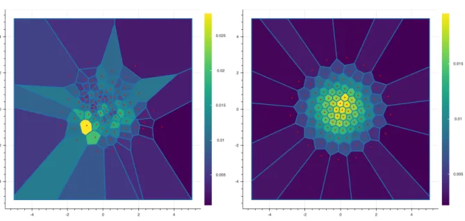
Such a grid always exists when X P L2 (see Theorem1.1.1below). In the Figure1.1, we present
two quantizations of size N “ 100 of a centered Gaussian vector with identity covariance matrix. On the left, we represent an i.i.d. sample of the Gaussian vector and on the right an optimal quantizer. The color of each cell represents the probability pN
i associated to the cell CipΓNq of
centroid xN
Fig. 1.1 Two quantizations of size N “ 100 of a centered Gaussian vector with identity covariance
matrix.
The minimization problem being set, several results have been demonstrated in the literature, see for example the two books [GL00; Pag18] for more details on the theory of optimal quantization. Let us note that this theory can be fully developed in a Lp framework and we
then speak of Lp-optimal quantization. We first mention a result that ensures the existence of
an optimal quantizer.
Theorem 1.1.1. (Existence of an optimal N-quantization) Let X P L2
RdpPq and N P N ‹.
(a) The quadratic distortion function Q2,N at the N level reaches a minimum in (at least)
one N-tuplet x‹ “ pxN
1 , . . . , xNNq and the associated grid Γ‹N “ txNi , i “1, . . . , Nu is called
an optimal N-quantizer.
(b) If the PX distribution support of X has at least N elements, then x
‹
“ pxN1 , . . . , xNNq
has pairwise distinct components and PX`CipΓ
‹
Nq
˘
ą 0, i “ 1, . . . , N. In addition, the
sequence N ÞÑ infxPpRd
qNQ2,Npxq converges to 0 and is strictly decreasing as long as it is
strictly positive.
In addition to knowing that the quadratic distortion decreases towards 0, the exact speed of convergence has been established through the contributions of several authors: [Zad82; BW82;GL00]. The theorem has been demonstrated in the Lp case and thus characterizes the
quantization error Lp.
Theorem 1.1.2. (Zador’s Theorem) Let d P N‹ and p P p0, `8q.
(a) Sharp rate. Let X P Lp`δ
Rd pPq with δ ą 0. Let PXpdξq “ φpξq ¨ λdpdξq ` νpdξq, where
a constant rJp,d P p0, `8q such that lim N Ñ`8N 1{d min ΓNĂRd,|ΓN|ďN }X ´ pXN}p “ rJp,d „ ż Rdφ d d`pdλ d ȷ1 p` 1 d
where pXN is an Lp-optimal quantization of X.
(b) Non-asymptotic upper-bound [GL00; Pag18]. Let δ ą 0. There exists a real
constant Cd,p,δP p0, `8q such that, for all random vector X with values in Rd,
@N ě1, min
ΓNĂRd,|ΓN|ďN
}X ´ pXN}p ď Cd,p,δσδ`ppXqN
´1{d
where, for r P p0, `8q, σrpXq “minaPRd}X ´ a}r ă `8.
1.1.2 Construction of an optimal quantizer
There are many methods to build an optimal quantizer. In some very rare cases, centroids are given explicitly, for example when X „ Upra, bsq where a, b P R, the ΓN grid is given by
ΓN “␣xN1 , . . . , xNN ( “ " 2i ´ 1 2N : i “ 1, . . . , N * .
We also refer to [GL00] for Laplace law and [FP02] for semi-closed formulas for exponential law, power law and inverse power law. However, most of the time this is not the case so we have to use iterative methods to construct the grids and weights associated with each of the centroids. These iterative methods are divided into two large families: deterministic methods (Lloyd’s algorithm, Newton-Raphson’s algorithm and their variants, ...) which are based on explicit knowledge of the density and the distribution function of the X law and methods based on stochastic optimization (Competitive Learning Vector Quantization (CLVQ), randomized version of the Lloyd’s algorithm, ...) requiring only the ability to simulate X. These methods are detailed in the Chapter3.
Case of a real-valued random variable - d “ 1. In the unidimensional case, we have
a result of uniqueness of the optimal quantizer when the density of X is log-concave. This theorem has been demonstrated by Kieffer in his [Kie82] (see also [Pag98]).
If X is a random variable (d “ 1) for which we know the first partial moment KXp¨qand
the cumulative distribution function FX of X
KXpxq:“ ErX 1Xďxs and FXpxq:“ PpX ď xq,
then we use in priority deterministic methods which allow to build very quickly an optimal quantizer of X, such as the Lloyd’s algorithm introduced in [Llo82] which is a fixed point
search algorithm. It is also possible to apply the Newton-Raphson algorithm by computing the Hessian of the quadratic distortion function (see [PP03] for a detailed example applied to a normal random variable). Other deterministic gradient descents can be used such as Levenberg-Marquardt or quasi-Newton methods. Otherwise, stochastic optimization-based methods such as the stochastic version of the Lloyd’s algorithm or a stochastic gradient descent are used (see [Pag98]).
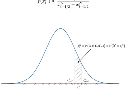
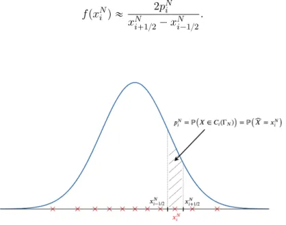
Example 1.1.3. In Figure 1.2, we represent in blue the density of a one-dimensional Gaussian
random variable and in red the centroids of the optimal quantizer of size N “ 11 of this same random variable. We also illustrate what the weights pN
i associated to the centroids xNi
represent. Moreover, we can approach the density (if it exists) at each point of the grid by the following relation
f pxNi q « 2p
N i
xNi`1{2´ xNi´1{2.
Fig. 1.2 Density of a reduced centered Gaussian N p0, 1q in blue and centroids of an optimal
quantizer size N “ 11 in red.
Case of a random vector - d ě2. Now, let us consider a X random vector with values in
Rd(d ě 2). Two approaches exist to construct an optimal quantizer of the law of X.
The first approach is to apply the methodology developed in the scalar case directly to the vector case and thus obtain an optimal quantification of X. If we know the density of X then it is still possible in dimension 2 or 3 to apply the deterministic methods (cf. Chapter 3). However, from d ě 4, we can only rely on stochastic optimization methods based on the simulation of samples of the X distribution.
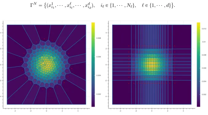
The second, product quantization, consists in constructing an optimal quantizer of each of the components of the random vector and then constructing the quantizer by considering the cartesian product between all the optimally quantized components. More precisely, that is
quantifiers pXℓ of size Nℓ of each of the marginal Xℓ. Each quantizer pXℓ takes its values from
the grid ΓNℓ
ℓ “␣ziℓℓ, iℓ P t1, ¨ ¨ ¨ , Nℓu
(
. Thus, the quantizer product of X takes its values in the grid ΓN which is the Cartesian product of the one-dimensional grids, i.e. ΓN “śd
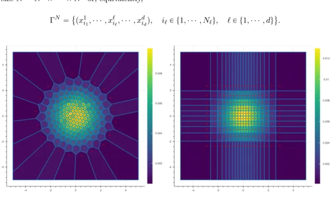
ℓ“1Γ Nℓ ℓ of size N “ N1 ˆ ¨ ¨ ¨ ˆ Nd or, equivalently, ΓN “␣px1i1, ¨ ¨ ¨ , x ℓ iℓ, ¨ ¨ ¨ , x d idq, iℓP t1, ¨ ¨ ¨ , Nℓu, ℓ P t1, ¨ ¨ ¨ , du(.
Fig. 1.3 Two quantizations of size N “ 200 of a centered Gaussian vector with unit covariance
matrix. Optimal quantization on the left and Product quantization on the right.
In the Figure1.3, we compare the optimal quantization and the product quantization of a centered Gaussian vector with unit covariance matrix. Both methods have their advantages and disadvantages, the first method produces a better quantization of the random vector X compared to the product quantization but the induced numerical cost for the construction of an optimal quantizer is often much higher.
Case of diffusions. If now, instead of considering a random vector, we are interested in
diffusions, i.e.
dXt“ bpt, Xtqdt ` σpt, WtqdWt
then there are, again, several solutions to quantize Xt. Specifically, given a time discretization
at n-step ptkq0ďkďn, we are looking for the quantisers pXtNkk of size Nk of Xtk that we denote
p
XNk
k and Xk in order to lighten the notations. The object we’re trying to construct is called a
quantization tree. A tree is characterized by the knowledge of the laws `Γk, ppkiq1ďiďNk
˘ of the
quantizers p pXkq0ďkďn and of the transition probabilities pki,j.
P`Xpk`1“ xk`1j | pXk“ xki˘.
We will not present all the existing approaches that allow us to address the problem of quantization of diffusion but only those that allow us to use deterministic numerical methods for the optimization of the grids. For other approaches, based on stochastic algorithms we refer to the series of papers [BPP01;BP03].
Quantization of marginal laws. The problem of quantization of a diffusion has been
initiated and developed in a series of articles [PPP04b;BPP05; BBP09; BBP10; CFG19]. If Xk
can be simulated exactly, that is without the help of a time discretization scheme, and that we know the marginal law of Xk, at each instant tk, then we are brought back to the case of the
quantization of a random vector. Indeed, we can optimally quantize each random vector Xk
using deterministic numerical methods if d ď 2, producing an optimal quantization tree, or we can optimally quantize each of its components and then construct a product quantization of
Xk, producing a product quantization tree.
Example 1.1.4. If we consider a Black-Scholes model with constant volatility σ and constant
interest rates r
dSt“ Stprdt ` σdWtq, avec S0 “ s0,
then we have an explicit form for St
St“ S0epr´σ
2{2qt`σW
t
so for a given date t, logpSt{S0q „ N
`
pr ´ σ2{2qt, σ2t˘ so we can optimally quantize Stat each
instant that interests us using deterministic methods (cf. Chapter3). We can also quantize the Brownian Wt which is “more universal”.
Recursive quantization. In the case where we do not know by the marginal law of
Xk and that we need to use a discretization scheme (Euler-Maruyama, Milstein, ...), we will
use a method called recursive quantization. Recursive quantization (also called Markovian quantization) was first introduced in [PPP04b] and then studied in depth in [PS15] for the case of a one-dimensional diffusion discretized by an Euler-Maruyama scheme. A fast algorithm based on deterministic methods to build the quantization tree is developed and analyzed. Subsequently, fast recursive quantization was extended to higher order one-dimensional schemes by [McW+18] and to higher dimensions by product quantization (see [PS18b; FSP18; Rud+17; CFG18; CFG17]). This method consists in building recursively in k the quantizers pXNk
k via the recursion p XNk k “ProjΓNk ` r Xk ˘ avec rXk“ Ek´1 ` p XNk´1 k´1 , Zk ˘
where Ek´1 is a discretization scheme.
1.2
Numerical integration
A common problem in practice is to calculate the expectation of a function of X when X is a variable or a random vector, i.e. E “fpXq‰. However, except in very particular cases, it is not possible to calculate explicitly this quantity, it is the case for example if X “ XT the value
of a diffusion at the date T . This is why it is necessary to use numerical integration methods. [Pag98] introduces a cubature method based on optimal quantization in order to approximate expectations of the form E “fpXq‰. Let us consider pXN an optimal quantizer of X, the fact
that pXN is discrete allows us to easily define the following cubature formula
E“fp pXNq‰“
N
ÿ
i“1
pNi f pxNi q. (1.1)
Furthermore, given that pXN was constructed as the best discrete approximation of X of
cardinal at most N then it seems reasonable to think that E “fp pXNq‰is a good approximation of E “fpXq‰.
In the Chapter4, taken from the article “New Weak Error bounds and expansions for Optimal Quantization” published in Journal of Computational and Applied Mathematics, see [LMP19], we present new results in the real case concerning the error induced by the quantization-based approximation of expectation E “fpXq‰. This is a joint work with Vincent Lemaire and Gilles Pagès and it is accessible inarXiv orHAL. These “weak” results are summarized below.
1.2.1 Convergence rate of the weak error
In the first part of Chapter4, we are interested in the rate of convergence from E “fp pXNq‰to E“fpXq‰ as a function of N for different classes of functions f when X is a random variable with values in R, i.e we look for the largest α ą 0 such that, for any function f in this class F,
lim N N αˇ ˇE“fpXq‰ ´ E “fp pXNq ‰ˇ ˇď Cf,Xă `8.
If we naively upper-bound the weak error by the strong error along the Lipschitz continuous functions, we obtain the following upper-bound (with α “ 1) for a sequence of N-quanifiers
L2-optimal N-quantifiers NˇˇE“fpXq‰ ´ E “fp pXNq ‰ˇ ˇď N rf sLip}X ´ pXN}1 ď N rf sLip}X ´ pXN}2 N Ñ`8 ÝÝÝÝÝÑ Cf ă `8
where Zador’s Theorem (1.1.2) was used. Moreover, if we consider fpxq “ distpx, ΓNq then f is
a Lipschitz continuous function and we have
NˇˇE“fpXq‰ ´ E “fp pXNq ‰ˇ
ˇ“ N }X ´ pXN}1 ď N }X ´ pXN}2 ÝN Ñ`8ÝÝÝÝÑ Cf ă `8.
For some classes of functions we can prove that the cubature formula induces a weak error of order 2 (α “ 2). For example, if we consider functions that are derivable with a Lipschitz continuous derivative then we have an error of order 2, see [Pag98]. Indeed, we use a Taylor expansion with an integral remainder of the form
f pxq “ f pyq ` f1 pyqpx ´ yq ` ż1 0 `f1ptx ` p1 ´ tqyq ´ f1 pyq˘px ´ yqdt and the stationarity property of an optimal quadratic quantizer as follows
E“X | pXN‰“ pXN.
The first term in the Taylor expansion is zero because
E“f1p pXNqpX ´ pXNq‰“E ” f1p pXNqE“X ´ pXN | pXN‰ ı “E ” f1p pXNq` E “X | pXN‰´ pXN˘ ı “0. Thus, using Lipschitz’s property of the derivative and Zador’s theorem, we get a weak error of order 2, as expected. N2ˇˇE“fpXq‰ ´ E “fp pXNq ‰ˇ ˇď N2 ż1 0 E“ˇˇf1ptX ` p1 ´ tq pXNq ´ f1p pXNq ˇ ˇ|X ´ pXN|‰dt ď rf 1s Lip 2 N2}X ´ pXN}22 N Ñ`8 ÝÝÝÝÝÑ Cf ă `8.
In the first part of Chapter4, we extend these results concerning the convergence rate of the weak error of order higher than 1 to a wider class of functions with less regularity, more precisely, functions that are either :
‚ Lipschitz continuous piecewise affine functions with finitely many breaks of affinity, ‚ Lipschitz continuous convex functions,
‚ differentiable functions with piecewise-defined locally Lipschitz derivative (K breaks of affinity ta1, . . . , aKu, such that ´8 “ a0ă a1 ă ¨ ¨ ¨ ă aKă aK`1“ `8 and the locally
Lipschitz property of the derivative is defined by
@k “0, . . . , K, @x, y P pak, ak`1q |f1pxq ´ f1pyq| ď rf1sk,Lip,loc|x ´ y|`gkpxq ` gkpyq
˘ where gk: pak, ak`1q ÑR` are non-negative Borel functions,
‚ differentiable functions with piecewise-defined locally α-Hölder derivative (K breaks of affinity ta1, . . . , aKu, such that ´8 “ a0ă a1 ă ¨ ¨ ¨ ă aKă aK`1“ `8 and the locally α-Hölder property of the derivative is defined by
@k “0, . . . , K, @x, y P pak, ak`1q, |f1pxq ´ f1pyq| ď rf1sk,α,loc|x ´ y|
α`g
kpxq ` gkpyq
˘ where gk: pak, ak`1q ÑR` are non-negative Borel functions,
For the first three classes of functions, we show that the weak error is of order 2 and for the last one, of order 1 ` α.
In the numerical part, we illustrate this result by evaluating the price of a European Call in a Black-Scholes model given by
I0 :“ E “ e´rTpST ´ Kq`
‰ where St “ S0epr´σ
2{2qt`σW
t with pW
tqtPr0,T s a Brownian motion. In order to approximate,
with the help of quantization, the price of the European Call we can rewrite I0 in two different
ways
I0“E“φpSTq
‰
“E“fpWTq
‰
where φ is a piecewise affine function with one affinity break and f is a differentiable function with a piecewise locally Lipschitz continuous derivative. Thus, when considering quantizers of
ST or WT and using the cubature formula, we observe, for both approximations, a weak error
of order 2.
1.2.2 Weak error expansion of higher order
In the second part of Chapter4, we are interested by the weak error expansion of the approxi-mation of E “fpXq‰ by E “fp pXNq‰
. That is, we’re looking expansion of the form
E“fpXq‰ “ E “fp pXNq‰` c2
N2 ` OpN ´p2`βq
q
where β P p0, 1s. In the previous section, we have already shown that the optimal quantization-based cubature formula approximation induces an error term of order OpN´2
qin the best case. Here, we seek to refine the previous results in order to obtain a “controlled” error expansion of order 2 and not a simple convergence rate of order 2.
In Section 4.3, we show that this expansion exists if the function f : R Ñ R is twice differentiable with a Lipschtiz continuous second derivative. This result uses a Taylor expansion of order 2 with an integral remainder of the form
f pxq “ f pyq ` f1pyqpx ´ yq ` 1 2f2pyqpx ´ yq2` ż1 0 p1 ´ tq`f2ptx ` p1 ´ tqyq ´ f2 pyq˘px ´ yq2dt
where we take the expectation on both sides of the equality and replace x and y with X and p
XN, respectively. The second term on the righthand side is cancelled using the stationarity
property of the optimal quadratic quantizer. For the third term, we rely on [Del+04] (Theorem 6) which states that @g : R Ñ R such that E “gpXq‰ ă `8
lim N N 2 E“gp pXNq|X ´ pXN|2‰“ Q2pPXq ż gpξq PXpdξq
that we apply to g “ f2 where Q
2pPXq is the Zador’s constant. Thus, we already have the first
two terms in the expansion of the error. For the last term, we use the Lipschitz property of the second derivative and the rest of the proof is based mainly on a result initially established in [GLP08] and then recently extended in [PS18a], known as “Lr-Ls distortion mismatch”,
which is formulated as follows : what can be said about the convergence rate of E “|X ´ pXN|s‰ knowing that pXN is a Lr-optimal quantizer when s ą r and X P Ls? We cite this theorem for d “1, which is the case we’re interested in.
Theorem 1.2.1 (Lr-Ls-distorsion mismatch). Let X : pΩ, A, Pq Ñ R a random variable and
r P p0, `8q. Let PXpdξq “ φpξq ¨ λpdξq ` νpdξq, where ν K λ i.e. ν is singular with respect
to the Lebesgue measure λ on R and φ is not identically null. Let pΓNqN ě1 a sequence of
Lr-optimal quantization grids and s P pr, r ` 1q. If
X P L1`r´ss `δpPq
for a δ ą0, so
lim sup
N
N }X ´ pXN}s ă `8.
So, applying this theorem with r “ 2 and s “ 2 ` β, we get a OpN´p2`βq
q for the last term and @ β P p0, 1q, we have the following expansion
E“fpXq‰ “ E “fp pXNq‰` c2
N2 ` OpN ´p2`βq
q.
This error expansion allows us to theoretically justify the use of Richardson-Romberg extrapolation which aims to kill the first error term of the expansion by linearly combining two quantification cubature formulas, respectively at N and M points, i.e.
E“fpXq‰ “ E « M2f p pXMq ´ N2f p pXNq M2´ N2 ff ` OpN´p2`βqq for M “ kN with k ą 1.
We illustrate this result in the numerical part by valuing a European spread option in a 2-dimensional Black-Scholes model whose price is given by
I0 :“ E “ e´rTpST1 ´ ST2 ´ Kq`‰.
By preconditioning, we express I0 as follows
I0“E“φpZ2q
‰
where Z2 is a standard Gaussian and φ is a twice differentiable function with a Lipschitz second
derivative. Thus, considering N-optimal quantizers pZN of Z2 „ N p0, 1q, we approximate I0
using the cubature formula based on optimal quantization (1.1) and observe a weak error of the order of 2. Moreover, using Richardson-Romberg extrapolation, we reach a weak error of the order of 3.
However, the relevance of the cubature method by optimal quantization when d “ 1 remains limited because it is in competition with methods based on Gauss points. A multi-dimensional extension is on the other hand very useful as soon as d “3. We consider a function twice differentiable f : Rd
ÞÑ R with a bounded and Lipschitz continuous Hessian. Furthermore, we assume that X : pΩ, A, Pq Ñ Rd has independent components X
k, k “1, . . . , d and that
the quantizer pXN is a product quantizer of X with d components p pXNk
k qk“1,...,d such that N1ˆ ¨ ¨ ¨ ˆ Nd“ N. So, we have E“fpXq‰ “ E “fp pXNq‰` d ÿ k“1 ck N2 k ` O ˆ ´ min k“1:dNk ¯´p2`βq˙ . 1.2.3 Variance reduction
In the last part of the Chapter4, we present a new variance reduction method of a Monte Carlo estimator with control variates based on one-dimensional optimal quantization. Other variance reduction methods based on optimal quantization have been developed, see for example [CP15; Pag18] for more details. This approach is motivated by the rate of convergence of order 2 of the weak error induced by the quantization-based cubature formula for various classes of functions, including those mentioned above.
The problematic. Let pZkqk“1,...,d“ Z P L2RdpPq a random vector and a function f : RdÑ
R. We’re interested in the following quantity
I :“ E “fpZq‰. (1.2)
Often we cannot compute this quantity explicitly, so a standard approach is to use a Monte Carlo estimator sIM :“ M1
řM
I. The convergence of the method and its rate are determined by the strong law of large
numbers and the central limit theorem, respectively, which ensure, if Z is of integrable square, that s IM p.s. ÝÝÑE“fpZq‰ and ?M ´ s IM ´E“fpZq‰ ¯ L ÝÑ N`0, σ2f pZq˘ when M Ñ `8 where σ2
f pZq“Var`fpZq˘. We notice that, for a given simulation size M, the limiting factor of
the method is σ2
f pXq, so variance reduction methods were developed in order to reduce the value
of σ2
f pXqand accelerate the convergence of the Monte Carlo estimator to I. The reader can refer
to [Pag18;Gla13] for more details on Monte Carlo simulation and variance reduction methods in general such as control variates, antithetic method, stratification, importance sampling, ...
A new method of variance reduction by quantized control variable. Let ΞN be a
random vector with values in Rd defined by
ΞN :“ pΞN
kqk“1,...,d,
which will be our d-dimensional control variable, each ΞN
k component is given by
ΞN
k :“ fkpZkq ´E“fkp pZkNq‰,
where fkpzq:“ fpErZ1s, . . . ,ErZk´1s, z,ErZk`1s, . . . ,ErZdsqand pZkN is an optimal quantization
of size N of Zk. We use here a unidimensional optimal quantization in order to take advantage
of the weak error results previously shown, indeed the functions fk : R Ñ R are part of the
classes of functions allowing us to reach a weak error of order 2. We introduce Iλ,N as an
approximation for (1.2) Iλ,N “E“fpZq ´ xλ,ΞNy‰“E « f pZq ´ d ÿ k“1 λkfkpZkq ff ` d ÿ k“1 λkE“fkp pZkNq ‰ (1.3)
where λ P Rd. The terms E “f kp pZkNq
‰
in (1.3) can be easily and quickly computed using the discreteness of quantizers.
At this point, we can define pIλ,N
M the Monte Carlo estimator associated to I
λ,N p IMλ,N “ 1 M M ÿ m“1 ˜ f pZmq ´ d ÿ k“1 λkfkpZkmq ¸ ` d ÿ k“1 λkE“fkp pZkNq‰.
It is important to notice that we introduce a bias when using such control variates, indeed for every k P t1, . . . , nu, ErΞN
ks ‰ 0 because E “fkp pZkNq
‰
is an approximation of E “fkpZkq
‰ . However, the quantity that really interests us is not the bias induced by the estimator pIλ,N
rather the Mean Squared Error (MSE) giving us a bias-variance decomposition MSEppIλ,N M q “ ˜ d ÿ k“1 λk ´ E“fkp pZkNq ‰ ´E“fkpZkq ‰¯ ¸2 looooooooooooooooooooooooomooooooooooooooooooooooooon biais2 ` 1 M Var ˜ f pZq ´ d ÿ k“1 λkfkpZkq ¸ loooooooooooooooooomoooooooooooooooooon
Variance du Monte Carlo .
Thus, we can take higher values of N to make the bias term negligible compared to the variance of the estimator while controlling the total cost induced by the Monte Carlo estimator. In practice, we do not need to take very high values for N. Indeed, the bias term converges to 0 as N´4 if f belongs to the right class of functions, so taking optimal quantifiers of size 200 is
more than enough to make the bias negligible compared to the variance of the Monte Carlo estimator. We develop this point in the third part of the Chapter4.
In the numerical part of the Chapter 4, we apply the variance reduction method to the valuation of a basket option in a Black-Scholes model in dimension d. The control variate allows us to divide the variance of the Monte Carlo estimator by 100 for small dimensions (d “ 2 or
d “3) and by 6 for larger dimensions (d “ 10). We also observe that the bias induced by the
quantification becomes negligible for grids with a size greater than 100 (N ą 100).
1.3
Examples of applications in finance
1.3.1 Stationary Heston Model
In Chapter 5, we are interested in the stationary Heston model and more precisely in the evaluation of European, Bermuda and barrier options in this model as well as the calibration of the model. Chapter 5corresponds to the preprint “Stationary Heston model: Calibration and Pricing of exotics using Product Recursive Quantization” accessible inarXivor HAL(see [LMP20]). This article is a joint work with Vincent Lemaire and Gilles Pagès.
The standard Heston model was originally introduced by Heston in [Hes93]. It is a stochastic volatility model where the initial volatility condition is assumed deterministic. This model has become very popular mainly for the following two reasons: it is a stochastic volatility model so it introduces a smile in the surface of the implied volatility as observed in the market and the characteristic function of this model is given by a semi closed-form formula which allows us to value European options (Call & Put) almost instantaneously (see Carr & Madan in [CM99]). However, a remark often made about this model is that the smile of implied volatility is not steep enough for short maturities compared to what is observed in the market (see [Gat11]). Noticing that the volatility process is ergodic with a single invariant distribution
ν “Γpα, βq where the α and β parameters depend on the volatility diffusion parameters, it
has been proposed by Pagès & Panloup in [PP09] to directly consider that the process evolves under its stationary regime instead of starting it at time 0 from a deterministic value. This
choice has the effect of accentuating the volatility smile for short maturities while keeping the same behavior as the standard model for longer maturities. Later, the short and long-term behavior of the implied volatility generated by such a model was studied by Jacquier & Shi in [JS17].
Thus, the diffusion of the asset-volatility couple pSpνq
t , vνtq in the stationary Heston model is
defined by $ ’ ’ & ’ ’ % dStpνq Stpνq “ pr ´ qqdt ` a vtν`ρdĂWt`a1 ´ ρ2dWt ˘ dvtν “ κpθ ´ vtνqdt ` ξ a vtνdĂWt where vν 0 „ Lpνq „Γpα, βq with β “ 2κ{ξ2, α “ θβ.
Valuation of European Options. First of all, in the first part of the Chapter5, we recall
the method used for the valuation of a Call in the standard Heston model. Starting from the knowledge of the characteristic function ψ`λpvq, u, T ˘ of the logarithm of the asset at date T (see [SST04;Gat11;Alb+07] for a robust choice of formula), the price of the Call of strike K
and maturity T on the asset Spvq
T in the standard Heston model where the volatility has as
initial condition v P R is given by
Cpϕpvq, K, T q “ E“e´rTpSTpvq´ Kq`
‰
“ s0e´qTP1`λpvq, K, T ˘ ´ Ke´rT P2`λpvq, K, T ˘
where the quantities P1`λpvq, K, T ˘and P2`λpvq, K, T ˘ are defined by
P1`λpvq, K, T ˘ “ 12 ` 1 π ż`8 0 Re ˆ e´iu logpKq iu ψ`λpvq, u ´ i, T ˘ s0epr´qqT ˙ du P2`λpvq, K, T ˘ “ 12 ` 1 π ż`8 0 Re ˆ e´iu logpKq iu ψ`λpvq, u, T ˘ ˙ du
with i the base of imaginary numbers (such that i2 “ ´1).
From this formula, we derive a method to compute the price I0 of a Call in the stationary
Heston model. Indeed, by preconditioning by vν
0, we have I0 “E “ e´rTφpSpνq T q ‰ “E“Cpϕpvν0q, K, T q‰.
Thus, in order to obtain an approximation of I0, we propose two methods. The first, based
on optimal quantization, consists in building an optimal quantizer of the gamma law Γpα, βq and then to use the cubature formula studied in the Chapter4. The second method is to use a quadrature formula based on Laguerre polynomials.
Calibration. Once we are able to price European options in the stationary Heston model,
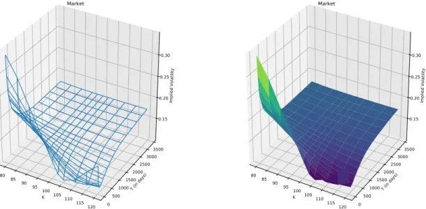
We also calibrate the standard Heston model to compare its implied volatility surface to the one of the stationary model. Both models are calibrated on the implied volatility surface of the Euro Stoxx 50 (see Figure1.4). Since we are interested in the short-term behaviour of the implied volatility surface, the calibration of the models is performed on options with a maturity of 50 days (T “ 50{365). We then observe the implied volatilities generated by the models for short-term maturities. K 80 85 90 95 100 105 110 115120 T (in d ays) 0500 10001500 20002500 30003500 Im plied Vo lat ility 0.15 0.20 0.25 0.30 Market K 80 85 90 95 100 105 110 115120 T (in d ays) 0500 10001500 20002500 30003500 Im pli ed Volat ilit y 0.15 0.20 0.25 0.30 Market
Fig. 1.4 Implicit volatility area of the Euro Stoxx 50 on September 26, 2019. (S0 “3541,
r “ ´0.0032 and q “ 0.00225)
The set of 4 parameters of the stationary Heston model to be calibrated is defined by
PSH “␣pθ, κ, ξ, ρq PR`ˆR`ˆR`ˆr´1, 1s(
and the 5 standard model parameters PH by
PH “␣px, θ, κ, ξ, ρq PR`ˆR`ˆR`ˆR`ˆr´1, 1s(.
The other parameters are directly observed in the market.
We can notice that the stationary model has one less parameter to be calibrated compared to the standard model, which makes its calibration more robust than the standard model which is known to be over-parameterized (see [guarantee2009fitting]). In practice, we observe that the calibration of the standard model is very dependent on the set of parameters used to initialize the optimization algorithm whereas it is not the case for the stationary model.
For the calibration of the models, the standard method consists in solving the following optimization problem min ϕPP ÿ K ˆ σM arket iv pK, T q ´ σ M odel iv pϕ, K, T q σM arket iv pK, T q ˙2
where the quantities σM arket
iv pK, T qand σ
M odel
iv pϕ, K, T qare, respectively, market implied
volatil-ities and those calculated with a Heston model of parameter ϕ “ pθ, κ, ξ, ρq or ϕ “ px, θ, κ, ξ, ρq in appropriate cases.
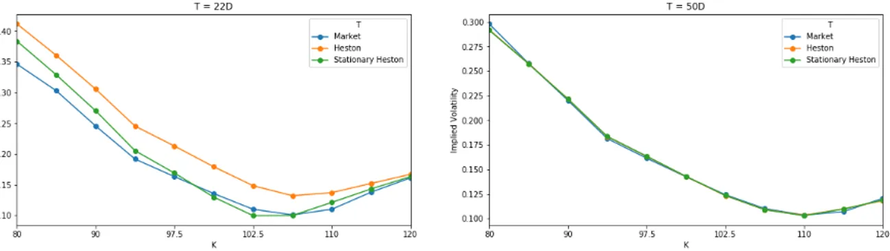
Fig. 1.5 Implied volatility for maturity options 22 (left) and 50 (right) days after calibration
without penalty.
In Figure1.5, we compare the implied volatility curves generated by the two models after calibration to European options with 50-day maturity. We observe that the stationary model produces a smile of volatility that is steeper than the standard model for options with a 22-day maturity. However, when we perform the calibration, we notice that the parameters obtained do not satisfy the Feller’s condition
ξ2 ď2κθ
which ensures the strict positivity of volatility. This property is important for the numerical valuation of exotic options discussed in the last part of the chapter.
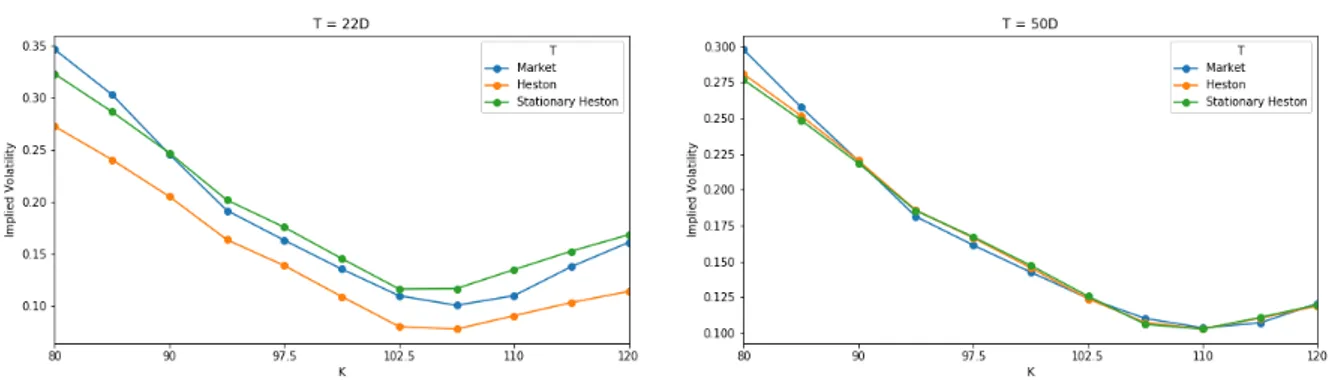
Thus, to obtain parameters that satisfy the Feller condition, we constrain the parameters by adding a penalty to the minimization problem that becomes
min ϕPP ÿ K ˆ σM arket iv pK, T q ´ σ M odel iv pϕ, K, T q σM arket iv pK, T q ˙2 ` λmaxpξ2´2κθ, 0q where λ is the penalty factor adjusted during the procedure.
Fig. 1.6 Implied volatility for maturity options 22 (left) and 50 (right) days after calibration
with penalty.
In the Figure 1.6, we make the same comparison as before. We notice that the addition of the penalty deteriorated the quality of the calibration at maturity 50 days. As for maturity 22 days, we observe that the stationary model again succeeds in producing a smile of volatility closer to that of the market than the standard model.
Exotic Options Valuation by Recursive Product Quantification. In the last part of
the Chapter5, we address the pricing of exotic options such as Bermudan options and barrier options using a Backward Dynamic Principle Programming. The numerical method we propose is based on recursive product quantization. We extend the methodology previously developed by [FSP18; CFG18; CFG17] where a Euler-Maruyama scheme was considered for the discretization in time of both assets and volatility.
Time discretization of diffusions. We made the choice to consider a hybrid scheme
composed of an Euler-Maruyama scheme for the dynamics of the log-active Xt“logpStpνqqand
a Milstein scheme for the boosted volatility process Yt“eκtvνt. Thus, we have
# s Xtk`1 “ Eb,σ`tk, sXtk, sYtk, Z 1 k`1 ˘ s Ytk`1 “ Mrb,rσ`tk, sYtk, Z 2 k`1 ˘
with tk “ kn, n the number of discretization time steps, Zk`11 „ N p0, 1q and Zk`12 „ N p0, 1q
such that CorrpZ1
k`1, Zk`12 q “ ρ. The Euler-Maruyama scheme is defined by
Eb,σpt, x, y, zq “ x ` bpt, x, yqh ` σpt, x, yq ? h z with bpt, x, yq “ r ´ q ´ e ´κty 2 and σpt, x, yq “e´κt{2 ? y,
and the Milstein schema put into its canonical form M rb,rσpt, x, zq “ x ´ r σpt, xq 2rσ1 xpt, xq ` h ˆ rbpt, xq ´pr σσr 1 xqpt, xq 2 ˙ `prσrσ 1 xqpt, xqh 2 ˆ z `? 1 hσr 1 xpt, xq ˙2 with rbpt, xq “eκtκθ, r σpt, xq “ ξ?xeκt{2 and rσ 1 xpt, xq “ ξeκt{2 2?x .
Product Markovian Recursive Quantization. Once the choice of the discretization
scheme in time has been made, we are interested in the discretization in space of the asset-volatility couple.
To do this, we first construct a Markovian quantization tree ppYtkqk“0,...,n. It is advantageous
to notice that the volatility is autonomous and therefore we face a one-dimensional problem. Thus, the quantizers pYtk are recursively constructed, i.e. pYtk`1 is an optimal quantizer of rYtk`1
defined by r Ytk`1 “ Mrb,σr`tk, pYtk, Z 2 k`1˘, Ypt k`1 “ProjΓY N2,k`1 ` r Ytk`1˘.
Numerically, we use the methods based on deterministic algorithms for the 1 dimension developed in Chapter3.
Now, using the fact that Ythas already been quantized, we construct a Markov quantization
tree p pXtkqk“0,...,n of Xt. Again we are brought back to a one-dimensional problem and we
construct the quantizers pXtk recursively, i.e. pXtk`1 is an optimal quantizer of rXtk`1 defined by
r Xtk`1 “ Eb,σ`tk, pXtk, pYtk, Z 1 k`1˘, Xpt k`1 “ProjΓX N1,k`1 ` r Xtk`1˘.
In order to alleviate the notations, we shall denote pXk and pYk instead of pXtk and pYtk.
Now that we have calibrated the stationary Heston model and are able to construct a quantization tree for the asset-volatility couple, we are interested in the evaluation of exotic options and more specifically Bermudan or barrier options.
Bermudan options. The price on date tk of a Bermudan option exercisable on dates
ttk, ¨ ¨ ¨ , tnu with payoff ψtkpXtk, Ytkq on the date tk is given by the Snell envelope Vk
Vk“ sup τ PTn k E ” e´rτψ τpXτ, Yτq | Ftk ı , where Tn
k represents the set of stopping times τ taking values in ttk, t1, . . . , tnu. The Backward
Dynamic Principle Programming allows to rewrite Vk as follows
#
Vn“e´rtnψnpXn, Ynq,
We then apply the methodology employed by [BP03; BPP05; Pag18] which consists in replacing Xkand Ykby the quantizers pXkand pYk. By construction of the recursive quantization,
the couple p pXk, pYkq is Markovian so we obtain the following Quantized Backward Dynamic Principle Programming # p Vn“ ψnp pXn, pYnq, p Vk “max `ψkp pXk, pYkq,Er pVk`1| p pXk, pYkqs˘, k “0, . . . , n ´ 1.
Finally, the price of the Bermudan option is given by E “pV0
‰ .
Barrier Options. The price on date tk of a barrier option with maturity T , payoff f and
barrier L is given by
PU O“e´rT E“fpXTq1suptPr0,T sXtďL‰.
For the valuation of the barrier option, we apply the algorithm based on the conditional law of Euler’s scheme, see [Gla13;Sag10;Pag18]. Thus, once the asset-volatility couple is discretized in time, the price PU O is rewritten as follows
s PU O“e´rT E“fp sXTq1suptPr0,T sXstďL ‰ “e´rT E „ f p sXTq n´1 ź k“0 Gkp sX k, sYkq, sXk`1pLq ȷ where Gkpx,yq,zpuq “ ´ 1 ´ e´2npx´uqpz´uqT σ2ptk,x,yq ¯ 1tuěmaxpx,zqu.
Finally, replacing sXk and sYk by pXk and pYk and using a recursive algorithm to approach
s PU O by ErpV0s, we have $ & % p Vn“e´rT f p pXnq, p Vk“E“Gkp pX k, pYkq, pXk`1pLq pVk`1 | p pXk, pYkq‰, 0 ď k ď n ´ 1.
1.3.2 Pricing of Bermudan options in a 3-factor model (PRDC)
In the Chapter 6, we address the problem of Bermudan exchange rate option pricing where stochastic domestic and foreign interest rates are considered. In this case, we refer to a three-factor model. Chapter 6 corresponds to the article “Quantization-based Bermudan option pricing in the F X world” submitted to Journal of Computational Finance and accessible in arXivorHAL (see [Fay+19]). This article is a joint work with Jean-Michel Fayolle, Vincent Lemaire and Gilles Pagès.
The need to evaluate such products originated in Japan at the end of the 20th century. Indeed, the persistence of low interest rates during the last decades of the century was one of the main reasons that led to the creation of exchange rate structured financial products. These