Elastic and elasto-dynamic models of robot manipulators

Handle ID: .http://hdl.handle.net/10985/9081

To cite this version :

Alexandr KLIMCHIK, Anatol PASHKEVICH - Elastic and elasto-dynamic models of robot manipulators - 2012

Any correspondence concerning this service should be sent to the repository Administrator : archiveouverte@ensam.eu

Projet COROUSSO

ANR‐10‐SEGI‐003

Tâche 1 :

Conception Optimale et Modelisation

du Robot Porteur

Livrable 1.1 :

Modèles élastiques et élasto‐dynamiques

de robots porteurs

Projet ANR‐2010‐SEGI‐003‐COROUSSO

Partenaires :

Liste de diffusion

Nom Organisme Fonction

ANR

Rédigé par Approuvé par Validé par

Date 24/02/2012 24/02/2012 15/05/2013

Nom(s) _{A. PASHKEVITCH} A. KLIMCHIK A. PASHKEVITCH G. ABBA

Signature(s)

Indice de

révision Modifié par Description des principales évolutions Date de mise en application concernées Pages

Auteurs : AK, AP

S

S

O

O

M

M

M

M

A

A

I

I

R

R

E

E

1

Introduction ... 5

2

Robot-based processing of high-performance materials ... 8

2.1

Modern trends in machining ... 8

2.2

Machining of high performance materials ... 10

2.3

Machining with robots versus traditional machining tools ... 14

2.4

References ... 22

3

Stiffness matrix of robotic manipulators with passive joints ... 25

3.1

Introduction ... 25

3.2

Motivation example ... 27

3.3

Passive joints in a serial chain ... 29

3.4

Passive joints in a parallel manipulator ... 31

3.5

Computational techniques ... 32

3.5.1

Recursive computations: single-joint decomposition ... 32

3.5.2

Analytical computations: chains with trivial passive joints ... 33

3.6

Application examples ... 37

3.7

Conclusion ... 40

3.8

Appendix A : Properties of stiffness matrix K

C

... 40

3.9

Appendix B: Recursive computation of the stiffness matrix K

C

... 42

3.10

References ... 43

4

Stiffness modeling of robotic-manipulators under auxiliary loadings ... 46

4.1

Introduction ... 46

4.2

Problem statement ... 47

4.3

Static equilibrium equations ... 48

4.4

Static equilibrium configuration ... 49

4.5

Stiffness matrix ... 50

4.6

Illustrative examples ... 53

4.6.1

Serial chain with torsional springs ... 53

4.6.2

Serial chains with torsional and translational springs ... 55

4.7

Conclusion ... 56

4.8

References ... 57

5

Stability of manipulator configuration under external loading ... 59

5.1

Introduction ... 59

5.2

Problem statement ... 60

5.2.1

Motivation ... 60

5.2.2

Basic assumptions and research problems ... 62

5.3

Stability of kinematic chain configuration under loading ... 62

5.3.1

Static equilibrium ... 62

5.3.2

Stability criterion ... 64

Auteurs : AK, AP

5.4

Stability of The end-platform location under external loading ... 65

5.4.1

Cartesian stiffness matrix of a serial kinematic chain ... 66

5.4.2

Cartesian stiffness matrix of parallel manipulator ... 66

5.5

Application examples ... 68

5.5.1

Stiffness analysis for serial chain with 1D-springs ... 68

5.5.2

Stability of serial chain under auxiliary loading ... 71

5.5.3

Kinetostatic singularity in the neighborhood of the flat configuration ... 73

5.6

Conclusions... 75

5.7

References ... 75

6

Stiffness modeling of non-perfect parallel manipulators ... 77

6.1

Introduction ... 77

6.2

Stiffness modeling background ... 78

6.3

Stiffness models aggregation for small loading ... 79

6.3.1

Stiffness model aggregation for perfect chains ... 79

6.3.2

Stiffness model aggregation for non-perfect chains ... 80

6.4

Stiffness models aggregation for high loading ... 82

6.4.1

Stiffness model of parallel manipulator ... 82

6.4.2

Compliance model of parallel manipulator ... 85

6.5

Application examples ... 86

6.5.1

Aggregation non-perfect serial chains without loading ... 86

6.5.2

Aggregation non-perfect serial chains under loading ... 88

6.6

Conclusion ... 89

6.7

References ... 90

7

Compliance error compensation technique for parallel robots composed of non-perfect

serial chains ... 92

7.1

Introduction ... 92

7.2

Problem of compliance error compensation ... 93

7.3

Stiffness modeling background ... 96

7.4

Nonlinear technique for compliance error compensation ... 97

7.5

Illustrative example: compliance error compensation for milling ... 100

7.6

Conclusions... 104

7.7

References ... 105

8

Conclusions ... 107

Auteurs : AK, AP

1 INTRODUCTION

At present, aerospace and ship building industries progressively replace conventional materials by new ones that provide essential advantages from the point of view of mechanical properties of the final products, but at the same time introduce some complexity in the manufacturing process. In particular, machining of modern high‐performance materials requires revision of some approaches in design and programming of manufacturing cells that must provide high accuracy and high productivity simultaneously.

In machining of such materials, currently there are two main trends. The first of these is based on conventional CNC‐machines that are provided by dedicated cutting tools, which are able to achieve desired quality and productivity. However, this classical approach has essential limitations and can be hardly applied when a workpiece geometry is complicated and its dimensions are rather large. In this case, the second trend, which is based on industrial robotic manipulators, looks very attractive. This type of machining cells can be implemented using either serial or parallel manipulators. Both approaches have their advantages and disadvantages. In particular, serial robots provide large workspace but usually are quite heavy and the influence of gravity forces is significant. In contrast, in parallel manipulators the gravity influence is essentially smaller (but not negligible), while the work envelop is limited by particularities of this architecture. Aside these, in both cases the cutting forces produce essential compliance errors that influence the quality of the final product. For this reason, stiffness analysis of robotic manipulators under essential external forces becomes a critical issue in design of robotic‐based manufacturing cells for machining of modern high‐ performance materials.

In literature, the main results in manipulator stiffness analysis are obtained assuming that the compliance errors are small enough and may be evaluated by linear models. However, for the considered application area this assumption should be revised, which requires development of relevant non‐linear stiffness modeling techniques that are able to evaluate the compliance errors caused by different types of external and internal loadings (cutting and gravity forces, internal preloading in joints introduced in order to eliminate backlash, forces generated by gravity compensators, internal stresses caused by assembling of non‐ perfect over‐constrained closed‐loops in parallel manipulators, etc.). Another difficulty is related to taking into account the influence of passive joints that are numerous in parallel manipulators. Hence, the manipulator stiffness modeling for these industry‐motivated conditions is a challenge in robotic science.

In this work, to develop the desired stiffness model and corresponding compliance error compensation technique, the Virtual Joint Modeling (VJM) concept is used. This choice is motivated by its essential advantages for the considered application areas, such as high computational efficiency and acceptable accuracy. Compared to other alternative approaches (Finite Element Analysis, Matrix Structural Analysis), the VJM technique is more suitable for both on‐line and off‐line modes, but it should be essentially enhanced to ensure stiffness modeling in the cases of significant external/internal forces for manipulators with passive joints. In addition, the models to be developed should be able to detect some certain non‐linear effects in the stiffness behavior of the manipulator under high loading (buckling for instance). In addition, existing approaches implicitly assume that all robot components are perfect and there are no internal stresses caused by assembling of over‐constrained structure. So, in spite of the fact that the problem of stiffness modeling of serial and parallel manipulators was in the focus of numerous researches, the main results are in the area of linear stiffness analysis and there are still a number of open theoretical questions, some of which will be considered in this report.

Auteurs : AK, AP

This report focuses on enhancement of stiffness modeling techniques for serial and parallel manipulators in order to increase the accuracy and efficiency of robotic‐based machining of high performance materials by means of compensation of the compliance errors (in on‐line or/and off‐line mode). To achieve this goal, several problems have to be solved:

Problem 1:

Enhancement of VJM‐based stiffness modeling technique for serial and parallel manipulators with arbitrary location of passive joints in the case of small deflections (unloaded mode).

Problem 2:

Extension of the proposed VJM‐based technique for the case of large deflections caused by internal and external loadings, taking into account related changes in Jacobians and equilibrium coordinates.

To address the above defined problems, the thesis is organized as follows:

Chapter 2 is devoted to the state of art and literature review on the robotic based processing of high performance materials. It includes a review of robot applications for machining of high performance materials, determination of potential demands, limitations and advantages.

Chapter 3 focuses on stiffness matrix computation for manipulators with passive joints, compliant actuators and flexible links. It proposes both explicit analytical expressions and an efficient recursive procedure that are applicable in general case and allow obtaining the desired matrix either in analytical or numerical form. Advantages of the developed technique and its ability to produce both singular and non‐ singular stiffness matrices are illustrated by application examples that deal with stiffness modeling of two Stewart‐Gough platforms.

Chapter 4 focuses on the extension of the virtual‐joint‐based stiffness modeling technique for the case of different types of loadings applied both to the robot end‐effector and to manipulator intermediate points (auxiliary loading). It is assumed that the manipulator can be presented as a set of compliant links separated by passive or active joints. It proposes a computationally efficient procedure that is able to obtain a non‐linear force‐deflection relation taking into account the internal and external loadings. It also produces the Cartesian stiffness matrix. This allows to extend the classical stiffness mapping equation for the case of manipulators with auxiliary loading. The results are illustrated by numerical examples.

Chapter 5 is devoted to the analysis of robotic manipulator behavior under internal and external loadings. The main contributions are in the area of stability analysis of manipulator configurations corresponding to the loaded static equilibrium. In contrast to other works, in addition to usually studied the end‐platform behavior with respect to the disturbance forces, the problem of configuration stability for each kinematic chain is considered. The proposed approach extends the classical notion of the stability for the static equilibrium configuration that is completely defined the properties of the Cartesian stiffness matrix only. The advantages and practical significance of the proposed approach are illustrated by several examples that deal with serial kinematic chains and parallel manipulators. It is shown that under the loading the manipulator workspace may include some specific points that are referred to as elastostatic singularities where the chain configurations become unstable.

Auteurs : AK, AP

chains, whose geometrical parameters differ from the nominal ones. In these manipulators, there usually exist essential internal forces/torques that considerably affect the stiffness properties and also change end‐effector location. These internal loadings are caused by elastic deformations of the manipulator elements during assembling, while the geometrical errors in the chains are compensated by applying appropriate forces. For this type of manipulators, a non‐linear stiffness modeling technique is proposed that allows us to take into account inaccuracy in the chains and to aggregate their stiffness models for the case of both small and large deflections. Advantages of the developed technique and its ability to compute the compliance errors caused by different factors are illustrated by an example that deals with parallel manipulator of the Orthoglide family.

Chapter 7 presents the compliance errors compensation technique for over‐constrained parallel manipulators under external and internal loadings. This technique is based on the non‐linear stiffness modeling which is able to take into account influence of non‐perfect geometry of serial chains caused by manufacturing errors. Within the developed technique, the deviation compensation reduces to a proper adjusting of a target trajectory that is modified in the off‐line mode. The advantages and practical significance of the proposed technique are illustrated by an example that deals with groove milling with Orthoglide manipulator that considers different locations of the workpiece. It is also demonstrated that the impact of the compliance errors and the errors caused by inaccuracy in serial chains cannot be taken into account using the superposition principle.

Finally, Chapter 8 summarise the main contribution of this report

Auteurs : AK, AP

2 ROBOT-BASED PROCESSING OF HIGH-PERFORMANCE

MATERIALS

2.1 Modern trends in machining

General trends in machining. Generally, modern trends in machining are aimed at improving machining efficiency while reducing the product price. These trends are contradictive, so all related research focus on a compromise that ensures high manufacturing accuracy and acceptable cost. In the frame of formal models used in this area, most of the design objectives are usually converted into the constrains that define acceptable (but obviously not strictly optimal) values of corresponding performance measures. This approach allows us to reduce complexity of the related optimization problem, but does not eliminate the need for development of specific mathematical models for assessing of each particular performance.

The most useful ways of reducing the price and improving the product quality are related to the enhancement of cutting technology and optimization of tool path. In particular, reducing the total amount of material removal and using optimal cutting parameters for the maximization of metal removal rate yield an essential reduction of the manufacturing time. While the first improvement can be achieved rather easily (by proper dimensioning of raw primary part), the second one requires optimization of the machining process by increasing of the depth of cut and feed rate as well as the spindle speed to the maximum allowed levels. The later is obviously accompanied by an increase of cutting forces that still are not very essential for the conventional CNC‐machines with rather rigid mechanical structure. However, in robotic‐based processing, these forces may cause essential deformations of the manipulator and consequent impact on the processing accuracy. Therefore, this issue needs detailed analysis which will be in the focus of this work.

The tool path optimization is aimed at the reduction of non‐cutting time as well as the minimisation of efforts in actuator drives by proper selection of the tool moving direction. The first of them is also called 'airtime' [5]in order to distinguish from the machining time when the tool is actually cutting material. As it follows from related research [32][48], the airtime can be quite significant when multiple tools are used or a number of small regions are being machined. Mathematically, this problem is formulated as a specific version of the traveling salesman problem with rather hard precedence constraints [33]. The second issue, minimisation of actuator efforts, is equivalent to optimization of tool path in the manipulator workspace. It was previously studied mainly using kinematic criterion [27], but machining application (especially for hard materials) requires direct computing of forces/torques in actuated joints that are also considered in this work. Other issues that are important for manufacturing but are beyond of the scope of this work are related to minimization of setup time, using multi‐operation machine tools and quick‐change systems for tooling, automation of loading/unloading operations, improving accuracy of traditional roughing process, reduction of manufacturing lead time, applying of just‐in‐time production strategy, minimization of inventory cost, etc. [22]. Besides, on the product development stage, the concurrent engineering methodology is also attractive. Integration of all these approaches yields maximal utilization of expensive equipment and significantly reduces the product price.

Auteurs : AK, AP

Figure 2.1 General limits for High Speed Machining [12]

It is worth mentioning that, in spite of obviously positive impact, some advances in modern machining technology adversely affect the processing accuracy. For instance, increasing depth of cut generates high forces/torques which may cause significant (and inadmissible) compliance deformations of the machining tool or robot. To reduce related machining errors there exist two main approaches. The first these is aimed at increasing of the machine tool or robot stiffness as well as optimal part placement in the workspace. However, increasing of the mechanism stiffness obviously leads to decreasing of the dynamic properties (due to higher mass and inertia of the links). The second approach is based on compliance errors compensation via proper off‐line modification of control program describing desired tool trajectory or by using the force feedback in the online mode. To implement this approach, a suitable stiffness model of the CNC‐machine or manipulator is required, which is proposed in the following chapters.

High Speed Machining (HSM). The most essential current trends in machining of high performance materials are integrated in HSM‐concept, which has been already successfully implemented in several projects for the aerospace and ship building industries [43] that are known by their strong requirements for accuracy and high demands for efficiency. But simultaneously with obvious advantages, these applications demonstrated rather strong constrains on the specifications of the manufacturing equipment. This is caused by high spindle speed, high feed rate and by other factors. Typically, HSM‐based manufacturing conditions are associated with the following parameters [12]:

• spindle speed N from 8000-10000 revolutions per minute (rpm) for widely used wares and up to 40000 rpm and higher for aerospace and medical industry, high accuracy wares and machining with small tools;

• cutting speed v from 700 m/min for milling with small tools; _c

• feed rate f has to be at least 2-2.5 m/min and amount up to 40 m/min and more for high velocity _t

machining;

• spindle power P from 10-15 kW for tools with low feed rate and traverse 50 kW for high velocity _sp

machining of stiff materials.

It should be stressed that all these specifications of the machining process are not strict and can vary, but they essentially differ from the conventional ones. Approximate manufacturing conditions limits for HSM

Auteurs : AK, AP

are summarized in Figure 2.1. Main advantages of HSM are summarized in Figure 2.2, which shows the influence of cutting speed on cutting forces, surface quality, time‐cutting volume, thermal workpiece load and tool life travel [12].

Figure 2.2 Influence of cutting speed on the process evaluation [12]

2.2 Machining of high performance materials

Machining of high performance materials generates significant loading on the processing mechanism caused by interaction of machining tool and workpiece (Figure 2.3). It is evident that, this loading is essentially higher compared to conventional materials and it leads to the compliance errors which can be significant and deteriorate surface property. Generally, the compliant errors depend on two independent factors: the loading value and the resistance of the machining mechanism to the loading. Let us concentrate first on the

computation of the force/torque associated with the machining process, while the issue of the machining

mechanism resistance to the loading will be considered further.

Figure 2.3 Cutting forces in machining process

Auteurs : AK, AP

materials of the machining tool and workpiece, the feed rate and the spindle rotation speed, the degree of tool wear, the tool temperature, the cutting geometry, the cutting width and thickness and other factors [47][20][55][49]. Moreover, the cutting forces are not constant and vary with the feed rate. Since in practice it is difficult to find the exact value of the cutting force, it is reasonable to estimate it for the worst case. For this reason, in engineering practice, usually simplified expressions are used where the impact of each factor is taken into account via a relevant correction coefficient [12][15][2]:

с PRO V γ CM TW CL WS

F = ⋅ ⋅ ⋅b h k K ⋅K ⋅K ⋅K ⋅K ⋅K ⋅K (2.1)

Here b , h are the chip width and thickness respectively, k_с is 'the specific cutting force', K_PRO is a correction

factor for the manufacturing process, KV is the cutting speed correction factor, Kγ is the rake angle correction factor, KCM is the cutting material correction factor, KTW is the tool wear correction factor, KCL is the cutting fluid correction factors, KWS is the workpiece shape correction factor. Typical values of the correction factors are presented in Table 2.1.

Table 2.1 Correction factors for the cutting force computing [15]

Correction factor Notation Value

Manufacturing process KPRO

1.2 1.4 PRO

K = −

(the factor takes into account that the machining indices obtained from turning tests)

Cutting speed KV 0.153 2.023 V c K v = for v_c <100m/ min 0.07 1.380 V c K v = for v_c >100m/ min Rake angle Kγ 1.09 0.012 K_γ = − ∠ (steel) 1.03 0.012 Kγ = − ∠ (cast iron) Cutting material KCM 1.05 CM K = (HSS) 1.0 CM K = (cemented carbide) 0.9 0.95 CM K = − (ceramic) Tool wear KTW 1.3 1.5 TW K = − 1.0 TW

K = for sharp cutting edge

Cutting fluid KCL 1 CL K = (dry) 0.85 CL

K = (non‐water soluble coolant)

0.9 CL K = (emulsion‐type coolant) Workpiece shape KWS 1.0 WS

K = (outer diameter turning)

1.2 WS

K = (inner diameter turning)

Auteurs : AK, AP

Table 2.2 Mechanical properties of typical high performance materials [12]

Material

Main value of specific cutting power 2 1.1, [N / mm ] i k Rise of the tangent c m Typical use Monel 400 (NiCu30Fe) 2600 0.19

Aerospace material with favourable mechanical and chemical‐corrosion properties,

pressure tank construction, centrifuges, ship's valves

Inconell 718

(NiCr19NbMo) 2088 0.29

Aerospace material, excellent properties in the extremely low temperature range, very good corrosion resistance, rocket propulsion units,

gas turbines, pumps

Ti Al 6 V 4 1370 0.21 Aircraft and spacecraft construction, fittings, _{mechanical engineering}

Al Mg 4.5 Mn 780 0.23 Vehicle construction, shipbuilding, _{pressure tanks}

The remaining coefficient kc (so called 'the specific cutting force') that is not included in the above table, depends on the chip thickness h nonlinearly and is usually computed as [12]:

1.1 c c c m k k h = (2.2)

where ki1.1 is the main value of the specific cutting force (which depends on the material properties), mcis its exponent. Table 2.2 contains typical values of kc1.1 and mc for several high performance materials.

There also exist nonlinear expressions for the cutting force which take into account some other specific factors. For instance, [34]has proposed the fractal model for cutting force

2 1 2 3 · · 1 · h F a a h h a + = + (2.3)

where h is the cut depth and a a1, 2,a3 are the model coefficients that depend on material properties, specific chip thickness and cutting stiffness.

For the worst-case analysis, expressions (2.1) and (2.3) can be reduced to the linear relation

c 2 max

F = ⋅ ⋅ ⋅ k b h (2.4)

which includes only factor kc depending on the cutting tool and material properties as well as the cutting cross‐section b h× . Numerical values of the maximum cutting forces computed using this expression are presented in (2.4) which includes results for two high performance materials with different cutting settings. They allow us to compare Fmax for two materials with essentially different cutting stiffness. In particular, for the same cutting depth h=0.2mm, cutting width b=8mm and cutting speed from 1000 to 2000 m/min, the

Auteurs : AK, AP

that both of these values are high enough to cause significant deformations of the CNC‐machine or robotic manipulator. For instance, for robot manipulator KUKA‐240 [10]such loading may generate linear deflections 0.1..5.0 mm and angular deflections 0.1..0.2° depending on the cutting force direction.

It is worth mentioning that, for the constant feed rate, the cutting force reduces with increasing of the spindle speed. This effect is in good agreement with equation (2.4): increasing of the spindle speed for the same feed rate does not change the cutting speed, while the chip thickness h reduces. This effect is widely used in practice. But to save the processing time, usually the feed rate increases with the spindle speed. This does not allow us to reduce relevant compliance errors.

Another issue that should be taken into account while evaluating reactions associated with machining of high performance materials is related to the spindle axial torque. Usually this value is obtained from experiments [17], but it is also possible to estimate its range from nominal values of spindle power and rotation rate. For instance, the values 20 kW and 10000 rpm correspond to the torque of about 10 N·m (for the efficiency factor 50%). For typical industrial application based on robot KUKA‐240, this torque may cause linear/angular deflections of 0.001..0.008 mm and 0.1..1.6° respectively (depending on the feed direction). Besides, the cutting forces may exert essential lateral torque with respect to the robot‐mounting flange. For example, for the tool reference point offset of 100 mm, the cutting force 2‐7 kN (see Table 2.3) produces the torque 20‐140 N·m that makes non‐negligible linear and angular deflections.

Table 2.3 Cutting forces for high performance materials

Material _{cutting h , mm} Depth of _{cutting b , mm} Width of Cutting speed vc m/min

1000 1500 2000 Monel 400 (NiCu30Fe) 0.2 8 6.97 kN 6.77 kN 6.64 kN 16 13.94 kN 13.54 kN 13.28 kN 1 8 25.65 kN 24.93 kN 24.44 kN 16 51.30 kN 49.86 kN 48.88 kN Al Mg 4.5 Mn 0.2 8 2.23 kN 2.17 kN 2.12 kN 16 4.46 kN 4.34 kN 4.24 kN 1 8 7.70 kN 7.48 kN 7.33 kN 16 15.40 kN 14.96 kN 14.66 kN

Hence, the cutting forces and torques associated with milling of high performance materials are essentially higher compared to conventional ones. They may cause significant linear and angular deflections of the machining tool that lead to essential reduction of the accuracy and quality of the final product. This issue justifies the goal of this research work.

Auteurs : AK, AP

2.3 Machining with robots versus traditional machining tools

At present, there are two main approaches in designing of machining workcells: (i) utilization of classical CNC‐machines with Cartesian architecture and (ii) using industrial robots of either serial or parallel architecture. Both of them have their own advantages and disadvantages that are briefly discussed below from the point of view of applicability to machining of high performance materials.

CNC-machines. Computer Numerical Control (CNC) machines refer to the automatic machine tools, which use abstractly programmed commands to specify the tool path and relative location of the workpiece while machining [23]. The earliest CNC equipment was based on existing traditional machine tools that were supplemented by motors that control the cutter feed rate. Further, all control execution functions were given to computers and the control program preparation was carried out in CAD/CAM environment [30][54][52]. The latter advances have essentially changed the machining process and provided fundamental benefits, which can be summarized as follows:

(i) full automation of the machining and programming processes, which requires the final dimensions of the product only; this reduces human errors to minimum;

(ii) ability to produce both simple trajectories and the surfaces of high complexity, which extend their application from conventional milling to drilling, lathing, laser cutting, etc.;

(iii) high accuracy and good surface quality that is insured by high rigidity of the tool manipulation mechanism and accurate control of the tool motions;

(iv) flexibility of machining which allows us to process different types of products and combine several operations (milling, drilling, grinding) by changing control program only; this essentially reduces the manufacturing time and the product cost;

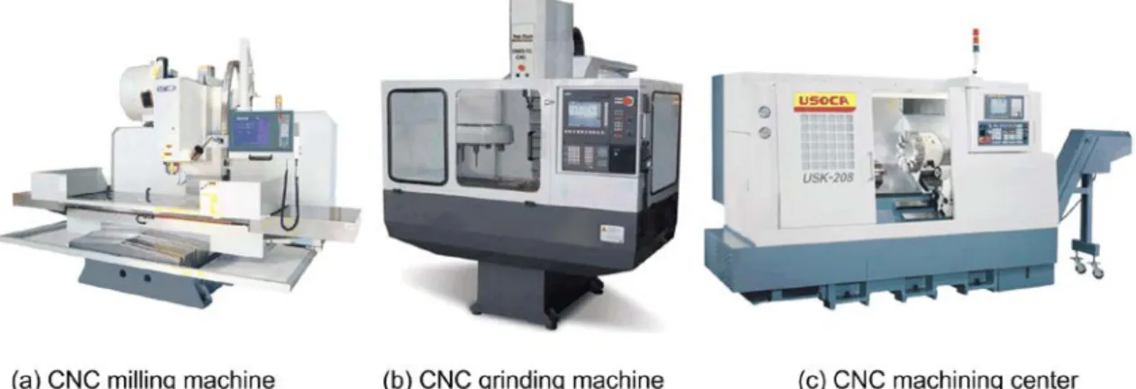
There are also some other benefits that are offered by the CNC machines and promote their wide application in industry (advanced machine control, more precise production planning due to high reputability of the machining, etc.) [30]. However, relatively high cost and limited workspace are usually treated as their main disadvantages [19]. Typical examples of CNC‐machines are presented in Figure 2.4.

Figure 2.4 Examples of CNC‐machines

Auteurs : AK, AP

implemented control algorithm and the number of actuated axes. With respect to the motion control system, the CNC‐machines may be classified as point‐to‐point and contouring ones. The first of them, also called a positioning system, moves the tool to the given location without control of the path and speed (they are not important for some applications, such as drilling). Continuous path systems ensure the path and speed control of the tool while machining, they implement simultaneous control of all driven axes. Typical application areas of continuous motion control are milling and turning.

Based on the control algorithm, the CNC‐machines are divided into open‐loop and closed‐loop ones. In the open‐loop systems, the actuator input is entirely defined by the programmed instructions and there is no feedback to check whether the desired goal (position, velocity) has been achieved. They are obviously rather sensitive to external disturbances, so their application area is limited by the cases where the accuracy requirements are not critical. In contrast, closed‐loop systems have a feedback, which allows us to compensate any differences between the desired position/velocity and its actual value. This feedback may be implemented using both analogous and digital technique, the close‐loop systems are usually considered to be very precise and attractive for accurate machining.

With respect to the third classification factor, the number of axes, the CNC‐machines with 2, 3, 4 and 5 axes are distinguished. The first of these usually have only two translational driven axes that ensure control of the tool in the plane. The 3‐axis machines are able to process more complex 3‐dimentional surfaces, they usually employ three translational drives with mutually orthogonal axes. The more sophisticated are 4‐ and 5‐ axis CNC machines that are able to change the tool orientation, in addition to translational motions. This allows to produce more complex tool path movements and to process very complicated products. In general, increasing of the number of axes provides numerous advantages such as better surface quality, reduction of the machining time, improved access to under cuts and deep pockets, etc. It is worth also mentioning that the axes may be actuated either sequentially or simultaneously, but present systems usually implement the simultaneous control.

In modern CNC systems, the machining trajectory design is highly automated and is performed in a CAD/CAM environment. It is used for creating spatial representation of a part; planning and optimization of the tool paths and cutting parameters in creating CNC code; loading, initialization, and operating the CNC‐ machine; etc. So, CAD/CAM technologies introduce essential benefits to machining such as higher productivity, reduced design time, more accurate designs, less time required for modifications, repeatability.

Hence, the CNC‐machines ensure a number of benefits for machining of high performance materials. However, for some aeronautic applications that are closely related to this research, they have rather limited workspace and are not applicable for machining of large dimensional parts. In this case, industrial robots are more attractive, so their suitability for the milling of high performance materials is considered below.

Industrial robots. For the considered application area, robots could gain all functionalities of the CNC‐ machines and are reasonable alternative for them. Also, they provide larger workspace and more flexibility [11][4][21]. Besides, emerging technologies allow robots to perform diverse manufacturing processes such as complex cutting and material removal, tapping and drilling, surface finishing and others. All these functions can be realized by the same robot, that makes it universal, while CNC‐machines can execute only one or a group of similar operations. In addition, robot‐based machining cells are applicable for secondary operations and have a relatively large working envelope, which is extremely important for large components. Such

Auteurs : AK, AP

machining cells are more flexible and allow us to produce different products at the same time, they can be also easily adopted to manufacturing of other products. They usually provide two alternative solutions to modify the tool path: (i) to change it in the CAD/CAM system, or (ii) to teach a robot in some key points. Robots are more intelligent and ensure more sophisticated motion control, and users can map their inaccuracies and compensate for them off‐line using a dedicated model (the stiffness model for instance, as in this work) [40].

In machining applications, robots often use force and torque sensors that allow online estimation of the deflections in the tool locations with respect to the desired ones. The force and torque sensors are usually integrated into a robot's wrist, and the robot controller are able to compensate these deflections via relevant calculations. However, to achieve good quality of machining process and to eliminate robots errors caused by different factors, some additional research is required [42]. This is the main issue that resists to robot applications in some areas.

With respect to their architecture, all industrial robots can be classified into two groups. First group includes robots with strictly serial architecture, which are currently the most common industrial ones. The second group put together manipulators with strictly parallel architecture and cross‐linkages [25][26]. Typical examples of robots from both groups are presented in Figure 2.5. In order to indicate advantages of both architectures let us focus on their principal features.

Figure 2.5 A serial Kuka robot (a) and an Adept parallel robots (b)

Serial robots. This type of robots is based on serial kinematic chains composed of rather rigid links connected by actuated joints. The joints may be either rotational or translational. The main advantage of serial robots is large workspace with respect to their own volume and occupied floor space. But, since serial manipulators have open kinematic structure, all errors are accumulated and amplified from link to link. Besides, it is impossible (or rather difficult) to get high stiffness and high dynamic properties simultaneously. For instance, robots with high stiffness usually are heavy and cannot provide high speed. Moreover, their own weight induces undesirable significant stresses in actuated joints that reduces allowed payload. On the other hand, serial robots with small link mass have low stiffness and cannot provide high payload because of significant compliance errors. These issues essentially decrease efficiency and application areas of such manipulators. However, some limitations related to manufacturing errors can be withdrawn by advanced control.

According to its kinematic architecture, serial manipulators can be classified into three main groups: (a) SCARA robots, (b) Articulated robots and (c) Cartesian/Gantry robots [57]. It is worth mentioning that

Auteurs : AK, AP

here they are included in articulated ones.

The SCARA acronym stands for "Selective Compliant Assembly Robot", it is also often referred to as: "Selective Compliant Articulated Robot Arm". This type of robots is based on a 4‐axis manipulator (Figure 2.6a) [9] that ensures motion to any point within its workspace (X‐Y‐Z translation) and the end‐effector rotation around the vertical axis (theta‐Z). For this architecture, the vertical Z‐motion is independent and is provided by a dedicated linear actuator, while three remaining rotational joints (with parallel axes) ensure full range of translations and rotations in XY‐plane. Because of this specific architecture (with three parallel rotational joints), SCARA is slightly compliant in the XY‐plane but is rather rigid in the Z‐direction (so called selective compliance). The selective compliant feature makes this robot highly suitable for many types of assembly operations. Due to low mass in moving parts, it provides very good dynamic properties. This promote SCARA to be ideal for pick‐and‐place, palletizing and de‐palletizing, machine loading/unloading and packaging applications, which require fast, repeatable and articulate point‐to‐point movements.

Figure 2.6 Typical architectures of serial robots

The second group includes articulated robots (Figure 2.6b) [24][3], which are also called "anthropomorphic arms". Their mechanical structure is based on rotational joints and the links are arranged in a chain. Usually the articulated robots have five or six controlled axes, while robots with seven and more actuated joints also exist. This structure provides very good kinematic dexterity, so the robots have an ability to reach the target location over obstacles and ensure almost any position and orientation of the tool within the workspace. Essential advantage of the articulated robots is that they are very compact and provide the largest workspace relative to their size. However, because of complexity of direct/inverse kinematics, their control is not trivial: when driving an articulated robot in its natural coordinate system (joint space), it is difficult to obtain a straight‐line‐motion of the end‐effector in Cartesian space. So, intensive computations are required to transform the Cartesian location into the actuated joint angles (and vice versa), but this problem is not already significant because of essential computing capacity of modern microprocessors. The capabilities of the articulated robots make them well suit for a wide variety of industrial application, including machining [31][1].

The third group includes Cartesian robots (Figure 2.6c) [8], which have almost the same kinematic architecture as conventional CNC‐machines. The main differences are in the areas of control principle, programming language and mechanical design of the end‐effector connector, which for the robots is rather universal. The mechanical structure of such robots is based on three translational actuated joints whose axes

Auteurs : AK, AP

are mutually orthogonal. Such arrangement ensures very simple control when any motion in X‐Y‐Z space is achieved by straightforward actuation of relevant joints. Cartesian robots have a rectangular workspace whose volume can be increased easily. Extremely large work envelope is ensured by Gantry robots (also belonging to the Cartesian family), where one of the horizontal translational axes is supported at both ends. Due to their mechanical structure, Cartesian robots provide high rigidity and good accuracy but their kinematic dexterity is rather limited; sometimes they cannot reach around objects. Besides, to satisfy the large workspace requirement, they need large volumes to operate and occupy essential floor space. Because of its rigidity, such robots are very attractive for machining applications, but only if the tool orientation may remain the same during processing.

Figure 2.7 Examples of parallel robots integrated in the machining cells

Parallel robots. This type of robots, which are also often referred to as parallel kinematic machines (PKM), is a closed‐loop mechanism whose end‐effector is linked to the base by several independent kinematic chains [25]. The kinematic chains are composed of several links that are connected to each other by both passive joints and actuated joints (rotational or translational). Such kinematics claim to offer several essential

advantages, like high structural rigidity, high dynamic capacities and high accuracy [44][50][51]. Another

important advantage of parallel robots is better accuracy, because here the position and orientation errors of separate kinematic chains are averaged by the end‐platform (instead of straightforward accumulation, as in serial robots). Besides, using special arrangement of kinematic chains, it is possible to ensure high stiffness and high dynamic properties simultaneously. These capabilities make the parallel robots well suitable for high‐

Auteurs : AK, AP

milling machine, Hexapod OKUMA machine, the VERNE machine, Hexapod‐Machine Mikromat 6X, Urane SX, and others [36][14][16][28][39][41].

However, parallel robots have very complex workspace and highly non‐linear relation between natural coordinates (actuated joints) and Cartesian ones. Consequently, their performances (maximum speeds, accuracy and rigidity) essentially differ from point to point and also depend on the moving directions. Other

disadvantages of parallel manipulators are their large footprint‐to‐workspace ratio (except the Tricept robot

which requires less space) and small range of motion because of parallel configuration. These are the main obstacles for the machine application of parallel robots [18][38][50].

At present, there exists a large variety of parallel manipulators, several examples are presented in Figure 2.8. Depending on the architecture, they may be divided into two groups that differ by the type of connection between the base‐platform and the serial chains [6].

The first group contains manipulators with fixed foot points and variable length struts. Most robots of this group implement the Stewart‐Gough architecture, have 6 degrees of freedom and are called Hexapods (Figure 2.9) [25]. They provide high precision and accuracy, good stiffness and high load/weight ratio. Due to these essential advantages, Hexapods are often used in flight simulators, precision machining, surgical robots, and other areas. By variation of the link lengths, Hexapods may satisfy both small and large workspace, but increasing of the link length has a direct effects on the accuracy. The main technical problem of Hexapod is high friction in the ball joints. Typical examples of parallel manipulators belonging to the first group are presented in (Figure 2.8 a‐g), they include VARIAX, HEXA, TRICEPT, TRIPOD, Delta and others [13][35][37][29][7][46][56].

The second group includes manipulators with foot points gliding on fixed linear joints. Robots of this group differ by the number of actuated translational axes and their location with respect to each other, as well as by the type of links connecting the base and moving platforms. Typically, they have 5 or 6 degrees of freedom (HEXAGLIDE, HexaM) but there are also 3 degrees of freedom translational manipulators of this family (Orthoglide) that employ parallelogram‐based links similar to Delta robots [53][6][45]. The robots of the second group (see Figure 2.8 h‐l) are attractive for machining application because of lower moving mass compared to the hexapods and tripods. However, to ensure large workspace, such robots require large volumes to operate and occupy essential floor space.

Hence, parallel robots provide essential benefits compared to the serial ones, which promote them to high speed and high precision machining applications considered in this work. For this reason, they have already been employed in commercial machining centers (see Figure 2.7) that progressively replace conventional CNC machines based on serial Cartesian architecture. A short summary of a dedicated comparison study is given below.

Auteurs : AK, AP

Figure 2.8 Typical architectures of parallel robots

Auteurs : AK, AP

Figure 2.9 Examples of Hexapod parallel kinematic machines

Résumé. Integrated results of the above analysis are summarized in Table 2.4. They show that the CNC‐ machines are quite suitable for majority of machining operations provided that a large workspace and high dynamics are not required. However, for high speed machining of relatively large parts that are widely used in the aerospace and shipbuilding industries, conventional CNC‐machines can be hardly used. In contrast, robotic manipulators are able to execute such tasks and simultaneously ensure higher flexibility of automated machining cells. The only problem with robots application is their rather low stiffness that leads to non‐ negligible position errors under the forces/torques of the technological process. Thus, the next section focuses on the robot accuracy issue.

Table 2.4 Comparison of CNC and robotic‐based machining Performance

factor Conventional XYZ CNC‐machines

Robotic‐based machining

Serial robots Parallel robots Workspace _{(by foot print)} Limited _{(limited by link lengths)} Large _{(by parallel architecture)} Limited

Flexibility Limited number of _operations Any operation in the workspace

Dynamics Low Limited High

Accuracy High Depends on the stiffness, link weights and payload Stiffness High _{accumulated along the chain} Moderate, compliance is _{stiffness is aggregated} High, separate chain

Auteurs : AK, AP

2.4 References

[1] E. Abele, M. Weigold, S. Rothenbücher, Modeling and Identification of an Industrial Robot for Machining Applications, Annals of the CIRP Vol. 56/1/2007, 387‐390

[2] Dubbel handbook of mechanical engineering, Ed. W. Beitz and K.‐H. Kuttner, Springer‐Verlag London Limited, Great Britain 1994

[3] F. Benamar, P. Bidaud, F. Le Menn, Generic differential kinematic modeling of articulated mobile robots, Mechanism and Machine Theory, Volume 45, Issue 7, 2010, Pages 997‐1012

[4] T. Brogardh, Present and future robot control development—An industrial perspective, Annual Reviews in Control 31 (2007) 69–79

[5] K. Castelino R. D’Souza and P.K. Wright, Tool‐path Optimization for Minimizing Airtime during Machining, Journal of Manufacturing Systems Vol. 22/No, 3 2003, 173‐180

[6] D. Chablat, P. Wenger, Architecture Optimization of a 3‐DOF Parallel Mechanism for Machining Applications, the Orthoglide, IEEE Transactions On Robotics and Automation 19(3) (2003) 403‐410. [7] R. Clavel (1988). DELTA, a fast robot with parallel geometry, Proceedings, of the 18th International

Symposium of Robotic Manipulators, IFR Publication, pp. 91–100.

[8] M. Dadfarnia, N. Jalili, Z. Liu, D.M. Dawson, An observer‐based piezoelectric control of flexible Cartesian robot arms: theory and experiment, Control Engineering Practice, Vol. 12, Issue 8, 2004, pp. 1041‐1053 [9] M. Taylan Das, L. Canan Dülger, Mathematical modelling, simulation and experimental verification of a

scara robot, Simulation Modelling Practice and Theory, Volume 13, Issue 3, April 2005, Pages 257‐271 [10] C. Dumas, S. Caro, M. Cherif, S. Garnier and B. Furet, A Methodology for Joint Stiffness Identification of

Serial Robots, Intelligent Robots and Systems (IROS), 2010 IEEE/RSJ International Conference on, pp. 464 ‐ 469

[11] Irene Fassi, Gloria J. Wiens,Multiaxis Machining: PKMs and Traditional Machining Centers, Journal of Manufacturing Processes, Volume 2, Issue 1, 2000, Pages 1‐14

[12] Garant machining manual, http://www.hoffmann‐group.com/download/en/ zerspanungshandbuch/en‐ zerspanungshandbuch.pdf

[13] M. Geldart, P. Webb, H. Larsson, M. Backstrom, N. Gindy, K. Rask, A direct comparison of the machining performance of a variax 5 axis parallel kinetic machining centre with conventional 3 and 5 axis machine tools, International Journal of Machine Tools and Manufacture, Vol. 43, Issue 11, 2003, pp. 1107‐1116 [14] Goto, J, Okuma Krauss‐Maffei Injection Moulding Machine‐‐OSP KM‐5000 With Computerized Numerical

Control, Jpn. Plast. Age. Vol. 23, no. 205, pp. 35‐38. Sept.‐Oct. 1985

[15] Springer handbook of mechanical engineering, Ed. K‐H Grote and E. Antonsson, Springer, New York 2009 [16] Daniel Kanaan, Philippe Wenger, Damien Chablat, Kinematic analysis of a serial–parallel machine tool:

The VERNE machine, Mechanism and Machine Theory, Volume 44, Issue 2, 2009, Pages 487‐498

[17] B. Kaya, C. Oysu, H.M. Ertunc, Force‐torque based on‐line tool wear estimation system for CNC milling of Inconel 718 using neural networks, Advances in Engineering Software 42 (2011) 76–84

[18] Kim, J., Park, C., Kim, J. and Park F.C., 1997, “Performance Analysis of Parallel Manipulator Architectures for CNC Machining Applications,” Proc. IMECE Symp. On Machine Tools, Dallas.

[19] Krause, P.C., Analysis of Electrical Machinery, New Work, McGraw‐Hill (1984)

[20] A. Lamikiz, L.N. Loґpez de Lacalle, J.A. Saґnchez, M.A. Salgado, Cutting force estimation in sculptured surface milling, International Journal of Machine Tools & Manufacture 44 (2004) 1511–1526

Auteurs : AK, AP

robot, Robotics and Autonomous Systems 54 (2006) 453–460

[22] Shih‐Wei Lin, Zne‐Jung Lee, Kuo‐Ching Ying, Chung‐Cheng Lu, Minimization of maximum lateness on parallel machines with sequence‐dependent setup times and job release dates, Computers & Operations Research 38(2011) 809–815

[23] Chih‐Ching Lo, CNC machine tool surface interpolator for ball‐end milling of free‐form surfaces, International Journal of Machine Tools & Manufacture 40 (2000) 307–326

[24] Shin‐ichi Matsuoka, Kazunori Shimizu, Nobuyuki Yamazaki, Yoshinari Oki, High‐speed end milling of an articulated robot and its characteristics, Journal of Materials Processing Technology, Volume 95, Issues 1‐3, 15 October 1999, Pages 83‐89

[25] J.‐P. Merlet, Parallel Robots, Kluwer Academic Publishers, Dordrecht, 2006.

[26] J.‐P. Merlet, C. Gosselin, Parallel mechanisms and robots, In B. Siciliano, O. Khatib, (Eds.), Handbook of robotics, Springer, Berlin, 2008, pp. 269‐285.

[27] A. Nektarios, N.A. Aspragathos, Optimal location of a general position and orientation end‐effector's path relative to manipulator's base, considering velocity performance, Robotics and Computer‐ Integrated Manufacturing, Volume 26, Issue 2, April 2010, Pages 162‐173

[28] Neugebauer, R., Wieland, F., Schwaar, M., Karczewski, Z., Hochmuth, C., Erfahrungen mit dem Mikromat Hexapod 6X (1998), Internationales Parallelkinematik‐Kolloquium 1998. Zürich: IWF ETH‐Zürich, 1998, pp. 65‐79

[29] K.E. Neumann, 1988, “Robot,” United State Patent no. 4,732,625.

[30] S.T. Newmana, A. Nassehi, X.W. Xu, R.S.U. Rosso Jr, L. Wang, Y. Yusof, L. Ali, R. Liu, L.Y. Zheng, S. Kumar, P. Vichare, V. Dhokia, Strategic advantages of interoperability for global manufacturing using CNC technology, Robotics and Computer‐Integrated Manufacturing 24 (2008) 699– 708

[31] Adel Olabi, Richard Béarée, Olivier Gibaru, Mohamed Damak, Feedrate planning for machining with industrial six‐axis robots, Control Engineering Practice, Volume 18, Issue 5, May 2010, Pages 471‐482 [32] Cuneyt Oysu, Zafer Bingu, Application of heuristic and hybrid‐GAS Aalgorithms to tool‐path optimizati on

problem for minimizing airtime during machining, Engineering Applications of Artificial Intelligence 22 (2009) 389–396

[33] C. O. Ozgur, J. R. Brown, A two‐stage traveling salesman procedure for the single machine sequence‐ dependent scheduling problem, Omega, Volume 23, Issue 2, April 1995, Pages 205‐219

[34] H. Paris, D. Brissaud, A. Gouskov, A More Realistic Cutting Force Model at Uncut Chip Thickness Close to Zero, Annals of the CIRP, 56:415‐418, 2007

[35] Pierrot, F., Dauchez, P., Fournier, A., HEXA: a fast six‐DOF fully‐parallel robot, Fifth International Conference on Advanced Robotics, 1991. 'Robots in Unstructured Environments', 91 ICAR., vol. 2 pp. 1158 ‐ 1163

[36] F. Pierrot and T. Shibukawa, From Hexa to previous termHexaM.next term In: C.R. Boër, L. Molinari‐ Tosatti and K.S. Smith, Editors, Parallel kinematic previous termmachines:next term theoretical aspects and industrial requirements, Springer‐Verlag (1999), pp. 357–364.

[37] Francois Pierrot, Vincent Nabat, Olivier Company, Sebastien Krut, Optimal Design of a 4‐DOF Parallel Manipulator, From Academia to Industry, IEEE Transactions on Robotics, vol. 25, no. 2, 2009 pp 213‐224 [38] Rehsteiner, F., Neugebauer, R., Spiewak, S. and Wieland, F., 1999, “Putting Parallel Kinematics Machines

(PKM) to Productive Work,” Annals of the CIRP, Vol. 48:1, pp. 345–350.

Auteurs : AK, AP

[39] Renault Automation Magazine, n° 21, may 1999

[40] P. Rocco, G. Ferretti, G. Magnani, Implicit force control for industrial robots in contact with stiff surfaces, Automatica, Volume 33, Issue 11, November 1997, Pages 2041‐2047

[41] Seungkil Son, Taejung Kim, Sanjay E. Sarma, Alexander Slocum, A hybrid 5‐axis CNC milling machine, Precision Engineering, Volume 33, Issue 4, October 2009, Pages 430‐446

[42] J. Sulzer, I. Kovač, Enhancement of positioning accuracy of industrial robots with a reconfigurable fine‐ positioning module, Precision Engineering, 34(2) 2010, pp. 201‐217

[43] Myriam Terrier, Arnaud Dugas, Jean‐Yves Hascoet, Qualification of parallel kinematics machines in high‐ speed milling on free form surfaces, International Journal of Machine Tools & Manufacture 44 (2004) 865–877.

[44] Tlusty, J., Ziegert, J, and Ridgeway, S., 1999, “Fundamental Comparison of the Use of Serial and Parallel Kinematics for Machine Tools,” Annals of the CIRP, Vol. 48:1, pp. 351–356.

[45] Toyama, T. et al, 1998, “Machine Tool Having Parallel Structure,” United State Patent no. 5,715,729. [46] Tsai, L.W. and Joshi, S., 2000, “Kinematics and Optimization of a Spatial 3‐UPU Parallel Manipulator,”

ASME Journal of Mechanical Design, Vol. 122, pp. 439–446.

[47] C.‐L. Tsai, Y.‐S. Liao, Prediction of cutting forces in ball‐end milling by means of geometric analysis, journal of materials processing technology 205 (2008) 24–33

[48] Veeramani,D.,Gau,Y.S.,1998.Model for tool‐path plan optimization in patch‐by‐patch machining. International Journal of Production Research 36(6), 1633–1651.

[49] Min Wan, Wei‐Hong Zhang, Systematic study on cutting force modelling methods for peripheral milling, International Journal of Machine Tools & Manufacture 49 (2009) 424–432

[50] Wenger, P., Gosselin, C. and Maille, B., 1999, “A Comparative Study of Serial and Parallel Mechanism Topologies for Machine Tools,” Proc. PKM’99, Milano, pp. 23–32.

[51] Wenger, P., Gosselin, C. and Chablat, D., 2001, “A Comparative Study of Parallel Kinematic Architectures for Machining Applications,” Proc. Workshop on Computational Kinematics, Seoul, Korea, pp. 249–258. [52] A. Werner, Z. Lechniak, K. Skalski, K. KeÎdzior, Design and manufacture of anatomical hip joint end

prostheses using CAD/CAM systems, Journal of Materials Processing Technology 107 (2000) 181±186 [53] Wiegand, A., Hebsacker, M., Honegger, M., Parallele Kanematik und Lineamotoren: Hexaglide ‐ ein

neues, hochdynamisches Werkzeugmaschinenkonzept, Technische Rundschau Transfer Nr. 25, 1996. [54] X.W. Xu, S.T. Newman, Making CNC machine tools more open, interoperable and intelligent—a review

of the technologies, Computers in Industry 57 (2006) 141–152

[55] Min Xu, R. B. Jerard and B. K. Fussell, Energy Based Cutting Force Model Calibration for Milling, Computer‐Aided Design & Applications, Vol. 4, Nos. 1‐4, 2007, pp 341‐351

[56] Dan Zhang, Lihui Wang, Conceptual development of an enhanced tripod mechanism for machine tool, Robotics and Computer‐Integrated Manufacturing, Volume 21, Issues 4‐5, 2005, Pages 318‐327

[57] http://www.robotmatrix.org/default.htm

Auteurs : AK, AP

3 STIFFNESS MATRIX OF ROBOTIC MANIPULATORS WITH

PASSIVE JOINTS

3.1 Introduction

IN many applications, manipulator stiffness becomes one of the most important performance measures of a robotic system. In particular, for milling, drilling and other types of machining, the stiffness defines the positioning errors due to interaction between the workpiece and the technological tool. Similarly, in industrial pick‐and‐place automation, the manipulator stiffness defines admissible velocity/acceleration while approaching the target point, in order to avoid undesirable displacements due to inertia forces. Other examples include medical robots, where elastic deformations of mechanical components under the task load are the primary source of positioning errors.

Numerically, this property is usually described by the stiffness matrix KC, which defines a linear relation between the translational/rotational displacement in Cartesian space and the static forces/torques causing this transition (assuming that all of them are small enough). The inverse of KC is usually called the compliance matrix and is denoted as kC. As it follows from related works, for conservative systems, KC is 6 6× semi‐definite non‐negative symmetrical matrix but in general case its structure may be non‐diagonal to represent the coupling between the translation and rotation.

The problem of stiffness matrix computing for different types of manipulators has been in the focus of robotic experts for several decades [1‐18]. The existing approaches may be roughly divided into three main groups: (i) the Finite Element Analysis (FEA) [19‐23], (ii) the Matrix Structural Analysis (SMA) [24‐28], and (iii) the Virtual Joint Method (VJM) [1‐2,8,14,29‐30]. The most accurate of them is obviously the FEA‐based technique but it requires rather high computational expenses. The SMA is less computationally hard due to fairly large structural elements employed (3D flexible beams instead of numerous tiny tetrahedrals and hexahedrals of FEA) but nevertheless it is not convenient for the parametric analysis. And finally, the VJM method is the most attractive in robotic domain since it operates with an extension of the traditional rigid model that is completed by a set of compliant virtual joints (localized springs), which describe elastic properties of the links, joints and actuators. This Chapter contributes to the VJM technique and focuses on some particularities of the manipulators with passive joints.

For conventional serial manipulators (without passive joints), the VJM approach yields rather simple analytical presentation of the desired stiffness matrix KC. Relevant expression

1 T C q q q − − = K J K J can be found in the work of Salisbury [1] who assumed that the mechanical elasticity is concentrated in actuators and the deflections are small enough to apply linear approximation of the force‐deflection relation. Here the matrix

q

K aggregates the stiffness coefficients of all elastic joints, and Jq is the corresponding kinematic Jacobian.

Further, this result was extended by Gosselin for case of parallel manipulators taking into account elasticity of other mechanical elements [2]. More recent publications present VJM‐based stiffness analysis for particular case studies, such as various variants of the Stewart–Gough platform, manipulators with US/UPS legs, CaPAMan, Orthoglide, H4 etc. [27‐34].

Auteurs : AK, AP

It should be noted that in the majority of related works, the presence of passive joints1 _{does not cause}

any specific computational problems, since these joints are eliminated via geometrical constraints describing the assembling of the relevant parallel architecture [2]. Besides, in most of publications, it is implicitly assumed that the Jacobian Jq describing influence of the elastic joints on the end‐location is non‐singular2, i.e.

( )

6

rank Jq = , to ensure inversion of the related matrix in the modified expression

(

)

1 T T C q q q q − − = K J K J that always produce non‐singular KC. It is obvious that the assumption concerning Jq is completely realistic if the VJM model includes at least a single 6‐dimensional virtual spring of a general type (see [38] for details), while it is not realistic that the manipulator stiffness matrix is always non‐singular. Hence, common stiffness modelling techniques must be revised with respect to influence of passive joints, which in certain cases can not be straightforwardly eliminated from the kinetostatic equations and, consequently, may cause singularity of KC

3_.

In this Chapter, another approach is applied that originates from our publication [30] where the desired stiffness matrix KC of size 6 6× is extracted from the inverse of a larger matrix, of size

(

6+nq

) (

× 6+nq

)

, which additionally includes the passive joint Jacobian Jq (nq is the passive joint number). Advantages of this approach and its ability to produce singular stiffness matrices were confirmed by a number of examples, but explicit analytical solution was not presented. Hence, this work concentrates on analytical computations of the stiffness matrix and also on influence of the passive joints on particular elements of KC.

It is also worth mentioning that some previous works [30] propose (or at least discuss) a trivial solution of the considered problem, which deals with a straightforward modification of the matrix Kq, in accordance

with the passive joint type and geometry (corresponding rows and columns are set to zero). However, as it will be shown below, this straightforward approach gives true results if (and only if) the matrix Kqis diagonal, but

it is not valid in general case where there is a coupling between different types of the elementary virtual springs presented by non‐diagonal coefficients.

The remainder of this Chapter is organised as follows. Section 4.2 presents a simple motivation example that confirms the problem non‐triviality. Then, Sections 4.3 and 4.4 propose relevant analytical solutions for a serial kinematic chain and a parallel manipulator respectively. Section 4.5 focuses on computational issues and proposes recursive procedure and a set of corresponding analytical rules. Section 4.6 contains application

1 _{It should be mentioned that here passive joints have stiffness equal to zero and they should be distinguished from}

passive compliant joints studied by other authors, whose stiffness is nonzero.

2 _{It is important to distinguish the conventional kinematic Jacobian}

J, which is computed with respect to actuated

coordinates and may be both singular and non‐singular, and the Jacobian Jq that is computed with respect to the virtual

springs coordinates and is always non‐singular. Besides, they differ in sizes, which for a standard serial 6‐d.o.f.

manipulator are respectively 6x6 and 6 36× .

3 _{The main problem with straightforward application of the classical expression} 1 1

( T)

C q q q

− −

=

K J K J to the manipulators

with passive joints is related to the invertibility of the matrix Kq, which becomes singular if stiffness of some virtual

springs is assign to zero (to describe the passive joint properties). In fact, there are two sequential inversions here applied to singular matrices that may be treated similarly to an indeterminate form "1/(1/0)" in calculus that finally produces 0, but cannot be obtained numerically. So, finally, double inversion of singular matrix should produce another singular matrix, but numerical computations obviously fails. To overcome this difficulty and to solve the problem in a rigorous way, our previous publication [30] proposes a dedicated technique that deals with inversion of non‐singular matrices of higher dimension and extraction from them relevant 6x6 sub‐matrix.

Auteurs : AK, AP

main results and gives prospective for future work.

3.2 Motivation example

Let us present first a simple example that demonstrates non‐trivial transformation of the stiffness matrix due to the presence of passive joints. For the purpose of simplicity, let us limit our study to 2D Cartesian space and consider a single manipulator link, which is assumed to be fixed at the one end. It is also assumed that the external loading (the forces ,F Fx y and the torque Mz) is applied to another end; either directly or through a passive joint.

Under these assumptions, the elastostatic properties of the link can be described by a symmetrical stiffness matrix K=  Kij of size 3 3× and its potential energy due to elastic deformations (linear deflections

,

x y

δ δ and angular deflection δϕ) may be expressed as

(

)

[

]

11 12 13 21 22 23 31 32 33 , 1 · 2 , · · K K K x x y x y K K K y K K K E δ δ δ δϕ δ δ δϕ δ δϕ              =    (3.1)

If the link is equipped with a passive joint, the energy of this mechanical system (link with passive joint) must be minimized with respect to the joint variable4_{. For instance, in the case of the rotational passive joint}

z

R allowing free rotation around the z‐axis at the reference point, the potential energy should be rewritten as

(

,

)

min

(

, ,

)

p x y E y

E x

δϕ

δ δ = δ δ δϕ (3.2)

and the passive joint variable δϕ may be expressed via the remaining coordinates as

13 23 33

(K x K y) /K

δϕ= − δ + δ . Then, after relevant transformations and computations of the second‐order derivatives (i.e. the Hessian of Ep with respect to x, y and ϕ)

2 2 11 12 3 2 2 3 2 / , / ,... / p p p p p p K = ∂ E ∂x K = ∂ E ∂ ∂x y K = ∂ E ∂ ϕ (3.3)

the desired stiffness matrix of links with passive joint may be expressed as

13 31 32 13 11 12 33 33 23 31 23 32 21 22 33 33 · · 0 · · 0 0 0 0 p K K K K K K K K K K K K K K K K                   − − = − − K (3.4)

This expression clearly shows that, if the matrix K is non‐diagonal, a trivial transformation that was proposed in some previous works (i.e., simple setting to zero of the third row and column) does not produce a truthful result. Moreover, the elements of the upper‐left 2 2× block must be modified taking into account the

4 _{It is worth mentioning that in novel compliant robotics systems it may be required to maximise the potential energy}

storage in order to exploit/recycle it to improve energy efficiency [40] [41]

Auteurs : AK, AP

elements of K that are located outside of this block. Similar results corresponding to other types of passive joints are summarized in Table 3.1, where they are also applied to classical 2D beam (in this case, some elements of the Kp are four times lower compared to K ). This conclusion motivates development of a general methodology of the stiffness matrix transformation, which is presented below.

Table 3.1 Transformation of the link stiffness matrix due to passive joints (2D case)

Auteurs : AK, AP