Stability and Consistency of the LISP
Pull Routing Architecture
Yue Li
∗, Damien Saucez
‡, Luigi Iannone
∗, Benoit Donnet
†∗ Telecom ParisTech – France
‡ Université Côte d’Azur, Inria – France
† Université de Liège, Montefiore Institute – Belgium
Abstract—Future Internet has been a hot topic for the lastdecade. One of the approaches put forward in order to revise the Internet architecture is LISP – Locator/ID Separation Protocol, which leverages the separation of the identifier and the locator roles of IP addresses. Contrary to the classical push model used by the BGP-based routing architecture, LISP relies on a pull model. In particular, routing information is pulled from a new network element, the Mapping System, to provide the association between the identifier (i.e., the address used to identify a host inside a domain) and a list of locators (i.e., the addresses to locate an attachment point) upon an explicit query. In this paper, we evaluate a LISP Mapping System deployment in the public LISP Beta Network from two standpoints: Stability and Consistency. Our measurements show that the mapping information is stable over time and consistent between the different mapping entities and the vantage points. Our analysis shows that there are cases where the Mapping System is unstable and/or inconsistent, hence, beside proposing a taxonomy in order to classify them, we carry out an in-depth investigation of such cases so to provide hints on how to improve the performance of LISP.
Index Terms—LISP, experiment, measurement I. INTRODUCTION
Our economy relies so much on the Internet that multihom-ing and interdomain traffic engineermultihom-ing became a must have. Unfortunately IP and the routing protocol of the Internet, i.e., BGP, are poorly designed to cope with mobility, multihoming, and complex traffic engineering requirements [1]. To over-come the fundamental limitations of BGP, several solutions have been proposed aiming at redesigning the actual Internet architecture [2], some of them being based on the principle of the locator/identifier separation paradigm.
Among the various proposals of locator/identifier separation mechanism, the Locator/ID Separation Protocol (LISP) [3] is being developed by the Internet Engineering Task Force (IETF). Its philosophy is to split the current IP addressing space into two roles, namely identifiers and locators, where each role has only one specific semantic, while avoiding introducing any new address format. In LISP, an identifier used to identify a communicating endpoint is called EID (Endpoint IDentifier), which can be used as source/destination addresses in a local domain, i.e., within the LISP-sites. A locator, called RLOC (Routing LOCator), refers to an attachment point in the Internet topology, which is used to route on the Internet core. The separation of addressing space requires LISP to have a mapping system able to bind identifiers and locators together. In particular, such bindings (or mappings) are pulled
in an on-demand fashion from the mapping system, in order to obtain the information necessary to establish end-to-end communication.
The globally routable nature of RLOCs avoids the need for the Internet core (also known as Default Free Zone – DFZ) to change any routing mechanism. The EID is used inside the stub networks for local forwarding and does not cause any change in the routing mechanism either. The separation is able to simplify the management of routing tables for network entities in the Internet as well as in the local scope, since the size of routing tables is reduced. Internet core routers do not need anymore to maintain the routes towards the stub networks and stub networks do not any longer need to know the routing information of the core Internet [4].
The mapping between RLOCs and EIDs is the cornerstone of LISP and a deep study on the performance of LISP mapping system is essential. Thus, we leverage the LISP Beta Network, where LISP has been deployed in the wild for seven years [5], to conduct measurement campaigns. Such a worldwide real playground has been used to assess the state of LISP deployment and how it has evolved over the years [6]. It has also been used to evaluate interworking between LISP and non-LISP sites [4]. The preliminary analysis, however, does not indicate the maturity of the LISP mapping system. In this paper, we propose a much deeper study and a more thorough evaluation, focusing on the exploration of all mapping systems on LISP Beta Network through active LIG (LISP Internet Groper [7]) measurement. The temporal comparison shows that the mapping system is quite stable over time and the crosswise comparison indicates that the mapping system is consistent between network entities. However, some instability and cases of inconsistency are also identified through evalua-tion. Thus, we propose a taxonomy to classify and investigate them in depth to offer feedback to forward LISP technology. The remainder of this paper is organized as follows. Sec. II provides the necessary background about LISP and the cur-rent LISP Beta network deployment. Sec. III presents an overview of the experiment campaigns and introduces the metrics that we use to evaluate the performance of mapping system. Sec. IV and Sec. V respectively describe the mapping system stability and consistency results in details, by using the proposed taxonomy, and investigate in depth the causes from different viewpoints. Finally, Sec. VI concludes the paper summarizing our main findings.
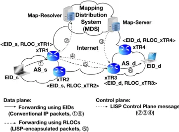
Internet AS_s AS_d Mapping Distribution System (MDS) EID_s EID_d <EID_s, RLOC_xTR2> <EID_s, RLOC_xTR1> <EID_d, RLOC_xTR3> <EID_d, RLOC_xTR4> Map-Resolver Map-Server
Data plane: Control plane: Forwarding using EIDs
(Conventional IP packets, !") Forwarding using RLOCs (LISP-encapsulated packets, #)
LISP Control Plane message ($%&) ! $ % & # " xTR1 xTR2 xTR3 xTR4
Fig. 1. LISP data and control plane packet forwarding sequence.
II. LISP BACKGROUND
The Locator/IDentifier Separation Protocol (LISP) [3], [8] separates traditional IP addressing space into two logical addressing spaces: (i) the Endpoint IDentifier space (EID); (ii) the Routing LOCator space (RLOC). The EID space is an IPv4 or IPv6 address used as source and/or destination address, playing the role of host identifier in stub-networks (called LISP-sites). The hosts within the same LISP site can com-municate with each other using EIDs, since EIDs are locally routable. The RLOC space is an IPv4 or IPv6 address used on the upstream interface of the border router located between the LISP-site and the provider. Communications beyond the local domain (i.e., other LISP-sites or the legacy Internet), need to encapsulated in packets using RLOCs addresses, since RLOCs are globally routable. As a result, the destination and source EIDs are in the inner packet header, while the destination and source RLOCs are in the outer header. Packet encapsulation and forwarding is performed by the LISP Data Plane. Binding EIDs to RLOCs, so to actually make encapsulation possible, is the responsibility of the LISP Control Plane. The synergy between LISP Control and Data planes guarantees end-to-end communication, encapsulating conventional IP packets in LISP packets as well as correctly forwarding them through the core Internet. The details about their operation are described respectively in Sec. II-A and Sec. II-B. It is followed by an overview of LISP Beta network (Sec. II-C), which is the world-wide LISP platform.
A. LISP Data Plane
The LISP Data plane mainly takes care of the encapsulation and decapsulation operations done at the source and destina-tion networks. LISP basically provides a level of indirecdestina-tion through a tunneling mechanism over the core Internet (the so called Default-Free Zone – DFZ), as shown in Fig. 1, in order to provide end-to-end communication. More specifically, any host willing to communicate with another host, uses its own
EID as source address and the EID of other host as destination address to generate regular IP packets. These packets are first transferred as usual to the border router, called Ingress Tunnel Router (ITR) (as the 1st step show in Fig. 1). Then the ITR encapsulates the regular IP packets into a LISP packet by adding a tunnel header [3], where the RLOC of ITR is used as source address and the destination RLOC as destination address. After encapsulation, the LISP packets are forwarded over the Internet core (the 5th step in Fig. 1). When arriving at the destination border router, called Egress Tunnel Router (ETR), the LISP packets are decapsulated (i.e., the tunnel header is removed) and transferred to the destination host (the 6th step in Fig. 1). The solid line in Fig. 1 indicates packets forwarding using EID address space, while the dashed line presents using the RLOC space. A device which acts as both an ITR and an ETR is denoted as xTR.
B. LISP Control Plane
The LISP Control plane is mainly tasked to associate EIDs with RLOCs, i.e., perform a mapping. A new network entity named mapping system is introduced by LISP to perform such EID-to-RLOC mapping. In particular, a mapping contains an EID prefix and an associated list of <RLOC, Priority, Weight> tuples. The RLOC with the highest priority is preferred. The weight is taken into account only to perform load balancing in the case of several RLOCs having the same priority.
Mappings are stored in two data structures on xTRs: the LISP Database and the LISP Cache. The LISP Database is populated by configuration and stores all known EID-to-RLOC mappings, for which the EID-Prefixes are behind the xTR. On an ITR, this helps selecting a source RLOC for an EID used in encapsulation. While on an ETR, it is used to verify whether itself is the proper ETR connecting to the destination EID, so that such ETR is able to forward the decapsulated packets to the final destination. The LISP Cache temporally stores mappings for the EID-prefixes of the remote communicating end-points. On an ITR, it is used to select the destination RLOC of the outer header of the LISP-encapsulated packet. While on an ETR, it is used to perform a basic anti-spoof verification. Different from the LISP Database, the LISP Cache is populated on demand. The procedure is triggered by the first packet of a new flow, which can not find a suitable mapping for the destination EID among the mappings stored in the LISP Cache. The mappings in the LISP Cache are purged if not used upon expiration of a timeout ([9], [10], [11], [12]).
The current BGP-based Internet routing architecture relies on a push model, in which routing information is pushed to the whole Internet. LISP-based routing instead relies on a pull model where routing information is pulled only when actually needed. This paradigm shift requires making routing information available in an on-demand manner. To achieve this purpose, the LISP Control plane introduces a new sys-tem: the Mapping Distribution System (MDS) to provide a mapping upon an explicit query.1 The work-flow of the MDS 1The terms Mapping Distribution System (MDS) and mapping system are used interchangeably in this paper.
is illustrated with dotted line in Fig. 1. If an ITR cannot find a mapping in LISP Cache for a new flow, it sends a query, called Map-Request, to a Map-Resolver (MR) [13]. The MR is a network node that determines whether the queried destination IP address is an EID. If not, a Negative Map-Replyis returned; otherwise, the query is forwarded by the MR within the MDS according to the specific protocol/architecture, towards the Map-Server (MS). The MS is a network device that learns EID-Prefix mapping entries (a list of EID-Prefixes plus a set of <RLOC, Priority, Weight> tuples) from ETRs. Then MS forwards the query to the xTR that registered the mapping for the requested EID. The xTR in turn directly sends a Map-Reply message containing the requested mapping to the ITR initiating the query. Map-Resolvers offers an interface of MDS to the xTRs, so that the whole complex MDS mechanism can be hided. At the time of this writing, only two mapping systems have been implemented: LISP Alternative Topology (LISP+ALT [14]) and LISP Delegated Database Tree (LISP-DDT [15]), with the latter actively deployed.
C. LISP Beta Network
LISP has been deployed in the Internet since 2008 [5]. Started as the only LISP testbed, LISP Beta network had a steady growth and achieved world-wide experimental de-ployment [6] with the purpose to gain real-life experience on LISP. The members of LISP Beta Network are not only academics, research laboratories, and startups offering LISP related services, but also major companies and operators. Par-ticipants of this network are located in 34 different countries, with the highest concentration in Europe and North America. Due to a monolithic control by one single commercial actor, however, LISP Beta network has limitations to explore the innovative services. Thus, some other projects, such as ANR LISP-Lab project [16], are under implementation to develop new enhanced features.
LISP Beta Network has 13 available MRs/MSes at the moment. In March 14th 2012, the mapping system used by LISP Beta Network has switched from LISP+ALT [14] to the more flexible LISP-DDT [15].Changing the mapping system has considerably reduced the configuration and maintenance burden, while a slight performance degradation has been observed [6]. LISP Beta Network consists of 518 LISP sites. Although the deployment scope is still limited compared to the Internet, its size is sufficient to conduct reasonable measurement campaigns to understand LISP behavior and performance. The measurement results presented hereafter are collected through this experimental platform, especially focusing on its mapping system.
III. METHODOLOGY
In order to collect data to carry out our analysis, several measurements campaigns have been performed. Hereafter we provide an overview on the measurements and the metrics used in our evaluation.
A. Measurements Overview
To obtain a comprehensive and in-depth evaluation of LISP Beta Network Performance, we conducted experiments using a tool called LIG (LISP Internet Groper [7]). This management tool is used to query the LISP mapping system. When LIG is launched, a Map-Request is sent for a destination IP address, and the returned Map-Reply is then stored for further analysis. There are three possible types of Map-Reply mes-sages: (i) LISP Map-Reply, where the reply contains mapping information to reach the LISP-enabled sites; (ii) Negative Map-Reply, where the reply states that the requested IP address belongs to a prefix of a non-LISP site; (iii) No Map-Reply, where no answer is received within some amount of time. A query is considered to be successful if either a LISP Map-Reply or a Negative Map-Reply is received. A query is considered to be failed if No Map-Reply is received within 5 seconds.
The experiments are conducted from July 2nd to 18th 2013. From a set of different vantage points (VPs), we used LIG to send Map-Request messages to all the Map-Resolvers of the LISP Beta Network, for all selected destination IP addresses every 30 minutes. The set of VPs was composed by part of academic networks, commercial Internet, PlanetLab and spread across Europe and USA. The destination IP addresses consisted of the first address within each prefix regardless of the type (i.e., the EID-prefixes or regular prefixes), derived from the LISPmon project [17]. The latter is a LISP Beta net-work monitoring site that periodically crawls the IP addressing space, through the MDS, to discover all the prefixes used as EID addressing space. During this measurement campaign, 5 VPs and 13 MRs/MSes were available and 613 EIDs were queried in total.
In this paper, we analyse the Map-Replies associated with EIDs instead of all regular IP addresses. In the remainder of this paper, we use the term experiment round to identify a complete Map-Request/Map-Reply exchange by LIG for all the selected destinations to all the available MRs over all existing VPs. Although No Map-Reply occasionally appears in some experiment rounds, since it does not contain any mapping information, we just focus on LISP Map-Reply and Negative Map-Reply to conduct the analysis.2
B. Metrics
As indicated in Sec. II-B, the LISP Control plane is in charge of offering the mapping information that consists of an EID-prefix associated with a list of <RLOC, P riority, W eight> tuples. Theoretically, unless configuration has changed, if the same EID-prefix is queried, Map-Replies should always contain the same mapping in-formation, no matter from which VP the query is sent, and no matter which MR is queried. During our measurements, however, we found that the Map-Replies are not always identical as they are supposed to be. The reasons causing the Map-Reply changes are summarized in Table I.
2We use “simultaneously” or “at the same time” as synonym of “at a same experiment round”.
TABLE I MAP-REPLYDIFFERENCES
Category Mismatch
Map-Reply Type Negative Map-Reply and LISP Map-Reply
RLOC set RLOC number RLOC address RLOC priority RLOC weight RLOC state
The Map-Reply differences can be classified into two broad categories: the first is a difference in terms of Map-Reply Type, which means that a mix of Negative Map-Reply and LISP Map-Reply occurs; the other type of difference is in the RLOC set, which means that at least one of the attributes associated with RLOC set is different. More specifically, RLOC number indicates a difference in the number of RLOC tuples received in the Map-Reply. The others are differences in a RLOC tuple, which consists of RLOC address, RLOC priority, and RLOC weight (presented in Sec. II-B).3 The RLOC state is derived from the R-bit in Map-Reply message, which is set when the sender of a Map-Reply has a route to the RLOC, meaning that from its viewpoint the RLOC is up and running. If at least one of the six parameters shown in Table I conveyed in a Map-Reply is different from the previous one (over time) or the others (between different VPs or MRs) at the same experiment round, the Map-Reply is marked as different. Based on the criteria of the Map-Reply difference, we propose two metrics to evaluate in more details the performance of the LISP mapping system: (i) Stability and (ii) Consistency.
A mapping is considered to exhibit stability if the Map-Replies for one specific EID obtained from one MR observed at a given VP (briefly denoted as a tuple <EID, M R, V P >), over time, are identical. A classification taxonomy for unstable cases is proposed later in Sec. IV.
A mapping is considered to exhibit consistency if: i) Map-Replies for a specific EID from all MRs observed at a given VP (denoted as a group <EID, ∗, V P >) are identical at the same time (this kind of consistency is referred as Consistency by MR); ii) Map-Replies for a specific EID-MR pair in all VPs (denoted as a pair <EID, M R, ∗>) are identical at the same time (referred as Consistency by VP). A classification taxonomy for non-consistent cases is proposed later in Sec. V.
IV. MAPPINGSYSTEMSTABILITYEVALUATION
In this section, we study the stability of the mapping system over time. More precisely, we consider that an EID is stable if all mappings retrieved for this EID are identical. If it is not the case, we say there is instability.
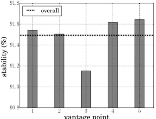
Overall, when we consider the whole dataset, 91.49% of observations are stable, which indicates that over the full set of observations, changes are infrequent and the MDS is stable. When the stability is considered on a per vantage point basis, we observe, as shown in Fig. 2, that the stability is 3The terms RLOC address and RLOC are used interchangeably in this paper.
1 2 3 4 5 vantage point 90.8 91.0 91.2 91.4 91.6 91.8 st ab ili ty (% ) overall
Fig. 2. Overall percentage of stability observed at five different VPs.
0 10 20 30 40 50 instability frequency (%) 91 92 93 94 95 96 97 98 99 100 cd f( % )
Fig. 3. CDF of instability frequency. X-axis is instability frequency, indicating the ratio of instability occurrence number for one <EID, M R, V P > tuple over total experiment number.
independent of the vantage point since no significant deviation from the overall average can be observed (dashed line in Fig. 2). Nevertheless, while these results demonstrate that the mapping system is generally stable, in the following of this section, we investigate the reason why about 8.51% of the observations exhibit instability.
Fig. 3 complements Fig. 2 by showing, for each tuple <EID, M R, V P >, the frequency f<EID,M R,V P > at which mappings are different, by using the following definition:
f<EID,M R,V P >=
# Instabilities
# Experiments × 100%. (1)
Thus, if the instability frequency f<EID,M R,V P > is 0%, it means that such a tuple is always stable during the whole experiment, i.e., its Map-Replies are always the same. On the contrary, a tuple <EID, M R, V P > with instability frequency of 100% indicates that its current Map-Reply is never identical to the previous ones, i.e., its Map-Replies change at every experiment round.
Fig. 3 shows the CDF of the mapping changes frequency (i.e., instability frequency). It shows the probability where the instability frequency equals to zero is 91.49%, which is coherent with the result in Fig. 2 (dashed line) and means the mapping is globally stable. This CDF also shows that, for the mapping changes case, 82.77% (98.53−91.49100.0−91.49%) of all mapping changes events have an instability frequency less
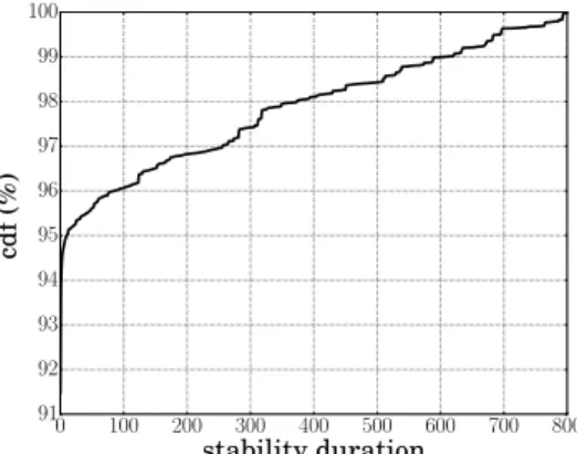
0 100 200 300 400 500 600 700 800 stability duration 91 92 93 94 95 96 97 98 99 100 cd f( % )
Fig. 4. CDF of stability duration (in number of rounds). X-axis is stability duration, indicating during how many experiment rounds that the mapping for one <EID, M R, V P > tuple is stable.
TABLE II
PERCENTAGE OFINSTABILITIES BYCATEGORY
New Deployment Statistical outliers Mobility Reconfiguration
72.36% 7.23% 0% 20.41%
than 1%. We can deduce that mapping changes, if they occur, are rare events. The existence of instability frequency around 50% means that, in some cases, even though it is rather rare, the mapping changes occurs almost one time every two experiment rounds.
While Fig. 3 indicates that mappings can potentially change frequently, Fig. 4 shows the CDF of the stability duration, i.e., for how many experiment rounds a mapping remains stable. We observe that the majority of instabilities has a stability duration of 1 experiment round. This fact shows that the mapping change occurs during each measurement period (i.e., 30 minutes, the interval between two experiment rounds). At the other side of the curve, stability lasts up to 800 experiment rounds are observed, indicating that the mapping changed at the very beginning of or the end of the measurements we performed. In the dataset we identified both cases for such situations. To further understand the instability, we classify it into four categories:
• New Deployment: the Map-Replies of a tuple
<EID, M R, V P > mix two different types: Negative Map-Reply and LISP Map-Reply.4
• Statistical outliers: the Map-Replies of a tuple <EID, M R, V P > change more frequently than usually seen. In our measurements, outliers corresponds to mappings that change at least 3 times during a day. • Mobility: the Map-Replies of a tuple <EID, M R, V P >
are explicitly tagged with the mobility bit as specified in RFC6830 [3].
• Reconfiguration: all cases that fit neither into the New Deployment case nor the Statistical outliers case. 4It is caused more often by turning on/off the xTRs than the real deployment of LISP sites. Since the consequence of Map-Reply changes between Negative Map-Reply and LISP Map-Reply, we make this case named New Deployment.
0.4 0.5 0.6 0.7 0.8 0.9 1.0 dissimilarity 0 20 40 60 80 100 cd f( % )
Fig. 5. CDF of the dissimilarity among different types of instabilities.
Tab. II presents the percentage of observations for the four categories. New Deployments dominate the total unstable cases with a percentage of 72.36%, followed by Reconfig-uration with 20.41%, and Statistical outliers with 7.23%. Throughout the dataset, we did not observe any Mobility event, probably due to the fact that the mobility specifications were not yet implemented at the time of measurements. Therefore, we omit the Mobility category in the rest of this paper.
New Deployments are the most common instabilities and we used spectral analysis with Fourier transforms and auto-correlation to understand if such events are correlated between themselves. This analysis shows that New Deployments are equally spread over the whole measurement period, i.e., their occurrence per day is relatively constant. We performed the same study on the Reconfiguration category and Statistical outliers and reached the same conclusion, i.e., the absence of correlations between events.
Since New Deployments are incidental events that can happen at any time, no particular duration is observed for this category of instabilities. Moreover, as New Deployments account for 72.36% of instabilities, it significantly impacts the duration distributions shown in Fig. 4, explaining the relatively smooth evolution of the CDF. On the contrary, Statistical outliers are characterized by very frequent changes and they bias the distribution around the lowest duration values, explaining the relatively high number of observations for small duration.
To characterize the mapping changes happening during instabilities, we derived the following dissimilarity metric d(mi, mj) = 1 − |m|mi∩mj|
i∪mj|, based on the Jaccard similarity
coefficient, where mxis the RLOC set of mapping x. A dis-similarity of 1 indicates that no RLOCs are shared between the two compared mappings, while a dissimilarity of 0 indicates that the RLOC sets are the same. Fig. 5 shows the CDF of the mappings’ dissimilarity for each unstable <EID, M R, V P > tuple. In our experiment, the dissimilarity results are discrete (as the discrete points shown in the Fig. 5) in a range from 0.33 to 1.0. As one can expect, the most likely dissimilarity is 1 in 90.09% of the total number of instabilities. These observations mostly come from New deployment case where before turning on the xTR, no RLOC is provided with the Negative
Reply (RLOC set is empty), hence, switch to a LISP Map-Reply implies a full change in the RLOC set. As 90.09% is larger than the 72.36% of New deployments share, it indicates as well that complete change of the RLOC set have also been observed during Reconfiguration and Statistical outliers. For the rest, no particular trend can be observed showing that changes of RLOC set can actually take any form.
V. MAPPINGSYSTEMCONSISTENCYEVALUATION
In this section, we discuss the consistency of the mapping system respectively by MR and by VP. More precisely, we consider that a tuple of <EID, ∗, V P > exhibits consistency, if all the Map-Replies from different MRs, for a certain EID, observed at a given VP are identical at the same time (same experiment round). This kind of consistency is denoted as consistency by MR. Similarly, if all the Map-Replies sent by a specific MR, for a certain EID, and observed at different VPs are identical at every experiment round, then we consider that a tuple of <EID, M R, ∗> is consistent, and denote it as consistency by VP. Otherwise, for cases not falling in the above two, we simply say that there exists inconsistency.
Overall, throughout the whole dataset, we found that 86.3% of observations of all <EID, ∗, V P > tuples are consistent, which indicates that non-identical Map-Replies from different MRs are uncommon. Similarly, consistency by VP is observed in 90.48% of observations of all <EID, M R, ∗> tuples, showing that the Map-Replies received at different VPs are usually identical. In the following, Sec. V-A will go deeper in the analysis of consistency by MR, proposing as well several types of inconsistency; then Sec. V-B will provide thorough analysis of consistency by VP.
A. Consistency Evaluation by MR
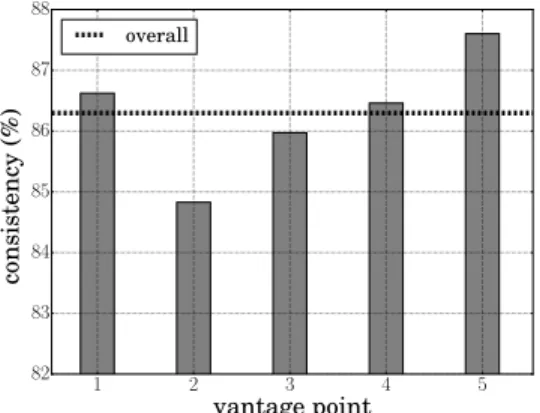
The overall percentage of consistency by MR is 86.3% (see the dashed line on Fig. 6), meaning that across the whole experiment traces the inconsistency among the Map-Replies sent by different MRs is not common. Yet, we can also observe from Fig. 6 that different VPs show some deviations from the overall consistency by MR, reflecting the fact that while certain VPs receive the same Map-Reply from different MRs, some other VPs receive inconsistent responses. Such deviation is very small (no more than 2.77%) among different vantage points, indicating that it remains a relatively rare event. These results show that the mapping system is consistent among different MRs in general, but the inconsistency exists at the same time with a percentage around 13.7%. In the remainder of this section, we go deeper this issue, exploring the reasons why the few observations exhibit inconsistency by MR.
We compute the CDF of the inconsistency frequency by MR f<EID,∗,V P >, i.e., the probability of inconsistency fre-quency over all <EID, ∗, V P > tuples, by using the following definition:
f<EID,∗,V P > =
# Inconsistencies by MR
# Experiments × 100%. (2)
For a <EID, ∗, V P > tuple, an inconsistency frequency of 0% means that all Map-Replies from all of the different MRs for
1 2 3 4 5 vantage point 82 83 84 85 86 87 88 co ns is te nc y (% ) overall
Fig. 6. Overall consistency by MR at 5 different Vantage Points.
0 20 40 60 80 100 inconsistency frequency by MR (%) 82 84 86 88 90 92 94 96 98 100 cd f( % )
Fig. 7. Cumulative Distribution Function of inconsistency frequency by MR. X-axis is inconsistency frequency by VP, indicating the ratio of inconsistency occurrence for each <EID, ∗, V P > tuple over total experiment number.
one EID are the same at each experiment round throughout the whole measurement campaign. For a <EID, ∗, V P > tuple, an inconsistency frequency of 100% means that at each experiment round during the whole measurement campaign, there is at least one MR replying a Map-Reply different from the replied by other MRs. The resulting CDF of inconsistency frequency is shown on Fig. 7. The value 0% of inconsistency frequency has a probability of 82.38%, indicating that through all the dataset, there are 82.38% of <EID, ∗, V P > tuples that are always consistent by MR at whichever VP. Yet, it is worth noticing that this value is lower than the overall consistency of 86.3% shown in Fig. 6. The reason of such difference lays in the fact that, when we analyze the 0% inconsistency frequency, we just take into account those common EIDs exhibiting a consistency by MR in all VPs. Hence 82.38% represents the subset of the EIDs considered in the former percentage and is the lower bound, guaranteeing that 82.38% of <EID, ∗, V P > tuples always have consistent responses, regardless at which VP. In addition, the inconsistency frequency concentrates at a very low range, since a sharp increase occurs between 0% and 2% with a growth of 16.15% (98.53% - 82.38%). It indicates that the <EID, ∗, V P > tuples classed as inconsis-tent do actually receive inconsisinconsis-tent responses rarely, hence, demonstrating that the mapping system is generally consistent. Yet, in very few cases (only 0.5%), the inconsistency between different MRs occurs all the time.
So far, the analysis indicates that the mapping system is consistent by MR in general, but the inconsistency indeed exists. To have a closer look to the inconsistency, we further cluster it into two cases:
Map-Reply Type: The type of Map-Reply provided by the 13 MRs for a specific <EID, ∗, V P > tuple is different, meaning that some MRs provide LISP Map-Reply while others return a Negative Map-Reply. The difference of received Map-Reply type leads the xTRs to use a different way to send the packets, i.e., xTRs receiving a LISP Map-Reply sends LISP-encapsulated packets by using the obtained RLOCs, while xTRs receiving a Negative Map-Reply will forward the conventional packets (i.e., without LISP-encapsulation).
RLOC set: All the Map-Replies returned by the 13 MRs for a <EID, ∗, V P > tuple belong to LISP Map-Reply type, but the associated attributes (cf. Tab. I from Sec. III) are different. For instance, some Map-Replies may contain RLOC1, while some others convey RLOC2 (i.e., the RLOC address is not identical); or some Map-Replies have only one RLOC, whereas others have multiple RLOCs (i.e., the RLOC number is different), and so on. The difference in such Map-Replies could lead the requesting xTRs to select different destination RLOCs. The large majority of inconsistencies, around 98.34%, are Map-Reply Type, probably because there is an update of mapping information in the mapping system for the New Deployment case. Not all of the 13 MRs simultaneously update the mapping information, meaning that a convergence time is needed so that the global mapping information maintained in all parts of the mapping system is synchronized. If VPs query the mapping system during this convergence period, some MRs will still provide Negative Map-Replies, while other (already updated) MRs will forward the Map-Requests towards the corresponding ETRs, which in turn will send the updated LISP Map-Replies, and vice versa. This situation contributes to the inconsistency frequency around 1%, which means that there is an inconsistency once or twice between Map-Replies from different MRs for one specific EID, since changing the status of xTR is not frequent.
Just few inconsistencies, only 1.66%, are caused by the RLOC set. This scenario usually occurs for those EIDs whose RLOCs change frequently over time (the case of Statistical outliers instability). So, because of the convergence time of the mapping system, it is very difficult to guarantee that every MR can provide the same LISP Map-Reply at every experiment round. This reason for changes in the RLOC set is most probably due to traffic engineering policies. Similarly as the previous case, when different MRs provide a different RLOC set for a specific EID, the requesting xTRs may end up using different RLOCs to reach the same destination EID.
B. Consistency Evaluation by VP
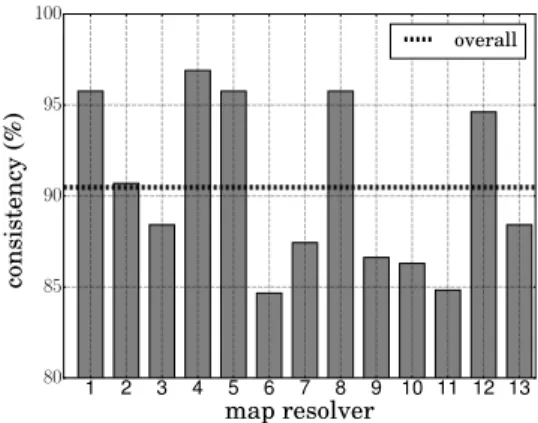
The overall percentage of consistency by VP for the whole experiment dataset is 90.48%, presented by the dotted line in Fig. 8, which indicates that the Map-Replies received
1 2 3 4 5 6 7 8 9 10 11 12 13 map resolver 80 85 90 95 100 co ns is te nc y (% ) overall
Fig. 8. Overall consistency by VP from the different Map-Resolvers.
0 10 20 30 40 50 60 inconsistency frequency by VP (%) 85 90 95 100 cd f( % )
Fig. 9. Cumulative Distribution Function of inconsistency frequency by VP. X-axis is inconsistency frequency by VP, indicating the ratio of inconsistency occurrence for each <EID, M R, ∗> tuple over total experiment number.
at different VPs from the same MR are highly consistent. Yet, we can also observe that different MRs show some deviations from the overall consistency by VP, reflecting the fact that certain MRs send the same Map-Reply to all VPs, but some do not. The deviation among different MRs is however limited (less than 12.23%). Therefore, we can certainly state that the mapping system shows generally a high degree of consistency by VP but presents a non-negligible amount of inconsistencies (9.52%). In the rest of this section, following the same approach as for the consistency by MR, we go deeper into this issue, exploring the reasons why some observations exhibit inconsistency by VP.
Fig. 9 shows the CDF of the inconsistency frequency by VP f<EID,M R,∗>, i.e., the probability of inconsistency fre-quency for all <EID, M R, ∗> tuples, by using the following definition:
f<EID,∗,V P >=
# Inconsistencies by VP
# Experiments × 100%. (3)
As same as the explanation for Fig. 7, here an inconsistency frequency by VP of 0% means that all Map-Replies received by all of the VPs from a same MR are totally consistent at ev-ery experiment round during the whole experiment campaign, while an inconsistency frequency of 100% means that at least one of VPs received an inconsistent Map-Reply compared to the other VPs at every experiment round. The probability of
consistency by VP (when X-axis is 0% in Fig. 9) is similar to that by MR, with a value of 81.57%. It can be noticed that this percentage is slightly lower than the overall percentage of consistency by VP in Fig. 8. The reason is that here the inconsistent occurrence with 0% only includes those EIDs for which all VPs always show consistency, no matter which MR is actually queried. A sharp increase with a growth of 16.97% (98.53% - 81.56%) is found when X-axis is 1%, which means that although VPs sometimes receive inconsistent Map-Replies at several experiment rounds, the occurrence remains pretty low, hence showing that even by VP the mapping system exhibits a very high degree of consistency. Differently from the largest inconsistency frequency by MR, which goes up to reaches 100%, the largest inconsistency frequency by VP is only 66%. This phenomenon indicates a fact that the Map-Replies received by different VPs are not inconsistent all the time, at least there are one third of observations show that their Map-Replies are totally same. Thus the consistency by VP is higher than consistency by MR.
To further explore the inconsistency by VP, we then use same metrics as in Sec. V-A, with the exception that the queried target changes from <EID, ∗, V P > to <EID, M R, ∗> tuples.
The most inconsistent case, 89.06%, is due to a mix of Negative Map-Reply and LISP Map-Reply, i.e., demand for a same <EID, M R, ∗> tuple, at some VPs receive Negative Map-Reply but at others receive LISP Map-Reply. This is caused by the New Deployment case, but differently from the cause for inconsistency by MR, the reason for inconsistency by VP is probably because of Map-Requests sent by different VPs can not be processed exactly at the same time, due to queuing in the MR. Thus, if the queries are sent during the period of mapping information update, some VPs, whose Requests are processed first will have different Map-Reply Type from the latter ones. Inconsistencies caused by different RLOC sets, i.e., different VPs receive LISP Map-Replies with different RLOCs set from the same MR, also exist, contributing for around 10.94%. It is probably caused by a combination of the Statistical outliers instability case and the queuing mechanism in MR. As the RLOC sets provided by a MR for some certain EIDs frequently change, and the Map-Requests sent by different VPs need to be processed one by one, it is very possible that the first processed Map-Requests are replied by the different RLOC sets compared to the latter ones. The difference between Map-Replies is probably due to traffic engineering policies, but the further experiments are needed to explore the deeper reasons for such inconsistency.
VI. CONCLUSION
As a solution to cope with the increase of BGP routing table, traffic engineering, and scalability issues, LISP has been deployed on the LISP Beta Network experimental testbed since 2008. To ensure accurate and efficient communications, the mapping system, which is the corner stone of the LISP architecture, should be stable and consistent. For the purpose of evaluating stability and consistency of the LISP mapping
system, we measured the LISP Beta Network for seventeen days. Measurements show that the LISP mapping system is stable and consistent over time. Nevertheless, cases of instability and inconsistency are observed, which we classified in a newly proposed taxonomy. All in all, instability and inconsistency are rare events. Meanwhile, we also provide possible reasons causing the instability and inconsistency, but the further experiments are needed to prove them.
Acknowledgments: Research work presented in this paper is supported by the French Research Agency under ANR-13-INFR-0009 LISP-Lab Project (www.lisp-lab.org) and benefited support from NewNet@Paris, Cisco’s Chair "NETWORKS FOR THEFUTURE" at Telecom ParisTech (http://newnet. telecom-paristech.fr). Any opinions, findings or recommendations expressed in this material are those of the author(s) and do not necessarily reflect the views of partners of the Chair.
REFERENCES
[1] B. Quoitin, L. Iannone, C. De Launois, and O. Bonaventure, “Evaluating the benefits of the locator/identifier separation,” in Proc. ACM/IEEE International Workshop on Mobility in the Evolving Internet Architecture (MOBIARCH), August 2007.
[2] H. Naderi and B. E. Carpenter, “A review of IPv6 multihoming so-lutions,” in Proc. 10th International Conference on Networks (ICN), January 2011.
[3] D. Farinacci, V. Fuller, D. Meyer, and D. Lewis, “The locator/ID separation protocol (LISP),” Internet Engineering Task Force, RFC 6830, January 2013.
[4] F. Coras, D. Saucez, L. Iannone, and B. Donnet, “On the performance of the LISP beta network.”
[5] “LISP Beta Network,” see http://www.lisp4.net.
[6] D. Saucez, L. Iannone, and B. Donnet, “A first measurement look at the deployment and evolution of the Locator/ID separation protocol,” ACM SIGCOMM Computer Communication Review, vol. 43, no. 1, pp. 37–43, April 2013.
[7] D. Farinacci and D. Meyer, “The locator/ID separation protocol Internet groper (LIG),” Internet Engineering Task Force, RFC 6835, 2013. [8] D. Saucez, L. Iannone, O. Bonaventure, and D. Farinacci, “Designing
a deployable Internet, the locator/IDentifier separation protocol,” IEEE Internet Computing, vol. 16, no. 6, pp. 14–21, November/December 2012.
[9] L. Iannone and O. Bonaventure, “On the cost of caching locator/id mappings,” in Proceedings of the 2007 ACM CoNEXT conference. ACM, 2007, p. 7.
[10] J. Kim, L. Iannone, and A. Feldmann, “A deep dive into the LISP cache,” in Proc. IFIP Networking, May 2011.
[11] H. Zhang, M. Chen, and Y. Zhu, “Evaluating the performance on IDLoc mapping,” in Proc. IEEE Global Communications Conference (GLOBECOM), November 2008.
[12] F. Coras, A. Cabellos-Aparicio, and J. Domingo-Pascual, “An analytical model for the LISP cache size,” in Proc. IFIP Networking, May 2012. [13] V. Fuller and D. Farinacci, “Locator/ID separation protocol (LISP)
map-server interface,” Internet Engineering Task Force, RFC 6833, January 2013.
[14] V. Fuller, D. Farinacci, D. Meyer, and D. Lewis, “Locator/ID separation protocol alternative logical topology (LISP+ALT),” Internet Engineering Task Force, RFC 6836, January 2013.
[15] V. Fuller, D. Lewis, and A. Ermagan, V. Jain, “LISP Delegated Database Tree,” Internet Engineering Task Force, Internet Draft, Work in Progress draft-ietf-lisp-ddt-01.txt, March 2013.
[16] “LISP-Lab,” August 2016, see http://www.lisp-lab.org. [17] “LISPmon,” August 2016, see http://www.lispmon.net.