HAL Id: hal-00703382
https://hal.inria.fr/hal-00703382v2
Submitted on 4 Jun 2012HAL is a multi-disciplinary open access
archive for the deposit and dissemination of sci-entific research documents, whether they are pub-lished or not. The documents may come from teaching and research institutions in France or abroad, or from public or private research centers.
L’archive ouverte pluridisciplinaire HAL, est destinée au dépôt et à la diffusion de documents scientifiques de niveau recherche, publiés ou non, émanant des établissements d’enseignement et de recherche français ou étrangers, des laboratoires publics ou privés.
Reduced Dependent Ordered Binary Decision Diagrams:
An Extension of ROBDDs for Dependent Variables
Raymond A. Marie
To cite this version:
Raymond A. Marie. Reduced Dependent Ordered Binary Decision Diagrams: An Extension of ROB-DDs for Dependent Variables. [Research Report] RR-7984, INRIA. 2012, pp.18. �hal-00703382v2�
0 2 4 9 -6 3 9 9 IS R N IN R IA /R R --7 9 8 4 --F R + E N G
RESEARCH
REPORT
N° 7984
May 2012Ordered Binary Decision
Diagrams:
An Extension of ROBDDs
for Dependent Variables
RESEARCH CENTRE
RENNES – BRETAGNE ATLANTIQUE
An Extension of ROBDDs for Dependent
Variables
Raymond A. Marie∗
Project-Team Dionysos
Research Report n° 7984 — May 2012 — 18 pages
Abstract: In this report, we presented an extension of robdds that is able to accommo-date certain dependencies among their (Boolean) variables. In particular, this extension shows evidence of being applicable to evaluating the dependability (reliability, availabil-ity) of systems whose structures are representable by a Boolean function. This extension consists of three main parts. The first part is the notion of a phratry with its associated new definitions and constraints. The second part consists of the adaptation and com-plementation of the original rules used in the construction of robdds. The final part concerns additional custom-made steps needed to determine the functional valuations that are specific to solving measure in question.
Key-words: ROBDDs, Binary decision diagrams, Analytical models, Fault tolerant systems, Correlation, Failure analysis, Nonindependent component analysis.
Diagrammes de décision binaire ordonnés, dépendants et
réduits :
une extension des ROBDDs pour la prise en compte de
dépendances
Résumé : Ce document présente une extension des robdds destinée à prendre en compte certaines dépendances entre leurs variables booléennes. Cette extension est particulière-ment utile pour évaluer la sûreté de fonctionneparticulière-ment (fiabilité, disponibilité) de systèmes dont la structure est représentable par une fonction booléenne et où des probabilités sont associées aux états. Cette extension est composée de trois parties. La première corre-spond à la notion de fratrie, avec ses définitions et ses contraintes. La seconde partie consiste à adapter et compléter les règles initiales utilisées dans les robdds. la troisième partie concerne les étapes spécifiques au problème à résoudre afin d’obtenir les valuations particulières aux fratries.
Mots-clés : ROBDDs, diagramme de décision binaire ordonné, système tolérant aux fautes, analyse de composants dépendants, corrélation.
1
Introduction
A Binary Decision Diagram (bdd) is a data structure that is used to represent a Boolean function on a computer. Its advantage is that it is a compressed representation permitting the execution of operations without any decompression step. The basic idea underlying the notion of a bdd is the Shannon decomposition formula of a Boolean function F (x, y, z, ...):
F(x, y, z, ...) = x.Fx=true(x, y, z, ...) + x.Fx=f alse(x, y, z, ...)
Recurrent use of this formula permits representation of a Boolean function as a binary-tree with only two types of leaf nodes corresponding respectively to the Boolean values true and false, each internal node being labeled with a Boolean variable.
The success of this approach is due to the fact that a theoretical binary-tree can be transformed into a rooted, directed, acyclic graph. In turn, this graph can be reduced through recurrent use of two fundamental rules. This reduction results in a much simpler data structure that still represents the initial Boolean function. This reduction works only if the original bdd is ordered, i.e., if the different Boolean variables appear in the same order on all the paths going from the root to the leaves. This condition is not restrictive and such a bdd is called an Ordered bdd. The final graph is normally called a Reduced Ordered Binary Decision Diagram (robdd), although many people just say bdd when they refer to the latter.
The bdd originated in logic studies for the manipulation and computation of logical expressions and were used very early in the domain of switching circuit design. Initial efforts were those of Lee [1] and Akers [2], followed by those of Bryant [3][4] who emphasized the use of a bdd as a fundamental data structure. Then came the applied domains of Computer Aided Design for VLSI and of reliability (either from Reliability Block Diagrams, or directly from Boolean expressions, or from Fault Tree representations) ([8], [9], [12]).
A limitation of this approach is the a priori condition that the different Boolean vari-ables are mutually independent. Very often, this assumption is reasonable, e.g., when working in the domain of pure logic. But in certain practical applications such as the evaluation of system dependability, this condition may not be acceptable.
Quite often, in dependability studies, Boolean variables represent states of hardware/ software elements (such as “functioning/not functioning”). In such studies, probabilities are affected to the two possible values of the variables: P(xi = true) = 1− P(xi = f alse).
For different reasons, complex systems may contains several groups of correlated indi-vidual elements in the sens of dependability properties. In that case, P(xi | xj) 6= P(xi) and
we cannot valuate the outgoing edges of node labeled by Boolean xi if we don’t know the
value of Boolean xj. But respectively, since (P(xi | xj) 6= P(xi)) ⇒ (P(xj | xi) 6= P(xj)),
we cannot valuate the outgoing edges of node labeled by Boolean xj if we don’t know
the value of Boolean xi. In that case, we are facing a deadlock when trying to use the
classical bdd approach. For small populations of correlated elements, we may determine a personalized model for the specific system. But the problem stays for coping with several groups of arbitrary size and with arbitrary location of the elements in the structure of the system. Moreover, in many situations, the joint probability distribution P(xi, xj) depends
4 Raymond Marie
on a (time) parameter and we have to consider probability distribution functions such as P(xi, xj, t).
The purpose of this paper is to present an extension of the robdd concept so as to handle dependencies such as this. One of the characteristics of the proposed extension is that all the components sharing a dependent behavior need to be considered in a proper suborder such that no other component can be included inside this proper suborder. In addition, the two traditional rules used to reduce a classical robdd will need to be extended in order to cope with the existence of correlated failures.
The paper is organized as follows, beginning in Section 2 with some background con-cerning robdds and how they differ from the proposed extension. Section 3 is then devoted to the presentation of the extension, per se. In turn, Section 4 describes an example il-lustrating its application, followed by a concluding section that summarizes the paper’s contribution.
2
Background
The purpose of this section is two-fold. First, it provides a brief review of robbds for those who are not familiar with this concept. Secondly, it aims to help the reader understand the difference between the now classic robdd and the extension proposed herein, referred to as an rdobdd.
Except for the leaves, each node of a bdd has an out-degree of two, where the two outgoing edges are called the low edge and the high edge of the node. A function low(u) (respectively high(u)) gives the name of the node connected to node u by the low-edge (respectively. high-edge).
It is important to understand that in a bdd, each node corresponds to a Boolean function defined by the subtree initiated from that node. Let us consider a node ni labeled
by a Boolean variable xj. The Boolean function F (ni) associaded with node ni can be
expressed in terms of the Boolean functions asociated with the two successor nodes in the following way:
F(ni) = xj.F(high(ni)) + xj.F(low(ni))
F(high(ni)) is obtained from F (ni) by assigning the Boolean variable xj to the true
value, i.e., F (high(ni)) = Fxj=true(ni). Similarly, F (low(ni)) = Fxj=f alse(ni). With
respect to node ni, the node connected to it by its high-edge (respectively, low-edge) is
called its high node (respectively low-node).
The reduction of the binary tree is accomplished by applying the following two rules: R1: Merge any isomorphic subgraphs.
R2: Eliminate any node whose two children are isomorphic.
This set of reductions transforms the binary tree into a rooted directed acyclic graph that still represents the original Boolean function. Rule R1 preserves a unique repre-sentation of a unique Boolean sub-function. Rule R2 simply exploits the fact that if F(high(ni)) = F (low(ni)), then F (ni) = F (high(ni)) = F (low(ni)) so that the node ni
can be removed from the graph. These two rules are applied repeatedly as long as they’re Inria
applicable. Also, in graphical representations of the binary tree or of the rooted directed acyclic graph, the high-edge is drawn with a solid line while a dotted line is used for the low-edge. A nice property of an robdd is that any given Boolean function has, for a given ordering of the variables, a unique robdd (referred as its canonical form).
But the practical interest in obdds relies on the existence of efficient algorithms that have been implemented in software packages. These are now available within the scientific community and several of them can be found on the Web (see, for example, [13], [14], [15], [16], [17], [18], [19]).
However, it is well known that the resulting robdd depends on the chosen ordering of the variables and, since the number of possible orderings of a set of n variables equals n!, the determination of a “good" variable order (where the number of nodes is reasonably close to optimal) is still an open problem (see [10], for example). Nevertheless, some heuristic methods, based on particular types of applications, already exist ([5], [6]). In addition, there are some recent studies that employ dynamic reordering, based for example on symmetry detection and shifting ([11]).
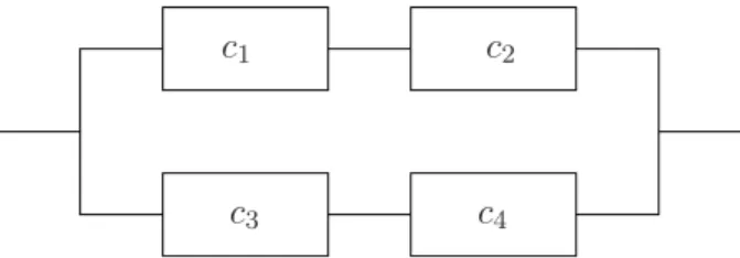
Let us now examine an application of this methodology to the simple series/parallel reliability block diagram given by Figure 1. This reliability block diagram means that the system is able to execute it function only if components c1 and c2 are not broken or/and
if components c3 and c4 are not broken. Introducing the four Boolean variables xi, i =
1, ..., 4, where xi represents the state of component ci, allows us to write the corresponding
Boolean function characterizing the reliability of the system: F (x1, ..., x4) = x1.x2+ x3.x3.
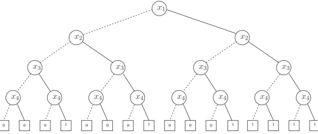
Then, from this Boolean function, we obtain the ordered bdd by recurrent application of Shannon’s decomposition theorem to the ordered sequence x1 < x2 < x3 < x4. This
ordered bdd is shown in Figure 2.
c1 c2
c3 c4
Figure 1: Series/parallel reliability block diagram
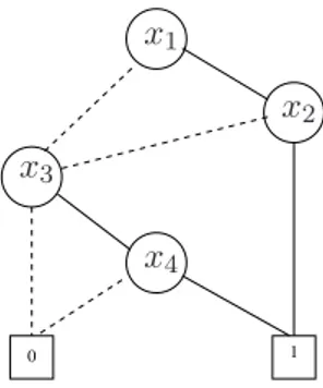
Then, using rule R1, we first merge all the isomorphic subgraphs which appear in this ordered bdd; the resulting graph is illustrated by Figure 3. In this figure, we see that there are several nodes whose two children are isomorphic. Using rule R2, we eliminate these nodes. This action produces the graph given by Figure 4. The last step consists of merging, respectively, all the 0-terminal nodes and all the 1-terminal nodes. This last step could have been made earlier (by application of rule R1) but we postponed this reduction for the sake of legibility of the overall process. The resulting robdd is shown in Figure 5 (for the order x1 < x2 < x3 < x4).
In many applications and, in particular, dependability evaluations, we do not use the 0-terminal node and the ingoing edges of this node. Consequently, we cut the “dead” part
6 Raymond Marie 0 0 0 1 0 0 0 1 0 0 0 1 1 1 1 1 x1 x2 x2 x3 x3 x3 x3 x4 x4 x4 x4 x4 x4 x4 x4
Figure 2: Ordered bdd of the example for the order x1 < x2 < x3< x4
0 1 0 1 x1 x2 x2 x3 x3 x4 x4 x4
Figure 3: Merging isomorphic subgraphs
0 1 0 1 x1 x2 x3 x4
Figure 4: Eliminating any node whose two children are isomorphic
0 1
x1
x2
x3
x4
8 Raymond Marie
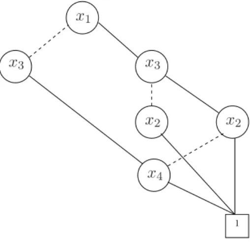
of the robdd in order to keep only what we call the “positive” robdd. This gives us the graph shown in Figure 6. We could have also been tempted to call this final graph a Zero-Suppressed robdd but this term already exists for an important type of data structure referred to as a zdd. The latter was introduced by S. Minato [7] and is able to manipulate families of sets.
To emphasize the fact that the resulting robdd depends on the chosen ordering of the variables, Figure 7 depicts the positive robdd of the example for the order x1 < x3 <
x2 < x4. Comparing it with the one in Figure 6, we see that it has two extra nodes.
Note, however, that all the Boolean expressions obtained with different variable orders correspond to the same Boolean function.
1
x1
x2
x3
x4
Figure 6: Positive robdd of the example for the order x1 < x2 < x3< x4
1 x1 x2 x2 x3 x3 x4
Figure 7: Positive robdd of the example for the order x1 < x3 < x2< x4
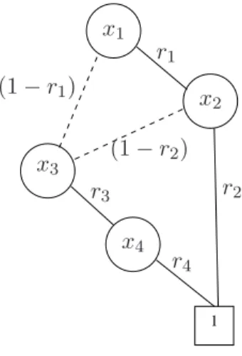
Most of the time in dependability applications, the edges of a positive robdd are valued by elementary probabilities. These probabilities correspond generally to reliabilities or to Inria
availabilities. From the point of view of robdds, these individual values are trivial since they consist of input data associated with an outgoing edge of a node and the name of the variable labeling that node. This remains so, even if their determination in a previous problem was not trivial! For our simple series/parallel example, if ri denotes
the reliability of component ci, the edge-valued robdd is shown in Figure 8 for the order
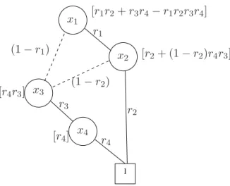
x1 < x2 < x3 < x4. Then, starting from the 1-terminal node, we compute the partial
reliability function at each node, respecting the inverse order since we cannot compute the function of one node before treating its successors. For our simple example, we get, after a final simplification, the reliability function as illustrated in Figure 9:
R(x1, x2, x3, x4) = r1r2+ r3r4− r1r2r3r4
Of course, the positive robdd associated with the order x1 < x3 < x2 < x4 yields the
same answer, again after a final simplification.
Let us add that, for several application domains where we are only interested in positive robdds, we could use an additional initial rule R0: "Eliminate the dead sub-trees," i.e., those with only 0-terminal nodes as leaves. Indeed, in many dependability applications, it is easy to avoid constructing the majority of the dead sub-trees, just by examining the Boolean structure function which indicates whether the system under consideration is up or down as a function of the up-down values of its components. For example, a Boolean variable xj appears in all the monomials of the Boolean structure function if that
component cj is in series in the reliability block diagram of the structure. Consequently,
for any node ni labeled by the Boolean variable xj, the subtree issued from the low-edge
is a dead subtree. Therefore, knowing the components in series in the reliability block diagram will allows us to avoid the construction the associated dead subtrees.
1 x1 x2 x3 x4 r1 r2 r3 r4 (1 − r1) (1 − r2)
Figure 8: Positive robdd of the example for the order x1 < x2 < x3 < x4, with elementary
10 Raymond Marie 1 x1 x2 x3 x4 r1 r2 r3 r4 (1 − r1) (1 − r2) [r1r2+ r3r4− r1r2r3r4] [r2+ (1 − r2)r4r3] [r4r3] [r4]
Figure 9: Positive robdd of the example for the order x1 < x2 < x3 < x4 with answers
(within brackets) from the bottom-up algorithm.
3
The extension
Due to the existence of subsets of Boolean variables corresponding to subsets of dependent components, we need to introduce new entities and new rules so as to evaluate dependability measures via a bdd approach.
We first distinguish a special set of Boolean variables as follows.
Definition 3.1. A phratry is a set of Boolean variables corresponding to a subset of mutually dependent components. Its cardinality equals that of the subset of components involved in a given dependence relation.
Accompanying this concept is the first of several additional rules called for by the extension.
Rule R0a(ordering rule): For every phratry, the chosen variable order must be such that the Boolean variables of a phratry are successive.
Definition 3.2. If xi1< xi2 < ... < xim corresponds to the chosen order for the Boolean
variables of a phratry Fi with cardinality m, the Boolean variable xi1 (respectively xim) is
called the eldest (respectively the benjamin) of the phratry. By extension, a node labeled by the eldest (respectively the benjamin) of the phratry is called an eldest node (respectively a benjamin node).
Definition 3.3. In an obdd, a macro-edge is a labeled and valuated edge linking an eldest node to a successor node of a benjamin node belonging to the same phratry, and such that the benjamin node belongs to the subtree of the obdd associated with the considered eldest node.
Definition 3.4. The label of a macro-edge is the sequence of 0 and 1 values characterizing the sub-path connecting the eldest node to the successor node. The 0s and 1s corresponding Inria
respectively to the low-edges and high-edges of the sub-path. Used when necessary, the valuation of the macro-edge corresponds to the dependability measure associated with the label (i.e., to the values of the Boolean variables of the phratry).
Note that for a given phratry, several macro-edges (with different labels) may have the same valuation.
In a classic robdd, the edges are valued by elementary dependability parameters, so that we don’t really have to deal with these parameters during its construction. Here, however, determination of the valuations of the macro-edges is not trivial. For this reason, we will hereby refer to them as non-trivial valuations.
Rule R0b: Eliminate the “dead” sub-trees.
This can be done by examining the corresponding Boolean structure function, as noted earlier with regard to constructing a positive obdd.
Rule R0c(phratry reductions): Replace the sub-paths of a phratry by macro-edges. Note that the application of rule R0c may transform the binary tree into a n-ary tree. Due to the existence of the macro-edges, we now need to redefine the notion of isomor-phic subgraphs.
Definition 3.5. Two subgraphs are isomorphic if they have the same topology and the same nontrivial valuations (if any).
The next rule is identical to the former rule R1 but uses the new definition of isomorphic subgraphs.
Rule R1: Merge any isomorphic subgraphs,
The former rule R2 cannot be stated as before, it needs to be adapted to existence of macro-edges.
Rule R2a: If the Boolean variable labeling the node does not belong to a phratry, then eliminate any node whose two children are isomorphic.
Rule R2b: If the Boolean variable labeling the node do belongs to a phratry, and if n, n ≥ 2, (outgoing) macro-edges are directed to the same subgraph, then replace the n macro-edges by a unique macro-edge whose valuation equals the sum of the valuations of the previous n macro-edges.
4
Example
In order to put the introduced rules in concrete form, let us consider a toy example: the series/parallel reliability block diagram shown in Figure 10. The components c11 and c12
are identical (as are the elements c21 and c22) but here the breakdown of one element
may stress the other one. In the figure, the dependence between elements is indicated by means of a "D" and of zig-zag edges connecting the dependent elements. According to the figure, there are two phratries: {x11, x12} and {x21, x22}. We consider the ordered
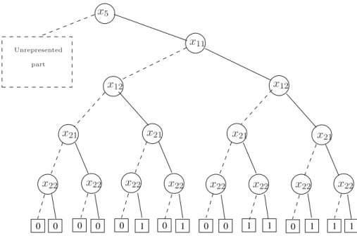
sequence x5 < x11< x12< x21< x22 (respecting rule R0a) and the corresponding ordered
bdd whose interesting part is shown in Figure 11.
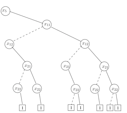
Following rule R0b, we eliminate the dead sub-trees in order to obtain the “positive” part of the bdd (cf. Figure 12).
12 Raymond Marie c11 c21 c12 c22 c5 D D
Figure 10: Series/parallel reliability block diagram of the example
0 1 1 1 0 0 0 0 0 0 1 0 1 0 1 1 x5 x11 x12 x12 x21 x21 x21 x21 x22 x22 x22 x22 x22 x22 x22 x22 Unrepresented part
Figure 11: Partial representation of the bdd
1 1 1 1 1 1 1 x5 x11 x12 x12 x21 x21 x21 x22 x22 x22 x22 x22
Figure 12: Eliminating of the dead sub-trees (rule R0b)
Next, we undertake the phratry reductions (rule R0c) consisting of three steps. The first one, very simple, is the replacement of the sub-paths of a phratry by macro-edges with their labels (cf. figure 13).
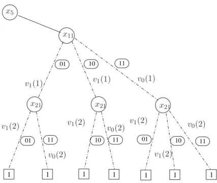
The second step is more complex since we have to assign the valuations of the macro-edges. Each valuation corresponds to the value of the dependability measure associated with the label of each macro-edge. In our example, the dependability measure is the transient probability that the elements of the phratry are in the states characterized by the label of the macro-edge. Note that, because of symmetries, macro-edges with different labels may have the same valuation.
Let F1 and F2 respectively denote the two phratries {x11, x12} and {x21, x22}. Let
vi(j), i = 0, 1, ... denote the different valuations associated with the different macro-edges
of phratry j, j = 1, 2. Here, each valuation vi(j) corresponds to a transient probability.
The determination of these different valuations needs to be done by someone familiar with dependability studies. Because the two elements of a phratry are here identical, the transient probabilities associated with labels 01 and 10 are also identical (for each of the two phratries). As a consequence, for phratry j, j = 1, 2, we use v0(j) to denote the
valuation of macro-edge with label 11 (no down element) and v1(j) to denote the valuation
of the two macro-edges associated with labels 01 and 10 (one down element) (cf. Figure 14).
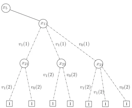
The final step of the phratry reductions consists just in dropping the labels since they are no more useful (cf. Figure 15).
14 Raymond Marie 1 1 1 1 1 1 10 01 10 11 10 1 11 01 11 01 11 x5 x11 x21 x21 x21
Figure 13: phratry reductions - labeling (rule R0c)
1 1 1 1 1 1 10 01 10 11 10 01 1 11 11 01 11 x5 x11 x21 x21 x21 v0(1) v1(1) v 1(1) v0(2) v0(2) v0(2) v1(2) v1(2) v1(2) v1(2)
Figure 14: Phratry reductions - valuating (rule R0c)
1 1 1 1 1 1 1 x5 x11 x21 x21 x21 v0(1) v1(1) v1(1) v0(2) v0(2) v0(2) v1(2) v1(2) v1(2) v1(2)
Figure 15: Phratry reductions - dropping the labels (rule R0c)
Then we are ready to apply rule 1 and merge the isomorphic subgraphs. On this example, two nodes labeled with the Boolean variable x21 are the roots of two isomorphic
subgraphs (note that the nontrivial valuations are identicalfor the two subgraphs). There are also several isomorphic subgraphs consisting of just 1-terminal nodes. Applying rule 1 for all these isomorphic subgraphs, we have the graph given by Figure 16.
We see that nodes labeled by Boolean variables x11 and x21 have isomorphic children
but since these two Boolean variables are members of phratries, we use rule 2b to merge the (outgoing) macro-edges. We finally obtain the graph shown in Figure 17.
Finally, exploiting the graph of the rdobdd given by this figure, we get the reliability expression of the structure:
R(t) = r5(t) [2v1(1) (v0(2) + v1(2)) + v1(1) (v0(2) + 2v1(2))]
where the expressions of the non-trivial valuations are supposed to be obtained from the specialist.
Although no similar rule exists in regular robdd, it might be of interest, in the appli-cation domain of dependability evaluation, to add a final rule that would eliminate nodes with single ingoing and single outgoing macro-edges. This rule would be written as:
Rule R3: Eliminate any node with single ingoing and single outgoing macro-edges and take the product of the two nontrivial values as the nontrivial value of the new macro-edge. Let us remark that, from a formal point of view, it would be necessary to enlarge the definition of the macro-edge in order to introduce this last rule, allowing the new object macro-edge to represent a set of states of more than one phratry.
16 Raymond Marie 1 1 x5 x11 x21 x21 v0(1) v1(1) v1(1) v0(2) v1(2) v0(2) v1(2) v1(2)
Figure 16: Merging isomorphic subgraphs (rule R1)
1 1 x5 x11 x21 x21 v0(1) 2v1(1) v0(2) + v1(2) v0(2) + 2v1(2)
Figure 17: Aggregating macro-edges (rule R2a)
5
Conclusion
In this paper, we presented an extension of robdds that is able to accommodate certain dependencies among their (Boolean) variables. In particular, this extension shows evidence of being applicable to evaluating the dependability (reliability, availability) of systems whose structures are representable by a Boolean function. This extension consists of three main parts. The first part is the notion of a phratry with its associated new definitions and constraints. The second part consists of the adaptation and complementation of the original rules used in the construction of robdds. The final part concerns additional custom-made steps needed to determine the functional valuations that are specific to solving measure in question.
Despite the extra difficulty introduced by the existence of macro-edges and despite the extra effort in obtaining the functional valuation, we believe that this approach is potentially useful for several classes of applications.
References
[1] C. Y. Lee. Representation of Switching Circuits by Binary-Decision Programs. Bell Systems Technical Journal, 38, pages 985 – 999, 1959.
[2] Sheldon B. Akers. Binary Decision Diagrams. IEEE Transactions on Computers, C-27(6), pages 509 – 516, June 1978.
[3] Randal E. Bryant. Graph-based algorithms for Boolean function manipulation. IEEE Transactions on Computers,C-35(8), pages 677 – 691, 1986.
[4] Randal E. Bryant. Symbolic Boolean manipulation with ordered binary-decision dia-grams. ACM Computing Surveys,24(3), pages 293 – 318, September 1992.
[5] S. Minato, N. Ishiura and S. Yajima. Shared Binary Decision Diagram with Attributed Edges for Efficient Boolean Function Manipulation. in ACM/IEEE Proc. 27th DAC, pages 52 – 57, 1990.
[6] M. Fujita, Y. Matsunaga and T. Kakuda. On Variable Ordering of Binary Decision Diagrams for the Application of Multi-level Logic Synthesis. in Proc. the European Conference on Design Automation, pages 50 – 54, 1991.
[7] S. Minato. Zero-suppressed BDDs for set manipulation in combinatorial problems. in ACM/IEEE Proc. 30th Design Automation Conf., pages 272 – 277, 1993.
[8] Stacy A. Doyle, and Joanne B. Dugan. Dependability Assessment using Binary De-cision Diagrams. in Proc. 25th International Symposiom Fault-Tolerant Computing, pages 249 – 258, 1995.
[9] M. Bouissou. An Ordering Heuristic for Building Binary Decision Diagrams from Fault Trees. in Proc. 1996 Annual Reliability and Maintainability Symposiom, pages 208 – 214, 1996.
18 Raymond Marie
[10] Beate Bollig, and Ingo Wegener. Improving the Variable Ordering of OBDDs Is NP-Complete. IEEE Transactions on Computers, C-45(9), pages 993 – 1002, September 1996.
[11] N. Kettle and A. King. An Anytime Algorithm for Generalized Symmetry Detection in ROBDDs. IEEE Transactions on Computer-Aided Design of Integrated Circuits and Systems, 27(4), pages 764 – 777, April 2008.
[12] Xinyu Zang, Hairong Sun, and Kishor S. Trivedi. A BDD-Based Algorithm for Re-liability Evaluation of Phased Mission System. IEEE Transactions on ReRe-liability,48, pages 50 – 60, 1999.
[13] F. Somenzi. CUDD: Colorado University Decision Diagram package. Available: http://vlsi.colorado.edu/ fabio/CUDD/.
[14] J. Lind-Nielsen. BuDDy: A BDD package. Available: http://sourceforge.net/projects/buddy/.
[15] Biddy: multi-platform academic BDD package, University of Maribor, Slovenia. Avail-able: http://lms.uni-mb.si/biddy/.
[16] A. Biere. The ABCD package, Johannes Kepler Universität, Linz. Available: http://fmv.jku.at/abcd/.
[17] The Berkeley CAL package, Berkeley. Available: http://embedded.eecs.berkeley.edu/Research/cal\bdd/.
[18] The JavaBDD package. Available: http://javabdd.sourceforge.net/.
[19] The Vahidi’s JDD package. Available: http://javaddlib.sourceforge.net/jdd/.