Predicting biomass and grain protein content using Bayesian methods

(1)

Predicting Biomass and Grain Protein Content Using Bayesian Methods

Majdi Mansouria_{, Benjamin Dumont}b_{, Marie-France Destain}b a

Corresponding author, Université de Liége (GxABT) Département des Sciences et Technologies de l’Environnement, Gembloux, Belgium,

Tel:+336 58 29 80 79, Fax: +333 25 71 76 47, E-mail: [email protected]

b

Université de Liége (GxABT) Département des Sciences et Technologies de l’Environnement, Gembloux, Belgium.

Abstract

This paper deals with the problem of predicting biomass and grain protein content using Improved Particle

Filtering (IPF) based on minimizing Kullback-Leibler divergence. The performances of improved particle

filtering are compared with those of the conventional Particle Filtering (PF) in two comparative studies.

In the first one, we apply IPF and PF at a simple dynamic crop model with the aim to predict a single

state variable, namely the winter wheat biomass, and to estimate several model parameters. Furthermore,

we investigate the effect of measurement noise (e.g., different signal-to-noise ratios) on the performances

of PF and IPF. In the second study, the proposed IPF and the PF are applied to a complex crop model

(AZODYN) able to predict an important winter-wheat quality criterion, namely the grain protein content.

They are also used to estimate the model’s parameters. The results of both comparative studies show that

the IPF provides a significant improvement over the PF because, unlike the PF which depends on the choice

of sampling distribution used to estimate the posterior distribution, the IPF yields an optimum choice of

the sampling distribution, which also accounts for the observed data. The efficiency of IPF is expressed in

terms of estimation accuracy (root mean square error).

Keywords: Crop model; Prediction; Particle filter.

1. Introduction

Crop models such as EPIC [1], WOFOST [2], DAISY[3], STICS [4], and SALUS [5] are non-linear

models that describe the growth and development of a crop interacting with environmental factors (soil

(2)

are developed to predict crop yield and quality or to optimize the farming practices in order to satisfy

agricultural objectives, as the reduction of nitrogen lixiviation. More recently, crop models are used to

simulate the effects of climate changes on the agricultural production. Nevertheless, the prediction errors of

these models may be important due to uncertainties in the estimates of initial values of the states, in input

data, in the parameters, and in the equations. The measurements needed to run the model are sometimes

not numerous, whereas the field spatial variability and the climatic temporal fluctuations over the field

may be high. The degree of accuracy is therefore difficult to estimate, apart from numerous repetitions

of measurements. For these reasons, the problem of state/parameter estimation represents a key issue in

such nonlinear and non-Gaussian crop models including a large number of parameters, while measurement

noise exists in the data. For example, it is useful to predict the evolution of variables, such as the biomass

and the grain protein content during the crop lifecycle. State estimation techniques can be of a great value

to solve that problem since they have the potential to estimate simultaneously the variables and several

parameters. As an example, involved parameters are the radiation use efficiency, the maximal value of the

ratio of intercepted to incident radiation, the coefficient of extinction of radiation, the maximal value of the

leaf-area index (LAI). Accurate prediction of state variables is not straightforward in crop models. Indeed,

most of the equations describing the state variables evolution are non-linear approximations of biophysical

processes. For example, the evolution of LAI comprises three phases, growth, stability, and senescence

described by different formalisms according to the models [6].

The estimation problem that is addressed here can be viewed as an optimal filtering problem, in which

the posterior distribution of the unobserved state, given the sequence of observed data and the state

evolu-tion model, is recursively updated [7, 8, 9, 10]. Several state estimaevolu-tion techniques are developed and used

in practice. These techniques include the extended Kalman filter, particle filter, and more recently the

varia-tional filter. The classical Kalman Filter (KF) was developed in the 1960s [11], and is widely used in various

engineering and science applications, including communications, control, machine learning, neuroscience,

and many others. In the case where the model describing the system is assumed to be linear and Gaussian,

(3)

Takagi-Sugeno fuzzy systems to handle nonlinear models, which can be described as a convex set of multiple

linear models [13, 14, 15]. It is known that the KF is computationally efficient; however, it is limited by the

non-universal linear and Gaussian modeling assumptions. To relax these assumptions, the extended Kalman

filter (EKF) [7, 8, 16, 17, 18] and the unscented Kalman filter (UKF) [7, 8, 19, 20, 21] are developed and

the ensemble kalman filter (EnKF) [22, 23]. In extended Kalman filtering, the model describing the system

is linearized at every time sample (in order to estimate the mean and covariance matrix of the state vector),

and thus the model is assumed to be differentiable. Unfortunately, for highly nonlinear or complex models,

the EKF does not usually provide a satisfactory performance. On the other hand, instead of linearizing

the model to approximate the mean and covariance matrix of the state vector, the UKF uses the unscented

transformation to improve the approximation of these moments. In the unscented transformation, a set of

samples (called sigma points) are selected and propagated through the nonlinear model, which provides more

accurate approximations of the mean and covariance matrix of the state vector, and thus more accurate

state estimation.

Other state estimation techniques use a Bayesian framework to estimate the state and/or parameter

vector [9]. The Bayesian framework relies on computing the probability distribution of the unobserved state

given a sequence of the observed data in addition to a state evolution model. PF methods offer a number

of significant advantages over other conventional methods. However, since they use the prior distribution

as the importance distribution [24, 25, 26], the latest data observation is not considered and not taken

into account when evaluating the weights of the particles. While the importance sampling distribution has

computational advantages, it can cause filtering divergence. In cases where the likelihood distribution is

too narrow compared to the prior distribution, few particles will have significant weights. Hence, a better

proposal distribution that takes the latest observation data into account is needed. In other words, new

adaptive methods that incorporate better feedback and smoothing in the selection or deletion of particles

and their weights need to be investigated. In case of standard PF, the latest observation is not considered

in the evaluation of the weights of the particles as the importance function is taken to be equal to the

(4)

cause filtering divergence. In cases where the likelihood function is too narrow as compared to the prior

function, very few particles will have significant weights. Hence, a better proposal distribution that takes

the latest observation into account is desired. The proposed algorithm consists of a PF based on minimizing

the Kullback-Leibler divergence distance to generate the optimal importance proposal distribution. The

proposed algorithm allows the particle filter to incorporate the latest observations into a prior updating

scheme using the estimator of the posterior distribution that matches the true posterior more closely. We

have proposed to use Kullback-Leibler divergence as criterion to compute the optimal sampling distribution,

since, it has been widely used in information theory and fundamental statistics, and it is characterized as

a symmetric, bounded and always-defined function. From the obtained optimal sampling distribution that

minimizes the Kullback-Leibler divergence distance, the samples/particles are drawn and the importance

weights are evaluated.

The objectives of this paper are threefold. The first objective is to use a new improved Particle

filter-ing (IPF) based on Kullback-Leibler divergence minimization for improvfilter-ing nonlinear and non-Gaussian

crop model predictions. The second objective is to investigate the effects of practical challenges on the

performances of state estimation algorithms PF and IPF. Such practical challenges include (i) the effect of

measurement noise on the estimation performances and (ii) the number of states and parameters to be

esti-mated. The third objective is to apply the proposed state estimation techniques PF and IPF for predicting

and modeling biomass and grain protein content. In a first step, we present an application of the new IPF to

a simple dynamic crop model with the aim to predict a single state variable, namely winter wheat biomass.

In a second step, we apply the new IPF for updating predictions of complex nonlinear crop models in order

to predict protein grain content.

The rest of the paper is organized as follows. In Section 2, a description of proposed improved particle

filtering for nonlinear crop model predictions and modeling is presented. Then, in Section 3, the performances

of the proposed new improved particle filtering are evaluated and compared to the standard particle filtering

(5)

2. Description of Standard Particle Filtering and its Improvement

Bayesian state estimation techniques have been developed and used many applications. An important and

a difficult problem in Bayesian inference is the computation of the marginal likelihood, given an observation

model and a prior distribution of the model parameters [6]. This problem has several implications: when

computing the marginal posterior distribution of a component; or the computation of the expectation of

a cost function. The marginal likelihood is a difficult quantity to compute because it requires integrating

over all parameters and latent variables, which is usually a high dimensional and complicated integral that

most simple methods fail to approximate efficiently [6]. However, recent developments in Bayesian inference

allow to deal with this difficulty by: i) approximating the distributions of interest with a set of weighted

random sample (called particles) in the case of the particle filtering technique (presented in section 2.1), or ii)

approximating the posterior distribution by a simpler separable function in the case of the improved particle

filter filtering (presented in section 2.2). Hence, these Bayesian techniques share a common principle, and

therefore, they are presented in a unified way in this section. The main problem when dealing with Bayesian

inference is computing a conditional probability distribution P (x|y, θ) of the unobserved state, given values

of the measurements, y, and the model parameter vector θ. For fixed y, P (y|θ) is an important quantity

known as the marginal likelihood. As is suggested by Eq. (2), the evaluation of the marginal likelihood is

closely related to the calculation of the posterior P (x|y, θ). Indeed, inference algorithms generally produce

the marginal likelihood as a by-product of the calculation of the posterior. Moreover, algorithms that

maximize the marginal likelihood and related quantities require calculating the posterior density function.

In other words, there are two main goals in Bayesian inference: calculating the marginal likelihood and

computing the posterior distribution, which can be used for prediction. Given the parameter vector θ, the

joint probability of the state vector x and the observed data y is,

P (x, y|θ) = P (x0) T Y k=1 P (xk|xk−1) T Y k=1 P (yk|xk). (1)

(6)

A particle filter is an implementation of a recursive Bayesian estimator [27, 28]. Bayesian estimation

relies on computing the posterior p(zk|y0:k), which is the density function of the unobserved state vector, zk,

given the sequence of the observed data y0:k≡ {y0, y2, · · · , yk}. However, instead of describing the required

posterior distribution in a functional form, in this particle filter scheme, it is represented approximately as

a set of random samples of the posterior distribution. These random samples, which are called the particles

of the filter, are propagated and updated according to the dynamics and measurement models [29, 28]. The

advantage of the PF is that it is not restricted by the linear and Gaussian assumptions, which makes it

applicable in a wide range of applications. The basic form of the PF is simple, but may be computationally

expensive. Thus, the advent of cheap, powerful computers over the last ten years has been a key to the

introduction and utilization of particle filters in various applications.

For a given dynamical system describing the evolution of the states and parameters that we wish to

estimate, the estimation problem can be viewed as an optimal filtering problem [30], in which the posterior

distribution, p(zk|y0:k), is recursively updated. Here, the dynamical system is characterized by a Markov

state evolution model, p(zk|z0:k−1) = p(zk|zk−1), and an observation model, p(yk|zk). In a Bayesian

con-text, the task of state estimation can be formulated as recursively calculating the predictive distribution

p(zk|y0:k−1) and the filtering distribution p(zk|y0:k) as follows,

where, the normalizing constant p(yk|y0:k−1) = Z

Rz

p(yk|zk)p(zk|y0:k−1)dzk. (3)

(7)

state distribution, p(zk|zk−1). Therefore, Monte Carlo approximation is utilized, where the joint

poste-rior distribution, p(z0:k|y0:k), is approximated by the point-mass distribution of a set of weighted samples

(particles) {z_0:k(i), ℓ(i)_k }N

i=0, i.e., [29]: ˆ pN(z0:k|y0:k) = N X i=0 ℓ(i)_k δ_z(i) 0:k(d z0:k)/ N X i=0 ℓ(i)_k , (4) where δ_z(i)

0:k(d z0:k) denotes the Dirac function, ℓ

(i)

k are the corresponding importance weights and N is the total number of particles. Based on the same set of particles, the marginal posterior probability of interest,

p(zk|y0:k), can also be approximated as follows[28]:

ˆ pN(zk|y0:k) = N X i=0 ℓ(i)_k δ_z(i) k (d zk)/ N X i=0 ℓ(i)_k . (5)

In this Bayesian importance sampling (IS) approach, the particles {z(i)_0:k}N

i=0 are sampled from the fol-lowing distribution (called also Importance density) [28],

p(z0:k|y0:k) = p(zk|zk−1) = Z

N (zk|µk, λk)p(µk, λk|zk−1)dµkdλk, (6)

where, µk defines the expectation of the state zk and λk defines the covariance matrix of the state zk.

Resampling is performed whenever the effective sample size Nef f drops below a certain threshold Nthreshold,

where a smaller Nef f means a larger variance for the weights, hence more degeneracy.

Then, the estimate of the augmented state bzk can be approximated by a Monte Carlo scheme as follows [29]: b zk= N X i=0 ℓ(i)_k z_k(i), (7)

where ℓ(i)_k is given by [29]:

ℓ(i)_k ∝ p(y0:k|z (i) 0:k)p(z (i) 0:k) p(z_0:k(i)|y0:k) . (8)

A common problem with the sequential importance sampling-based particle filter is the degeneracy

phenomenon, where after a few iterations, all but one particle will have negligible weights. It has been shown

[31] that the variance of the importance weights can only increase over time, and thus, it is impossible to

avoid the degeneracy phenomenon. This degeneracy implies that a large computational effort is devoted to

(8)

of degeneracy of the algorithm is the estimate effective sample size ˆNef f, which is introduced in [27] and

[32], and is defined as,

ˆ Nef f = 1 PN i=0(ℓ (i) k )2 , (9)

where ℓ(i)_k are the normalized weights obtained using (8). The PF algorithm for state/parameter estimation

is summarized in Algorithm 1.

Algorithm 1:Particle Filtering algorithm

Input: yk, µ0, λ0

Output_{: b}zk

fori = 0, 2, . . . do

Importance sampling step:

Sample ez(i)_k ∼ p(z(i)_k |z_0:k−1(i) , y0:k), according the equation (6), and set ez0:k(i)= (z (i) 0:k−1, z

(i) k );

Compute the approximated joint distribution, ˆpN(z0:k|y0:k), using equation (4);

Evaluate importance weights using equation (8); Normalize importance weights:

e ℓ(i)_k = ℓ (i) k PN j=1(ℓ (j) k ) Selection step: ifNef f =PN 1 i=0(ℓ (i) k )2 < Nthresholdthen

Resample with replacement N particles {z_0:k(i)}N

i=0from the set {ez (i)

0:k}Ni=0according to the normalized

importance weights, ℓ(i)k = eℓ (i) k ;

Compute the estimated state using equation (7); end

end

Return the augmented state estimation bzk.

Particle filtering suffers from one major drawback. Its efficient implementation requires the ability to

sample from p(zk|zk−1), which does not take into account the current observed data, yk, and thus many

particles can be wasted in low likelihood (sparse) areas. This issue is addressed by the proposed improved

(9)

2.2. Improved Particle Filter (IPF)

The choice of optimal proposal function is one of the most critical design issues in importance sampling

schemes. In [29], the optimal proposal distribution ˆp(zk|z0:k−1, y0:k) is obtained by minimizing the variance

of the importance weights given the states z0:k−1 and the observations data y0:k. This selection has also

been studied by other researchers. However, this optimal choice suffers from one major drawback. The

particles are sampled from the prior density p(zk|z0:k−1) and the integral over the new state need to be

computed. In the general case, closed form analytic expression of the posterior distribution of the state is

untractable [33]. Therefore, the distribution p(zk|z0:k−1) is the most popular choice of proposal distribution.

One of its advantages is its simplicity in sampling from the prior functions p(zk|z0:k−1) and the evaluation of

weights ℓ(i)_k (as presented in the previous section). However, the latest observation is not considered for the

computation of the weights of the particles as the importance density is taken to be equal to the prior density

([34]). The transition prior p(zk|z0:k−1) does not take into account the current observation data yk, and

many particles can be wasted in low likelihood areas. This choice of importance sampling function simplifies

the computational complexity but can cause filtering divergence [34]). In cases where the likelihood density

is too narrow as compared to the prior function, very few particles will have considerable weights. Next, we

present an overview of KLD-based improved particle filter.

2.2.1. Improved Particle Filter based on KLD minimization

The improved particle filtering (IPF) is proposed for approximating intractable integrals arising in

Bayesian statistics. By using a separable approximating distribution ˆq(zk) = ˆq(zk|z0:k−1, y0:k) =Qiq(zˆ ki) to lower bound the marginal likelihood, an analytical approximation to the posterior probability p(zk|y0:k)

is provided by minimizing the Kullback-Leibler divergence (KLD):

DKL(ˆq||p) = Z ˆ q(zk|z0:k−1, y0:k) log ˆ q(zk|z0:k−1, y0:k) p(zk|z0:k−1, y0:k|y0:k)dzk, (10) where q(zˆ k|z0:k−1, y0:k) = Y i ˆ q(zi k|z0:k−1, y0:k) = ˆq(zk)ˆq(µk)ˆq(λk).

(10)

Minimizing the KLD subject to the constraint Rq(zˆ k)dzk = Q_iR q(zˆ ik)dzik = 1, the Lagrange multiplier scheme is used to yield the following approximate distribution [35, 36],

ˆ q(zi k) ∝ exp h E (log p(y0:k, zk))Q j6=iq(zˆ j k) i , (11) where E(.)_q(zj

k) denotes the expectation operator relative to the distribution ˆq(z

j

k). Therefore, these de-pendent parameters can be jointly and iteratively updated. Taking into account the separable approximate

distribution ˆq(zk−1) at time k−1, the posterior distribution p(zk|y0:k) is sequentially approximated according

to the following scheme:

p(zk|y0:k) ∝ p(yk|zk)p(zk, λk|µk)qp(µk), (12)

where qp(µk) = Z

p(µk|µk−1)ˆq(µk−1)dµk−1.

Hence, the particles {z(i)0:k}Ni=0 are sampled according to the following optimal function:

ˆ

q(zk|z0:k−1, y0:k) = Z

N (zk|µk, λk)p(µk, λk|zk−1)p(yk|zk)dµkdλk. (13)

The recursive estimate of the importance weights can be derived as follows:

ℓ(i)_k = ℓ(i)_k−1p(y0:k|z (i) 0:k)p(z (i) 0:k) ˆ q(zk|z0:k−1, y0:k) . (14)

Equation (14) provides a mechanism to sequentially update the importance weights, given an appropriate

choice of proposal distribution, ˆq(zk|z0:k−1, y0:k). Then, the estimate of the augmented state bzk can be approximated by a Monte Carlo scheme as follows:

b zk= N X i=0 ℓ(i)_k z_k(i). (15)

The improved particle filter which based on minimizing KLD for proposal distribution generation within

(11)

Algorithm 2:Improved Particle Filtering algorithm

Input: yk, µ0, λ0

Output_{: b}zk

fori = 0, 2, . . . do

Importance sampling step:

Sample ez(i)_k ∼ ˆq(z_k(i)|z(i)_0:k−1, y0:k), according the equation (13), and set ez0:k(i)= (z (i) 0:k−1, z

(i) k );

Compute the approximated joint distribution, ˆp(z0:k|y0:k), as the equation (12);

Evaluate importance weights, as the equation (14); Normalize importance weights:

e ℓ(i)_k = ℓ (i) k PN j=1(ℓ (j) k ) Selection step: ifNef f =PN 1 i=0(ℓ (i) k )2 < Nthresholdthen

Resample with replacement N particles {z_0:k(i)}N

i=0from the set {ez (i)

0:k}Ni=0according to the normalized

importance weights, ℓ(i)_k = eℓ(i)_k ;

Compute the estimated state, as the equation (15); end

end

(12)

3. Simulation Results Analysis

3.1. Case 1 : A simple example: a dynamic model simulating wheat biomass

In this section, we describe a simple dynamic crop model that will be used to compare the performances

of PF and IPF. The crop model has a single state variable representing above-ground winter-wheat biomass.

This state variable is simulated on a daily basis in function of the daily temperature and the daily incoming

radiation according to the classical method presented in ([37]). The biomass at time k + 1 is linearly related

to the biomass at time k as follows:

Biomk+1= Biomk+ EbEimax(1 − eKLAIk) + P ARk+ wk, (16)

where k is the day number since sowing, Biomk is the true above-ground plant biomass on day k, P ARk is

the incoming photossynthetically active radiation on day k, LAIk is the leaf-area index on day k and wk is

a random term representing the model error. The crop biomass at sowing is set equal to zero: Biom1= 0.

LAIk is calculated in function of the cumulative degree-days (over a basis of 0oC) from sowing until day k,

noted Tt, as follows ([38]):

LAIk= Lmax(

1

1 + e−A[Tk−Ts1] − e

−B[Tk−Ts2]_), ₍₁₇₎

where the parameter Ts2 is set equal to B log(1 + e−A[Tk−Ts1]) in order to have LAI1 = 0. The model includes two input variables Xk = [Tk P ARk]′ and seven parameters (Eb, Eimax, K, Lmax, A, B, Ts1). Eb is

the radiation use efficiency which expresses the biomass produced per unit of intercepted radiation, Eimax

is the maximal value of the ratio of intercepted to incident radiation, K is the coefficient of extinction of

radiation, Lmax is the maximal value of LAI, Ts1 defines a temperature threshold, and A and B are two

additional parameters. At this stage, the parameter values are assumed to be known and obtained from

([38]). We suppose that measurements of biomass, y1, y2, y3, ..., yN , are made at different times before

harvest on the site-year of interest. In practice, values of yk can be derived from plant samples or from

remote-sensing data. We assume that each measurement yk is related to the biomass Biomk by,

(13)

0

50

100

150

200

250

300 -0.5

0

0.5

1

1.5

2

2.5 x 10

4

N (days)

Bi

om

a

ss

(kg/

ha

)

True

PF estimate

IPF estimate

Figure 1: Estimation of state variable Biomass (g/m2_{) versus N (days) using PF and IPF techniques}

where vk is a random term representing measurement errors. In the next section we show how such

mea-surements can be used to improve the accuracy of biomass predictions.

3.1.1. Estimation of the biomass

Based on the equation (16), the Biomass is estimated at each date of measurement using both IPF and

PF algorithms (Fig. 1). Table 1 illustrates the Root Mean Square Error (RMSE) using the two algorithms

PF and IPF. Fig. 1 and Table 1 show that IPF outperforms PF, these advantages of the IPF are due to the

fact it provides an optimum choice of the sampling distribution used to approximate the posterior density

function, which also accounts for the observed data.

(14)

Table 1: Comparison of State Estimation Techniques

RMSE Execution times

Technique Biomass(kg/ha) t

PF 6.328 1.04

IPF 3.743 1.03

execution times.

3.1.2. Estimation of the biomass and of several parameters

The model (16) assumes that the parameters are fixed and/or have been determined previously. However,

the model involves several parameters that are usually not exactly known, or that have to be estimated.

Estimating these parameters to completely define the model usually requires several experiment setups,

which can be expensive and challenging in practice. Hence, in a second step, we propose to use PF and IPF

to simplify the task of modeling compared to the conventional experimental intensive methods. Here, we

are interested in examining the effect of the number of estimated states and parameters on the estimation

performances of PF and IPF when used to estimate the states and the model parameters. In other words,

the state vector that we wish to estimate, zk, includes the model states, xk, as well as some (or all) of the

model parameters (i.e., Eb, Eimax , K, Lmax, Ts1, A and B) that are assumed to be unknown. Hence, the

following equations are assumed to describe the evolution of model parameters:

Eb,k= Eb,k−1+ γ1k−1, Eimax,k= Eimax,k−1+ γk−12 ,

Kk= Kk−1+ γk−13 , Lmax,k= Lmax,k−1+ γk−14 ,

Ak = Ak−1+ γk−15 , Bk= Bk−1+ γk−16 ,

Ts1,k= Ts1,k−1+ γk−17 ,

(19)

where, γ_j∈1,...,7j is a process Gaussian noise with zero mean and known variance σ2

γ . Combining (16), (17) and (18), one obtains:

(15)

and the leaf-area index LAIk on day k is given by:

LAIk+1= Lmax,k(

1

1 + e−Ak[Tk−Ts1,k] − e

−Bk[Tk−Ts2,k]_). ₍₂₁₎

Combining (16) and (19), one obtains:

f1: Biomk= Biomk−1+ Eb,k−1Eimax,k−1(1 − eKk−1LAIk−1) + P ARk−1+ wk−1, f2: Eb,k= Eb,k−1+ γ1k−1, f3: Eimax,k= Eimax,k−1+ γ2k−1,

f4: Kk= Kk−1+ γk−13 , f5: Lmax,k= Lmax,k−1+ γk−14 ,

f6: Ak = Ak−1+ γk−15 , f7: Bk = Bk−1+ γk−16 ,

f8: Ts1,k= Ts1,k−1+ γ_k−17 ,

(22)

where f{j∈1,...,8} are some nonlinear functions. In other words, we are forming the augmented state: zk =

[xk θk]T which is the vector that we wish to estimate. It can be given by a 8x1 matrix:                                                        xk(1, :) − > Biomk θk(1, :) − > Eb, k θk(2, :) − > Eimax,k θk(3, :) − > Kk θk(4, :) − > Lmax,k θk(5, :) − > Ak θk(6, :) − > Bk θk(7, :) − > Ts1,k (23)

The idea here is that, if a dynamic model structure is available, the model parameters can be estimated

using one of state estimation technique, PF and IPF. To characterize the ability of the different approaches

to estimate both the states and the parameters at same time, we have chosen true parameter values and

then tested each technique to see how well it could retrieve these true parameter values given the data.

It was thus possible to calculate the quality of the estimated parameters and the predictive quality of the

adjusted model for each method. It can be seen from the results presented in Table 2 and Table 3 that

(16)

obtained in the first comparative study, where only the state variables are estimated. The advantages of

the IPF over the PF can also be seen through its abilities to estimate the model parameters. The results

also show that the number of estimated parameters affect the estimation accuracy of the estimated state

variables. In other words, for all estimation techniques, the estimation RMSE of Biomass increases from the

first comparative study (where only the state variables are estimated) to case 1 (where seven parameters Eb,

Eimax, K, Lmax, Ts1, A and B are estimated). In order to investigate the performance of the PF and IPF

estimation algorithms versus the number of states and parameters to be estimated. Tables 2 and 3 compare

the estimated of the crop model parameters using the two techniques PF and IPF for the different number of

states and parameters to be estimated. For example, for the PF estimation technique, the estimation RMSE

of the Biomass Biomk, increases from the first comparative study (states and parameters to be estimated

= 2) to case (where the number of states and parameters to be estimated = 8). For example, the RMSEs

obtained using PF the Biomass Biomk where the number of states and parameters to be estimated = 2

and = 8 are 6.346, and 6.768, respectively, which increase as the number of states and parameters to be

estimated increases (refer to Table 2). This observation is valid for IPF technique (refer to Table 3).

3.1.3. Presence of a noise in the data

Here, we assume that a Gaussian noise is added to the time profiles of Biomass. In order to show the

performance of the PF and IPF estimation algorithms in the presence of measurement noise, four different

measurements noise values, 10−1_{, 10}−2_{, 10}−3 _{and 10}−4_{, are considered. The final estimated values of the}

crop model parameters are summarized in Tables 4 and 5. The simulation results of estimating the states

Biomass using PF and IPF when the variances noise vary in {10−4_{, 10}−3_{} are shown in Tables 4 and 5.}

In other words, for the PF estimation technique, the estimation RMSE of the Biomass Biomk, increases

from the first comparative study (noise variance = 10−4_{) to case (where the noise variance = 10}−1_{). For}

example, the RMSEs obtained using PF for Biomass where the noise variance=10−4_{and = 10}−1 _{are 6.248,}

and 6.674, respectively, which increase as the noise variance increases (refer to Table 4). This observation

(17)

Table 2: PF–estimations of the values of the crop model parameters versus the number of states and parameters to be estimated. Eb Eimax K Lmax Ts1 A B RM SE True parameter 1 0.48 0.52 6.2 1200 0.0032 0.0024 zk= [BiomkEb,k] Estimated 1 6.346 zk= [BiomkEb,k Eimax,k] Estimated 1 0.48 6.394 zk= [BiomkEb,k Eimax,kKk] Estimated 1 0.48 0.52 6.414

zk= [BiomkEb,k Eimax,kKkLmax,k]

Estimated 1 0.48 0.52 6.18 6.459

zk= [BiomkEb,k Eimax,kKkLmax,kTs1,k]

Estimated 1 0.48 0.52 6.175 1198 6.564

zk= [BiomkEb,k Eimax,kKkLmax,kTs1,kAk]

Estimated 1 0.48 0.52 6.178 1197 0.00318 6.621

zk= [BiomkEb,k Eimax,kKkLmax,kTs1,kAkBk]

(18)

Table 3: IPF–estimations of the values of the crop model parameters versus the number of states and parameters to be estimated. Eb Eimax K Lmax Ts1 A B RM SE True parameter 1 0.48 0.52 6.2 1200 0.0032 0.0024 zk= [BiomkEb,k] Estimated 1 3.573 zk= [BiomkEb,k Eimax,k] Estimated 1 0.48 3.653 zk= [BiomkEb,k Eimax,kKk] Estimated 1 0.48 0.52 3.765

zk= [BiomkEb,k Eimax,kKkLmax,k]

Estimated 1 0.48 0.52 6.2 3.891

zk= [BiomkEb,k Eimax,kKkLmax,kTs1,k]

Estimated 1 0.48 0.52 6.2 1200 3.927

zk= [BiomkEb,k Eimax,kKkLmax,kTs1,kAk]

Estimated 1 0.48 0.52 6.2 1198 0.00318 3.953

zk= [BiomkEb,k Eimax,kKkLmax,kTs1,kAkBk]

(19)

Table 4: PF–estimations of the values of the crop model parameters versus noisy measurement variances

Eb Eimax K Lmax Ts1 A B RM SE

True parameter 1 0.48 0.52 6.2 1200 0.0032 0.0024

PF noisy measurement variance= 10−4

Estimated 0.99 0.479 0.519 6.19 1199 0.00319 0.00238 6.248

Estimated 0.98 0.475 0.518 6.18 1198 0.00318 0.00236 6.314

Estimated 0.97 0.469 0.517 6.16 1197 0.00315 0.00231 6.453

Estimated 0.95 0.46 0.515 6.14 1195 0.00312 0.00223 6.674

Table 5: IPF–estimations of the values of the crop model parameters versus noisy measurement variances

Eb Eimax K Lmax Ts1 A B RM SE

True parameter 1 0.48 0.52 6.2 1200 0.0032 0.0024

Estimated 1 0.48 0.52 6.2 1200 0.0032 0.0024 3.641

Estimated 1 0.48 0.52 6.2 1200 0.0032 0.0024 3.683

Estimated 0.986 0.475 0.5185 6.18 1198 0.00318 0.00236 3.724

(20)

3.2. Case 2 : IPF for complex nonlinear crop models 3.2.1. The overall formalism

Here, the estimation problem of interest is formulated for a general system model. Let a nonlinear

complex crop model be described as follows:

˙x = g(x, u, θ, w),

y = l(x, u, θ, v),

(24)

where x ∈ Rn _{is a vector of the state variables, u ∈ R}p _{is a vector of the input variables, θ ∈ R}q _{is an} unknown parameter vector, y ∈ Rm_{is a vector of the measured variables, w ∈ R}n _{and v ∈ R}m _{are process} and measurement noise vectors, respectively, and g and l are nonlinear differentiable functions. Discretizing

the state space model (24), the discrete model can be written as follows:

xk = f (xk−1, uk−1, θk−1, wk−1),

yk= h(xk, uk, θk, vk),

(25)

which describes the state variables at some time step (k) in terms of their values at a previous time step

(k − 1). Since we are interested in estimating the state vector, xk, as well as the parameter vector, θk, let’s

assume that the parameter vector is described by the following model:

θk = θk−1+ γk−1, (26)

which means that it corresponds to a stationary process, with an identity transition matrix, driven by white

noise. In order to include the parameter vector θk into the state estimation problem, let’s define a new state

vector zk that augments the state vector xk and the parameter vector θk as follows:

zk = h xk θk i =h f(xk−1, uk−1, wk−1, θk−1) θk−1+ γk−1 i , (27)

where zk∈ Rn+q. Also, defining the augmented noise vector as:

ǫk−1 = h wk−1

γk−1 i

(21)

the model (25) can be written as,

zk = F(zk−1, uk−1, ǫk−1), (29)

yk = R(zk, uk, vk), (30)

where F and R are differentiable nonlinear functions. Thus, the objective here is to estimate the augmented

state vector zk, given the measurements vector yk.

3.2.2. Application to a crop model predicting grain protein content

The AZODYN crop model ([39]) is a nonlinear dynamic model simulating winter-wheat crop in function

of environmental variables (characteristics of the crop at the end of winter, soil characteristics, climate)

and of nitrogen fertilization (dates and rates of fertilizer applications). We consider a particular site-year

(2008-2009). This model can be used to predict grain yield, soil mineral nitrogen, and grain protein content

at harvest. AZODYN is a useful tool for studying the effects of nitrogen management on crop yield, grain

quality and risk of pollution by nitrate ([40]). Before flowering, five state variables are simulated each

day by AZODYN: nitrogen uptake (NU), dry matter (DM), nitrogen-nutrition index (NNI), leaf-area index

(LAI), soil mineral nitrogen supply (SNS). We consider chlorophyll-content measurements obtained with a

chlorophyll meter. These measurements are correlated to one of the model state variables, namely nitrogen

uptake, and can be easily performed by farmers, collecting-firm operators, or farmers’ advisors. Here, we

suppose that only one chlorophyll-content measurement is performed at flowering and that this measurement

is linearly related to the model state variables as follows:

ymk = ip + Hxmk+ vmk, (31)

where ymk and xmk are, respectively, the chlorophyll-content measurement and the (5x1) vector of the

true state-variable values at flowering, ip is an intercept parameter, and H is a one-row matrix defined by

H = (α, 0, 0, 0) where α is the slope of the linear equation relating the measurement to nitrogen uptake.

We assume that the error term vmk is Normally distributed, vmk N (O, R) . The IPF is used to update the

(22)

0

50

100

150

200

250

30

40

50

60

70

80

90

100 N (days)

G

ra

in Y

ie

ld (kg/

ha

)

True

PF estimate

IPF estimate

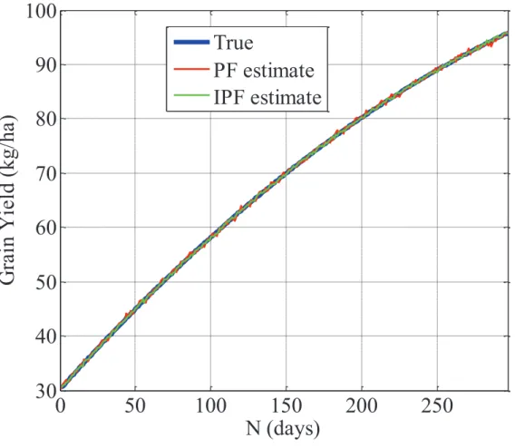
Figure 2: Updated value of grain protein content (kg/ha) versus N (days) using PF and IPF techniques.

(LAI), soil mineral nitrogen supply (SNS) given a single chlorophyll-content measurement ymkperformed at

flowering. Yield and grain protein content at harvest are then estimated from the updated state variables.

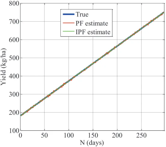
Figures 2, 3 and Table 6 show the estimation of the two states variables Yield and grain protein content

using PF and IPF. The results show the performance of IPF over PF, the efficiency of IPF is due to the

fact it uses the KLD divergence to compute the optimum sampling distribution used to approximate the

posterior density function, which also accounts for the observed data.

Table 6 presents the performance comparison of the state estimation techniques in terms of RMSE and

(23)

0

50

100

150

200

250

100

200

300

400

500

600

700

800 N (days)

Y

ie

ld (kg/

ha

)

True

PF estimate

IPF estimate

Figure 3: Updated value of yield (kg/ha) versus N (Days) using PF and IPF techniques.

Table 6: Comparison of State Estimation Techniques

RMSE Execution times

Technique Yield grain protein content t

PF 1.0761 0.0622 1.11

(24)

4. Conclusions

In this paper, we developed an improved Particle Filter (IPF) for crop model predictions and modeling.

Specifically, two comparative studies are performed. In the first comparative study, we presented a simple

application of the new IPF to a linear dynamic crop model predicting only one state variable, namely winter

wheat biomass and estimating several model parameters. In the second comparative study, we have used

the proposed IPF for updating predictions of complex nonlinear crop models. In this case, the proposed

IPF is applied to a nonlinear model predicting an important winter-wheat quality criterion, grain protein

content and used also to model parameter estimation. In addition to comparing the performances of the

state estimation techniques; Particle Filter (PF), and improved Particle Filter (IPF), the effect of number

of estimated model parameters on the accuracy and convergence of these techniques are also assessed.

The results of both comparative studies show that the IPF provides a significant improvement over the

PF because, unlike the PF which depends on the choice of sampling distribution used to estimate the

posterior distribution, the IPF yields an optimum choice of the sampling distribution, which also accounts

for the observed data. We have investigated the effects of practical challenges on the performances of

Particle Filter (PF), and improved Particle Filter (IPF). The comparative analysis is conducted to study

the effects of two practical challenges (measurement noise, and the number of states and parameters to be

estimated) on the estimation performances of PF, and IPF. To study the effect of measurement noise on

the estimation performances, several measurement noise contributions (e.g., different signal-to-noise ratios)

are considered. Then, the estimation performances of PF and IPF are compared for different noise levels.

Similarly, to investigate the effect of the number of states and parameters to be estimated on the estimation

performances of PF and IPF, the estimation performance is analyzed for different numbers of estimated

states and parameters. The performance of the proposed method is evaluated on a synthetic example in

(25)

Acknowledgement

This work was made possible by Fonds de la Recherche Scientifique (FNRS) grant. The statements made

herein are solely the responsibility of the authors.

References

[1] J. Williams, C. Jones, J. Kiniry, and D. Spanel, “The epic crop growth model,” Trans. ASAE, vol. 32, no. 2, pp. 497–511, 1989.

[2] C. Diepen, J. Wolf, H. Keulen, and C. Rappoldt, “Wofost: a simulation model of crop production,” Soil use and

manage-ment, vol. 5, no. 1, pp. 16–24, 1989.

[3] S. Hansen, H. Jensen, N. Nielsen, and H. Svendsen, NPo-research, A10: DAISY: Soil Plant Atmosphere System Model. Miljøstyrelsen, 1990.

[4] N. Brisson, B. Mary, D. Ripoche, M. Jeuffroy, F. Ruget, B. Nicoullaud, P. Gate, F. Devienne-Barret, R. Antonioletti, C. Durr et al., “Stics: a generic model for the simulation of crops and their water and nitrogen balances. i. theory, and parameterization applied to wheat and corn,” Agronomie, vol. 18, no. 5-6, pp. 311–346, 1998.

[5] B. Basso and J. Ritchie, “Impact of compost, manure and inorganic fertilizer on nitrate leaching and yield for a 6-year maize-alfalfa rotation in michigan,” Agriculture, ecosystems & environment, vol. 108, no. 4, pp. 329–341, 2005.

[6] M. Mansouri, B. Dumont, and M.-F. Destain, “Modeling and prediction of nonlinear environmental system using bayesian methods,” Computers and Electronics in Agriculture, vol. 92, pp. 16–31, 2013.

[7] D. Simon, Optimal State Estimation: Kalman, H∞, and Nonlinear Approaches. John Wiley and Sons, 2006.

[8] M. Grewal and A. Andrews, Kalman Filtering: Theory and Practice using MATLAB. John Wiley and Sons, 2008. [9] M. Mansouri, H. Snoussi, and C. Richard, “A nonlinear estimation for target tracking in wireless sensor networks using

quantized variational filtering,” Proc. 3rd International Conference on Signals, Circuits and Systems, pp. 1–4, 2009. [10] L. Matthies, T. Kanade, and R. Szeliski, “Kalman filter-based algorithms for estimating depth from image sequences,”

International Journal of Computer Vision, vol. 3, no. 3, pp. 209–238, 1989.

[11] R. E. Kalman, “A new approach to linear filtering and prediction problem,” Trans. ASME, Ser. D, J. Basic Eng., vol. 82, pp. 34–45, 1960.

[12] V. Aidala, “Parameter estimation via the kalman filter,” IEEE Trans. on Automatic Control, vol. 22, no. 3, pp. 471–472, 1977.

[13] G. Chen, Q. Xie, and L. Shieh, “Fuzzy kalman filtering,” Journal of Information Science, vol. 109, pp. 197–209, 1998. [14] D. Simon, “Kalman filtering of fuzzy discrete time dynamic systems,” Applied Soft Computing, vol. 3, pp. 191–207, 2003. [15] H. Nounou and M. Nounou, “Multiscale fuzzy kalman filtering,” Engineering Applications of Artificial Intelligence, vol. 19,

(26)

[16] S. Julier and J. Uhlmann, “New extension of the kalman filter to nonlinear systems,” Proceedings of SPIE, vol. 3, no. 1, pp. 182–193, 1997.

[17] L. Ljung, “Asymptotic behavior of the extended kalman filter as a parameter estimator for linear systems,” IEEE Trans.

on Automatic Control, vol. 24, no. 1, pp. 36–50, 1979.

[18] Y. Kim, S. Sul, and M. Park, “Speed sensorless vector control of induction motor using extended kalman filter,” IEEE

Trans. on Industrial Applications, vol. 30, no. 5, pp. 1225–1233, 1994.

[19] E. Wan and R. V. D. Merwe, “The unscented kalman filter for nonlinear estimation,” Adaptive Systems for Signal

Processing, Communications, and Control Symposium, pp. 153–158, 2000.

[20] R. V. D. Merwe and E. Wan, “The square-root unscented kalman filter for state and parameter-estimation,” IEEE

International Conference on Acoustics, Speech, and Signal Processing, vol. 6, pp. 3461–3464, 2001.

[21] S. Sarkka, “On unscented kalman filtering for state estimation of continuous-time nonlinear systems,” IEEE Trans.

Automatic Control, vol. 52, no. 9, pp. 1631–1641, 2007.

[22] Q. Shu, M. W. Kemblowski, and M. McKee, “An application of ensemble kalman filter in integral-balance subsurface modeling,” Stochastic Environmental Research and Risk Assessment, vol. 19, no. 5, pp. 361–374, 2005.

[23] A. H. Elsheikh, C. Pain, F. Fang, J. Gomes, and I. Navon, “Parameter estimation of subsurface flow models using iterative regularized ensemble kalman filter,” Stochastic Environmental Research and Risk Assessment, vol. 27, no. 4, pp. 877–897, 2013.

[24] G. Storvik, “Particle filters for state-space models with the presence of unknown static parameters,” IEEE Trans. on

Signal Processing, vol. 50, no. 2, pp. 281–289, 2002.

[25] A. Doucet and V. Tadi´c, “Parameter estimation in general state-space models using particle methods,” Annals of the

institute of Statistical Mathematics, vol. 55, no. 2, pp. 409–422, 2003.

[26] G. Poyiadjis, A. Doucet, and S. Singh, “Maximum likelihood parameter estimation in general state-space models using particle methods,” in Proc of the American Stat. Assoc, 2005.

[27] F. Gustafsson, F. Gunnarsson, N. Bergman, U. Forssell, J. Jansson, R. Karlsson, and P. Nordlund, “Particle filters for positioning, navigation, and tracking,” Signal Processing, IEEE Transactions on, vol. 50, no. 2, pp. 425–437, 2002. [28] M. Arulampalam, S. Maskell, N. Gordon, and T. Clapp, “A tutorial on particle filters for online nonlinear/non-gaussian

bayesian tracking,” Signal Processing, IEEE Transactions on, vol. 50, no. 2, pp. 174–188, 2002.

[29] A. Doucet and A. Johansen, “A tutorial on particle filtering and smoothing: Fifteen years later,” Handbook of Nonlinear

Filtering, pp. 656–704, 2009.

[30] B. Andrews, T. Yi, and P. Iglesias, “Optimal noise filtering in the chemotactic response of escherichia coli,” PLoS

com-putational biology, vol. 2, no. 11, p. e154, 2006.

[31] N. Yang, W. Tian, Z. Jin, and C. Zhang, “Particle filter for sensor fusion in a land vehicle navigation system,” Measurement

(27)

[32] J. Liu and R. Chen, “Sequential monte carlo methods for dynamic systems,” Journal of the American statistical

associa-tion, pp. 1032–1044, 1998.

[33] J. Kotecha and P. Djuric, “Gaussian particle filtering,” IEEE Trans. on Signal Processing, vol. 51, no. 10, pp. 2592–2601, 2003.

[34] R. Van Der Merwe, A. Doucet, N. De Freitas, and E. Wan, “The unscented particle filter,” Advances in Neural Information

Processing Systems, pp. 584–590, 2001.

[35] J. Vermaak, N. Lawrence, and P. Perez, “Variational inference for visual tracking,” in Conf. Computer Vision and Pattern

Recognition, Jun. 2003.

[36] A. Corduneanu and C. Bishop, “Variational bayesian model selection for mixture distribution,” in Artificial Intelligence

and Statistics, 2001.

[37] C. Varlet-Grancher, R. Bonhomme, M. Chartier, and P. Artis, “Efficience de la conversion de l’´energie solaire par un couvert v´eg´etal,” Acta Oecologica. Oecologia plantarum, 1982.

[38] F. BARET, “Contribution au suivi radiometrique de cultures de cereales,” Ph.D. dissertation, 1986.

[39] M.-H. Jeuffroy and S. Recous, “Azodyn: a simple model simulating the date of nitrogen deficiency for decision support in wheat fertilization,” European journal of Agronomy, vol. 10, no. 2, pp. 129–144, 1999.

[40] J.-M. Meynard, M. Cerf, L. Guichard, M.-H. Jeuffroy, D. Makowski et al., “Which decision support tools for the environ-mental management of nitrogen?” Agronomie-Sciences des Productions Vegetales et de l’Environnement, vol. 22, no. 7-8, pp. 817–830, 2002.