Efficient OLAP Operations For RDF Analytics

HAL Id: hal-01187448

https://hal.inria.fr/hal-01187448

Submitted on 28 Aug 2015

HAL is a multi-disciplinary open access

archive for the deposit and dissemination of

sci-entific research documents, whether they are

pub-lished or not. The documents may come from

teaching and research institutions in France or

L’archive ouverte pluridisciplinaire HAL, est

destinée au dépôt et à la diffusion de documents

scientifiques de niveau recherche, publiés ou non,

émanant des établissements d’enseignement et de

recherche français ou étrangers, des laboratoires

Efficient OLAP Operations For RDF Analytics

Elham Akbari-Azirani, François Goasdoué, Ioana Manolescu, Alexandra

Roatis

To cite this version:

Elham Akbari-Azirani, François Goasdoué, Ioana Manolescu, Alexandra Roatis. Efficient OLAP

Op-erations For RDF Analytics. International Workshop on Data Engineering meets the Semantic Web

(DESWeb), Apr 2015, Seoul, South Korea. �10.1109/ICDEW.2015.7129548�. �hal-01187448�

Efficient OLAP Operations For RDF Analytics

Elham Akbari Azirani

, François Goasdoué

_{, Ioana Manolescu}

, Alexandra Roati¸s

#_{INRIA, France} ∗_{U. Rennes 1, France} ?_{U. Paris-Sud, France}

1_elham@lri.fr 2_fg@irisa.fr 3_{ioana.manolescu@inria.fr} 4_{roatis@lri.fr}

ABSTRACT

RDF is the leading data model for the Semantic Web, and dedi-cated query languages such as SPARQL 1.1, featuring in particu-lar aggregation, allow extracting information from RDF graphs. A framework for analytical processing of RDF data was introduced in [1], where analytical schemas and analytical queries (cubes) are fully re-designed for heterogeneous, semantic-rich RDF graphs. In this novel analytical setting, we consider the following optimiza-tion problem: how to reuse the materialized result of a given RDF analytical query (cube) in order to compute the answer to another cube. We provide view-based rewriting algorithms for these cube transformations, and demonstrate experimentally their practical in-terest.

1.

MOTIVATION AND OUTLINE

Graph-structured, semantics-rich, heterogeneous RDF data needs dedicated warehousing tools [2]. In [1], we have introduced a novel framework for RDF data analytics. At its core lies the concept of analytical schema(AnS, in short), which reflects a view of the data under analysis. Based on an analytical schema, analytical queries (AnQ, in short) can be posed over the data; they are the counterpart of the “cube” queries in the relational data warehouse scenario, but specific to our RDF context. Just like in the traditional relational data warehouse (DW) setting, AnQs can be evaluated either on a materialized AnS instance, or by composing them with the defini-tion of the AnS; the latter is more efficient when AnQ answering only needs a small part of the AnS instance.

In this work, we focus on efficient OLAP operations for the RDF data warehousing context introduced in [1]. More specifically, we consider the question of computing the answer to an AnQ based on the (intermediary) answer of another AnQ, which has been ma-terialized previously. While efficient techniques for such “cube-to-cube” transformations have been widely studied in the relational DW setting, new algorithms are needed in our context, where, un-like the traditional relational DW setting, a fact may have (i) multi-ple values along each dimension and (ii) multimulti-ple measure results. In the sequel, to make this paper self-contained, Sections 2 re-calls the core notions introduced in [1], by borrowing some of its examples; we also recall OLAP operation definitions from that work. Then, we provide novel algorithms for efficiently evaluating such operations on AnQs, briefly discuss related work, and con-clude. An experimental evaluation of our techniques is described in [3].

2.

BACKGROUND: RDF ANALYTICS

RDF analytical schemas and queries. RDF analytical schemas can be seen as lenses through which data is analyzed. An AnS is a labeled directed graph, whose nodes are analysis classes and

Blogger s user1 user2 user3 acquaintedWith . . . Name . . . identifiedBy s o user1 Bill user1 William . . . . City . . . livesIn . . . BlogPost . . . wrotePost . . . Site . . . postedOn . . . hasWordCount. . . Value. . . Age s 28 35 40 . . . hasAge s o user1 28 user2 40 user3 35 . . . .

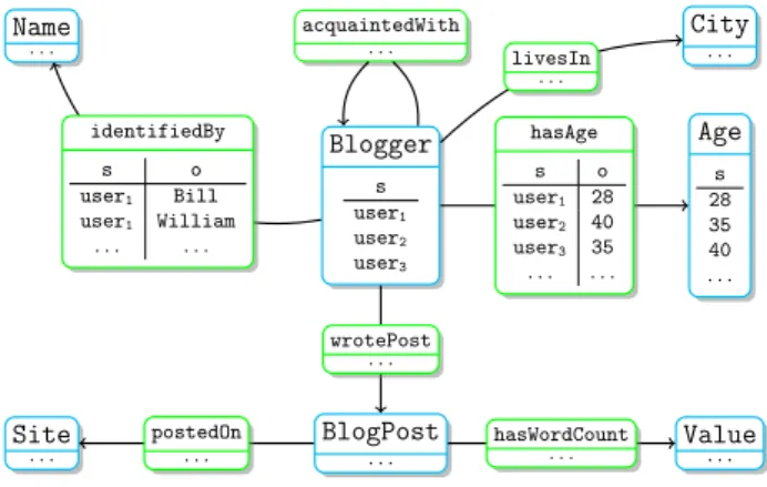
Figure 1: Sample Analytical Schema (AnS).

whose edges are analysis properties, deemed interesting by the data analyst for a specific analysis task. The instance of an AnS is built from the base data; it is an RDF graph itself, heterogeneous and semantic-rich, restructured for the needs of the analysis.

Figure 1 shows a sample AnS for analyzing bloggers and blog posts. An AnS node is defined by an unary query, which, evaluated over an RDF graph, returns a set of URIs. For instance, the node Blogger is defined by a query which (in this example) returns the URIs user1, user2and user3. The interpretation is that the AnS

defines the analysis class Blogger, whose instances are these three users. An AnS edge is defined by a binary query, returning pairs of URIs from the base data. The interpretation is that for each (s, o) URI pair returned by the query defining the analysis property p, the triple s p o holds, i.e., o is a value of the property p of s. Crucial for the ability of AnSs to support analysis of heterogeneous RDF graphs is the fact that AnS nodes and edges are defined by com-pletely independent queries. Thus, for instance, a user may be part of the Blogger instance whether or not the RDF graph comprises value(s) for the analysis properties identifiedBy, livesIn etc. of that user. Further, just like in a regular RDF graph, each blog-ger may have multiple values for a given analysis property. For instance, user1is identified both as William and as Bill.

We consider the conjunctive subset of SPARQL consisting of ba-sic graph pattern(BGP) queries, denoted q(¯x) :- t1, . . . , tα, where

{t1, . . . , tα} are triple patterns. Unless we explicitly specify that a

query has bag semantics, the default semantics we consider is that of set.

The head of q, denoted head(q) is q(¯x), while the body t1, . . . , tα

is denoted body(q). We use letters in italics (possibly with sub-scripts) to denote variables. A rooted BGP query is a query q where each variable is reachable through triples from a distinguished vari-able, denoted root. For instance, the following query is a rooted BGP, whose root is x1:

q(x1, x2, x3) :- x1acquaintedWith x2,

x1identifiedBy y1,

x1wrotePost y2, y2postedOn x3

The query’s graph representation below shows that every node is reachable from the root x1.

x

x

y

y

x

An analytical query consists of two BGP queries homomorphic to theAnS and rooted in the same AnS node, and an aggrega-tionfunction. The first query, called a classifier, specifies the facts and the aggregation dimensions, while the second query, called the measure, returns the values that will be aggregated for each fact. The measure query has bag semantics. Example 1 presents an AnQ over the AnS defined in Figure 1.

EXAMPLE 1. (ANALYTICALQUERY) The query below asks for the number of sites where each blogger posts, classified by the blog-ger’s age and city:

Q :- hc(x, dage, dcity), m(x, vsite), counti

where the classifier and measure queries are defined by: c(x, dage, dcity) :- x rdf:type Blogger,

x hasAge dage, x livesIn dcity

m(x, vsite) :- x rdf:type Blogger,

x wrotePost p, p postedOn vsite

The semantics of an analytical query is:

DEFINITION 1. (ANSWER SET OF ANANALYTICALQUERY) LetI be the instance of an analytical schema with respect to some RDF graph. LetQ :- hc(x, d1, . . . , dn), m(x, v), ⊕i be an

analyt-ical query againstI.

Theanswer set of Q against I, denoted ans(Q, I), is: ans(Q, I) = {hdj1, . . . , d j n, ⊕(qj(I))i | hxj , dj1, . . . , d j

ni ∈ c(I) and qj(I) is the bag

of all valuesv_kjsuch that(xj, vj_k) ∈ m(I)} whereqj_{(I) is a bag containing all measure values v}

correspond-ing toxj

, and the operator⊕ aggregates all members of this bag. If qj(I) is empty, the aggregated measure is undefined, and xjdoes

not contribute to the cube. In the following, for conciseness, we use ans(Q) to denote ans(Q, I), where I is considered the working instance of the analytical schema.

In other words, the AnQ returns each tuple of dimension values from the answer of the classifier query, together with the aggregated result of the measure query for those dimension values. The answer set of an AnQ can thus be represented as a cube of n dimensions, holding in each cube cell the corresponding aggregate measure.

The counterpart of a fact, in this framework, is any value to which the first variable in the classifier, x above, is bound, and that has a non-empty answer for the measure query. In RDF, a re-source may have zero, one or several values for a given property. Accordingly, in our framework, a fact may have multiple values for each measure; in particular, some of these values may be identical, yet they should not be collapsed into one. For instance, if a product is rated by 5 users, one of which rates it ? ? ? while the four others

rate it ?, the number of times each value was recorded is important. This is why we assign bag semantics to qj(I). In all other contexts, we consider BGPs with set semantics; this holds in particular for any classifier query c(x, d1, . . . , dn).

EXAMPLE 2. (ANALYTICAL QUERYANSWER) Consider the AnQ in Example 1, over the AnS in Figure 1. Suppose the classi-fier query’s answer set is:

{huser1, 28, Madridi, huser3, 35, NYi, huser4, 35, NYi}

the measure query is evaluated for each of the three facts, leading to the intermediary results:

xj user1 user3 user4

qj(I) {|hs1i, hs1i, hs2i|} {|hs2i|} {|hs3i|}

where {| · |} denotes the bag constructor. Aggregating the sites among the classification dimensions leads to theAnQ answer:

{h28, Madrid, 3i, h35, NY, 2i}

OLAP for RDF. On-Line Analytical Processing (OLAP) [4] tech-nologies enhance the abilities of data warehouses (so far, mostly relational) to answer multi-dimensional analytical queries. In a re-lational setting, the so-called “OLAP operations” allow computing a cube (the answer to an analytical query) out of another previously materialized cube.

In our data warehouse framework specifically designed for graph-structured, heterogeneous RDF data, a cube corresponds to an AnQ; for instance, the query in Example 1 models a bi-dimensional cube on the warehouse related to our sample AnS in Figure 1. Thus, we model traditional OLAP operations on cubes as AnQ rewrit-ings, or more specifically, rewritings of extended AnQs which we introduce below.

DEFINITION 2. (EXTENDED AnQ) Let S be an AnS, and d1, . . . , dnbe a set of dimensions, each ranging over a non-empty

finite setVi. LetΣ be a total function over {d1, . . . , dn}

associat-ing to eachdi, eitherVior a non-empty subset ofVi. Anextended

analytical query Q is defined by a triple:

Q :- hcΣ(x, d1, . . . , dn), m(x, v), ⊕i

where c is a classifier and m a measure query over S, ⊕ is an aggregation operator, and moreover:

cΣ(x, d1, . . . , dn) =

S

(χ1,...,χn)∈Σ(d1) × ...×Σ(dn)c(x, χ1, . . . , χn)

In the above, the extended classifier cΣ(x, d1, . . . , dn) is the set

of all possible classifiers obtained by replacing each dimension variablediwith a value fromΣ(di). We introduce Σ to constrain

some classifier dimensions, i.e., to restrict the classifier result. The semantics of an extended analytical queryis derived from the se-mantics of a standard AnQ (Definition 1) by replacing the tuples from c(I) with tuples from cΣ(I). Thus, an extended analytical

query can be seen as a union of a set of standard AnQs, one for each combination of values in Σ(d1), . . . , Σ(dn). Conversely, an

analytical query corresponds to an extended analytical query where Σ only contains pairs of the form (di, Vi).

ASLICEoperation binds an aggregation dimension to a single value. Given an extended query Q :- hcΣ(x, d1, . . . , dn), m(x, v),

⊕i, aSLICEoperation over a dimension diwith value vireturns the

extended query QSLICE:- hcΣ0(x, d1, . . . , dn), m(x, v), ⊕i, where

Σ0= (Σ \ {(di, Σ(di))}) ∪ {(di, {vi})}.

Similarly, a DICE operation constrains several aggregation di-mensions to values from specific sets. ADICEon Q over dimen-sions {di1, . . . , dik} and corresponding sets of values {Si1, . . . ,

Si_k}, returns the query QDICE:- hcΣ0(x, d1, . . . , dn), m(x, v), ⊕i,

where Σ0= (Σ \Sik

j=i1{(dj, Σ(dj))}) ∪

Sik

j=i1{(dj, Sj)}.

ADRILL-OUToperation on Q over dimensions {di1, . . . , dik}

corresponds to removing these dimensions from the classifier. It leads to a new query QDRILL-OUThaving the classifier cΣ0(x, d_j1, . . . , d_j

n−k), where dj1, . . . , djn−k ∈ {d1, . . . , dn} \ {di1, . . . , dik} and Σ 0 = (Σ \Sik j=i1{(dj, Σ(dj))}).

Finally, a DRILL-IN operation on Q over dimensions {dn+1, . . . , dn+k} which all appear in the classifier’s body and

have value sets {Vn+1, . . . , Vn+k} corresponds to adding these

di-mensions to the head of the classifier. It produces a new query QDRILL-INhaving the classifier cΣ0(x, d1, . . . , dn, dn+1, . . . , dn+k),

where the dimensions dn+1, . . . , dn+k 6∈ {d1, . . . , dn},

Σ0= (Σ ∪Si_k

j=i1{(dj, Vj)}).

These operations are illustrated in the following example. EXAMPLE 3. (OLAP OPERATIONS) Let Q be the extended query

corresponding to the query-cube defined in Example 1, that is:Q :- hc(x, dage, dcity),

m(x, vsite), counti, Σ = {(dage, Vage), (dcity, Vcity)} (the

clas-sifier and measure are as in Example 1).

ASLICEoperation on thedagedimension with value 35 replaces

the extended classifier ofQ with cΣ0(x, dage, dcity) = {c(x, 35, dcity)}

whereΣ0= Σ \ {(dage, Vage)} ∪ {(dage, {35})}.

ADICEoperation on bothdageanddcitydimensions with

val-ues{28} for dageand{Madrid, Kyoto} for dcityreplaces the

ex-tended classifier ofQ with cΣ0(x, dage, dcity) = {c(x, 28, Madrid),

c(x, 28, Kyoto)} where Σ0= {(dage, {28}), (dcity, {Madrid, Kyoto})}.

ADRILL-OUTon thedagedimension producesQDRILL-OUT:-hc

0

Σ0(x, dcity),

m(x, vsite), counti with Σ0 = {(dcity, Vcity)} and body(c0) ≡

body(c).

Finally, aDRILL-INon thedagedimension applied to the query

QDRILL-OUTabove producesQ, the query of Example 1.

3.

OPTIMIZED OLAP OPERATIONS

The above OLAP operations lead to new queries, whose answers can be computed based on the AnS instance. The focus of the present work is on answering such queries by using the materialized results of the initial AnQ, and (only when that input is insufficient) more data, such as intermediary results generated while computing AnQ results, or (a small part of) the AnS instance. These results are often significantly smaller than the full instance, hence obtain-ing the answer to the new query based on them is likely faster than computing it from the instance. Figure 2 provides a sketch of the problem.

In the following, all relational algebra operators are assumed to have bag semantics.

Given an analytical query Q whose measure query (with bag se-mantics) is m, we denote by ¯m the set-semantics query whose body is the same as the one of m and whose head comprises all the vari-ables ofm’s body. Obviously, there is a bijection between the bag result of m and the set result of ¯m. Using ¯m, we define next the intermediary answer of an AnQ.

DEFINITION 3. (INTERMEDIARY QUERY OF ANANQ) Let Q

:-Analytical query Q

Analytical query QT

apply OLAP transf. T (described in Section 2)

Answer to Q – ans(Q) d1 d2 . . . dn v

Partial result – pres(Q) x d1 d2 . . . dn k m evaluate c and m of Q on I aggregate column m Answer to QT d1 d2 . . . dm v evaluate QTon I

How to simulate the transf. T by rewriting QTusing pres(Q)

or ans(Q) (and I if necessary).

Figure 2: Problem statement.

hc, m, ⊕i be an AnQ. The intermediary query of Q, denoted int(Q), is:

int(Q) = c(x, d1, . . . , dn) ./xm(x, v)¯

It is easy to see that int(Q) holds all the information needed in order to compute bothc and m; it holds more information than the results of c and m, given that it preserves all the different embed-dings of the (bag-semantics) m query in the data. Clearly, evalu-ating int is at least as expensive as evaluevalu-ating Q itself; while int is conceptually useful, we do not need to evaluate it or store its results.

Instead, we propose to evaluate (possibly as part of the effort for evaluating Q), store and reuse a more compact result, defined as follows. For a given query Q whose measure (with bag semantics) is m, we term extended measure result over an instance I, denoted mk(I), the set defined by:

{(newk(), t) | t ∈ m(I)}

where newk() is a key-creating function returning a distinct value at each call. A very simple implementation of newk(), which we will use for illustration, returns successively 1, 2, 3 etc. We assign a key to each tuple in the measure so that multiple identical values of a given measure for a given fact would not be erroneously collapsed into one. For instance, if

m(I) = {|(x1, m1), (x1, m1), (x1, m2), (x2, m3)|},

then

mk_{(I) = {(1, x}

1, m1), (2, x1, m1), (3, x1, m2), (4, x2, m3)}.

DEFINITION 4. (PARTIAL RESULT OF ANANQ) Let Q :- hc, m, ⊕i be an AnQ. The partial result of Q on an instance I, denoted pres(Q, I) is:

pres(Q, I) = c(I) ./xmk(I)

One can see pres(Q, I) as the input to the last aggregation per-formed in order to answer the AnQ, augmented with a key. In the

following, we use pres(Q) to denote pres(Q, I) for the working instance of the AnS.

Problem Statement : (ANSWERINGAnQS USING THE MATE

-RIALIZED RESULTS OF OTHER AnQS) Let Q, QT be AnQs

such that applying the OLAP transformation T on Q leads to QT.

The problem of answering QT using the materialized result of Q

consists of finding: (i) an equivalent rewriting of QT based on

pres(Q) or ans(Q), if one exists; (ii) an equivalent rewriting of QTbased on pres(Q) and the AnS instance, otherwise.

Importantly, the following holds:

πx,d1,...,dn,v(int(Q)(I)) = πx,d1,...,dn,v(pres(Q, I)) (1)

Q ≡ γd1,...,dn,⊕(v)(πx,d1,...,dn,v(int(Q))) (2)

ans(Q)(I) = γd1,...,dn,⊕(v)(πx,d1,...,dn,v(pres(Q, I))) (3)

Equation (1) directly follows from the definition of pres. Equa-tion (2) will be exploited to establish the correctness of some of our techniques. Equation (3) above is the one on which our rewriting-based AnQ answering technique is rewriting-based.

3.1

Slice and Dice

In the case ofSLICEandDICEoperations, the data cube transfor-mation is made simply by row selection over the materialized final results of an AnQ.

EXAMPLE 4. (DICE) The query Q asks for the average number of words in blog posts, for each blogger’s age and residential city.

Q :- hc(x, dage, dcity), m(x, vwords), averagei

c(x, dage, dcity) :- x rdf:type Blogger,

x hasAge dage, x livesIn dcity

m(x, vwords) :- x rdf:type Blogger,

x wrotePost p, p hasWordCount vwords

Suppose the answer ofc over I is

{huser1, 28, Madridi, huser3, 35, NYi, huser4, 28, Madridi}

and the answer ofm over I is

{|huser1, 100i, huser1, 120i, huser3, 570i, huser4, 410i|}

Joining the answers ofc and m in such a query results in: {|huser1, 28, Madrid, 100i, huser1, 28, Madrid, 120i,

huser3, 35, NY, 570i, huser4, 28, Madrid, 410i|}

The final answer toQ after aggregation is: {h28, Madrid, 210i, h35, NY, 570i}

The queryQDICEis the result of aDICEoperation onQ,

restrict-ing thedageto values between20 and 30. QDICEdiffers fromQ only

by its classifier which can be written ascΣ0(x, dage, dcity) where

Σ0= Σ \ {(dage, Vage)} ∪ {(dage, {dage}20≤dage≤30)}.

ApplyingDICEon the answer toQ above yields the result: {h28, Madrid, 210i}

Now, we calculate the answer toQDICE. The result of the classifier

querycΣ0, obtained by applying a selection on thedagedimension

is:

{huser1, 28, Madridi, huser4, 28, Madridi}

Evaluatingm and joining its result with the above set yields: {|huser1, 28, Madrid, 100i, huser1, 28, Madrid, 120i,

huser4, 28, Madrid, 410i|}

The final answer toQDICEafter aggregation is:

{h28, Madrid, 210i}

DICEapplied over the answer ofQ yields the answer of QDICE.

DEFINITION 5. (SELECTION) Let dice be a dice operation on analytical queries. Let Σ0 be the function introduced in Defini-tion 2. We define aselection σdiceas a function on the space of

analytical query answersans(Q) where:

σdice(ans(Q)) = {hd1, . . . , dn, vi|hd1, . . . , dn, vi ∈ ans(Q)

∧ ∀i ∈ {1, . . . , n} di∈ Σ0(di)}

PROPOSITION 1. Let Q :- hcΣ(x, d1, . . . , dn), m(x, v), ⊕i and

QDICE:-hc

0

Σ0(x, d1, . . . , dn), m0(x, v), ⊕i be two analytical queries

such that queryQDICE= dice(Q). Then σdice(ans(Q)) = ans(QDICE).

The proofs for all our results can be found in [3].

3.2

Drill-Out

Unlike the relational DW setting, in our RDF warehousing frame-work the result of a drill-out operation (that is, the answer to QDRILL-OUT)

cannot be correctly computed directly from the answer to the orig-inal query Q, and here is why. Each tuple in ans(Q) binds a set of dimension values to an aggregated measure. In fact, each such tuple represents a set of facts having the same dimension values. Projecting a dimension out will make some of these sets merge into one another, requiring a new aggregation of the measure values. Computing this new aggregated measure from the ones in ans(Q) will require considering whether the aggregation function has the distributiveproperty, i.e., whether ⊕(a, ⊕(b, c)) = ⊕(⊕(a, b), c). 1. Distributive aggregation function, e.g. sum. In this case, the new aggregated measure value could be computed from ans(Q) if the sets of facts aggregated in each tuple of ans(Q) were mutually exclusive. This is not the case in our setting where each fact can have several values along the same di-mension. Thus, aggregating the already aggregated measure values will lead to erroneously consider some facts more than once; avoiding this requires being able to trace the measure results back to the facts they correspond to.

2. Non-distributive aggregation function, e.g., avg. For such functions, the new aggregated measure must be computed from scratch.

Based on the above discussion, we propose Algorithm 1 to com-pute the answer to QDRILL-OUT, using the partial result of Q, denoted

pres(Q) above, which we assume has been materialized and stored as part of the evaluation of the original query Q. This deduplication (δ) step is needed, since some facts may have been repeated in T for being multivalued along di. The aggregation function ⊕ is applied

to the measure column of the resulting relation T , using γ, group-ing the tuples along the dimensions d1, . . . , di−1, di+1, . . . , dn.

Algorithm 1DRILL-OUTcube transformation 1: Input: pres(Q), di

2: T ← Πroot,d1,...,di−1,di+1,...,dn,k,v(pres(Q))

3: T ← δ(T )

4: T ← γd1,...,di−1,di+1,...,dn,⊕(v)(T )

5: return T

PROPOSITION 2. Let Q be an AnQ and QDRILL-OUTbe the AnQ

obtained fromQ by drilling out along the dimension di.

Algo-rithm 1 applied onpres(Q) and dicomputesans(QDRILL-OUT).

Example 5 illustrates Algorithm 1, and also shows how relying only on ans(Q) may introduce errors.

EXAMPLE 5. (DRILL-OUT) Consider an analytical query Q such that its classifierc1, measurem and intermediary answer pres(Q)

have the results shown below.

c1 root d1 . . . dn−1 dn x a1 . . . an−1 an x a1 . . . an−1 bn y a1 . . . an−1 bn m k root v 1 x m1 2 y m2 pres(Q) root d1 . . . dn−1 dn k v x a1 . . . an−1 an 1 m1 x a1 . . . an−1 bn 1 m1 y a1 . . . an−1 bn 2 m2 (i)

LetQDRILL-OUTbe the result of aDRILL-OUToperation onQ

elim-inating dimensiondn. The measure ofQDRILL-OUTis stillm, while

its classifierc2has the answer shown next:

c2

root d1 . . . dn−1

x a1 . . . an−1

y a1 . . . an−1

Note thatc2returns only one row forx, because it has one value

for the dimension vectorhd1, . . . , dn−1i. pres(QDRILL-OUT) yields:

root d1 . . . dn−1 k v

x a1 . . . an−1 1 m1

y a1 . . . an−1 2 m2

Applying aggregation over the above table leads to:

d1 . . . dn−1 v

a1 . . . an−1 ⊕({m1, m2})

(ii)

Algorithm 1 on the input(i), first projects out dn. TableT after

projecting outdnfrompres(Q) is:

root d1 . . . dn−1 k v

x a1 . . . an−1 1 m1

x a1 . . . an−1 1 m1

y a1 . . . an−1 2 m2

After eliminating duplicates (δ(T )), grouping and aggregation, we obtain:

d1 . . . dn−1 v

a1 . . . an−1 ⊕({m1, m2}) (iii)

The output of Algorithm 1 above, denoted(iii), is the same as (ii), showing that our algorithm answers QDRILL-OUTcorrectly using

the intermediary answer ofQ.

Next we examine what would happen if an algorithm took the answer ofQ as input. First, we compute ans(Q), by aggregating the measures along the dimensions from the intermediary result de-picted in(i):

ans(Q)

d1 . . . dn−1 dn v

a1 . . . an−1 an ⊕({m1})

a1 . . . an−1 bn ⊕({m1, m2})

Next we project outdnfromans(Q):

d1 . . . dn−1 v

a1 . . . an−1 ⊕({m1})

a1 . . . an−1 ⊕({m1, m2})

and aggregate, assuming that⊕ is distributive. d1 . . . dn−1 v

a1 . . . an−1 ⊕({m1, m1, m2})

(iv)

Observe that(iv) is different from (ii). More specifically, the mea-sure value corresponding to the multi-valued entityx has been con-sideredtwice in the aggregated measure value of (iv).

3.3

Drill-In

The drill-in operation increases the level of detail in a cube by adding a new dimension. In general, this additional information is not present in the answer of the original query. Hence, answering the new query requires extra information.

Algorithm 2DRILL-INcube transformation 1: Input: pres(Q, I), c, dn+1

2: build qQ

aux(dvars, dn+1) :- body . as per Definition 6

3: T ← pres(Q, I)1dvarsqauxQ (I)

4: T ← γd1,...,dn,dn+1,⊕(v)(T )

5: return T

Algorithm 2 uses the partial result of Q, denoted pres(Q), and consults the materialized AnS instance to obtain the missing infor-mation necessary to answer QDRILL-IN. We retrieve this information

through an auxiliary query defined as follows.

DEFINITION 6. (AUXILIARY DRILL-IN QUERY) Let Q :- hc(x, d1, . . . , dn),

m(x, v), ⊕i be an AnQ and dn+1a non-distinguished variable in

c. The auxiliaryDRILL-INquery ofQ over dn+1is a conjunctive

queryqauxQ (dvars, dn+1) :- bodyaux, where

• each triple t ∈ body(c) containing the variable dn+1is also

I

s p o

website1 hasUrl URL1

website1 supportsBrowser firefox

website2 hasUrl URL2

website2 supportsBrowser chrome video1 postedOn website1 video1 postedOn website2

video1 type Video

video1 viewNum n pres(Q) x d2 k v video1 URL1 1 n video1 URL2 2 n ans(Q) d2 v URL1 n URL2 n pres(QDRILL-IN) x d2 d3 k v

video1 URL1 firefox 1 n video1 URL2 chrome 2 n ans(QDRILL-IN)

d2 d3 v

URL1 firefox n URL2 chrome n

x d2 d3 k v

video1 URL1 firefox 1 n video1 URL2 chrome 1 n

Figure 3:DRILL-INexample.

• for each triple tauxinbodyauxandt in the body of c such

thatt and tauxshare a non-distinguished variable ofc, the

triplet also belongs to bodyaux;

• each variable in bodyauxthat is distinguished inc is a

dis-tinguished variableqQ aux.

The auxiliary query qauxQ comprises all triples from Q’s

classi-fier having the dimension dn+1; to these, it adds all the classifier

triples sharing a non-distinguished (existential) variable with the former; then all the classifier triples sharing an existential variable with a triple previously added to bodyauxetc. This process stops

when there are no more existential variables to consider. The vari-ables distinguished in c, together with the new dimension dn+1, are

distinguished in qQaux.

PROPOSITION 3. Let Q :- hc, m, ⊕i be an analytical query and dn+1be a non-distinguished variable inc. Let QDRILL-INbe the

an-alytical query obtained fromQ by drilling in along the dimension dn+1, andI be an instance. Algorithm 2 applied on pres(Q, I), c

anddn+1computesans(QDRILL-IN)(I).

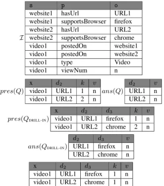
EXAMPLE 6. (DRILL-IN REWRITING) Let Q :- hc, m, sumi be the following AnQ:

c(x, d2) :- x rdf:type Video, x uploadedOn d1,

d1hasUrl d2, d1supportsBrowser d3

m(x, v) :- x rdf:type Video, x viewNum v

QDRILL-INis the result of a DRILL-INthat adds the dimensiond3,

having the classifier queryc0(x, d2, d3).

Figure 3 shows the materialized analytical schema instance, the partial and final answer toQ, and the partial and final answer

toQDRILL-IN. Now, let us see how to answerQDRILL-INusing

Algo-rithm 2. We have: qQ

aux(x, d2, d3) :- x postedOn d1, d1hasUrl d2,

d1supportsBrowser d3

Based onI, the answer to qQ auxis:

x d2 d3

video1 URL1 firefox video1 URL2 chrome

Joining the above withpres(Q) yields the last table in Figure 3, which after aggregation yields the result ofQDRILL-IN.

4.

RELATED WORK

Previous RDF data management research focused on efficient stores, query processing, view selection etc. BGP query answering techniques have been studied intensively, e.g., [5, 6], and some are deployed in commercial systems such as Oracle 11g’s “Semantic Graph” extension. Our optimizations can be deployed on top of any RDF data management platform, to extend it with optimized analytic capabilities.

The techniques we presented can be seen as a particular case of view-based rewriting [7], where partial AnQ results are used as a materialized view. Novel algorithms were required due to the novel AnQ language we introduced in [1].

SPARQL 1.1 [8] features SQL-style grouping and aggregation, less expressive than our AnQs, as our measure queries allow more flexibility than SPARQL. Thus, the OLAP operation optimizations we presented can also apply to the more restricted SPARQL ana-lytical context.

OLAP has been thoroughly studied in a relational setting, where it is at the basis of a successful industry; in particular, OLAP op-eration evaluation by reusing previous cube results is well-known. The heterogeneity of RDF, which in turn justified our novel RDF analytics framework [1], leads to the need for the novel algorithms we described here, which are specific to this setting.

5.

CONCLUSION

Our work focused on optimizing the OLAP transformations in the RDF data warehousing framework we introduced in [1], by us-ing view-based rewritus-ing techniques. To this end, for each OLAP operation, we introduced an algorithm that answers a transformed query based on the final or on an intermediary result of the original analytical query. We formally prove the correctness of our tech-niques, and describe experiments performed with our algorithms, in our technical report [3].

6.

REFERENCES

[1] D. Colazzo, F. Goasdoué, I. Manolescu, and A. Roatis, “RDF analytics: lenses over semantic graphs,” in WWW, 2014. [2] S. Spaccapietra, E. Zimányi, and I. Song, Eds., Journal on

Data Semantics XIII, ser. LNCS, vol. 5530. Springer, 2009. [3] E. Akbari, F. Goasdoué, I. Manolescu, and A. Roati¸s,

“Efficient OLAP operations for RDF analytics,” INRIA Research Rep. RR-8668, Jan. 2015.

[4] “OLAP Council White Paper,” http://www.olapcouncil.org/research/ resrchly.htm.

[5] F. Goasdoué, I. Manolescu, and A. Roati¸s, “Efficient query answering against dynamic RDF databases,” in EDBT, 2013. [6] J. Pérez, M. Arenas, and C. Gutierrez, “nSPARQL: A

navigational language for RDF,” J. Web Sem., vol. 8, no. 4, 2010.

[7] A. Y. Halevy, “Answering queries using views: A survey,” VLDB J., vol. 10, no. 4, 2001.

[8] W3C, “SPARQL 1.1 query language,”