Spatial Evolution of the Thickness Variations over a CFRP Laminated Structure

HAL Id: hal-01841955

https://hal.archives-ouvertes.fr/hal-01841955

HAL is a multi-disciplinary open access archive for the deposit and dissemination of sci-entific research documents, whether they are pub-lished or not. The documents may come from teaching and research institutions in France or abroad, or from public or private research centers.

L’archive ouverte pluridisciplinaire HAL, est destinée au dépôt et à la diffusion de documents scientifiques de niveau recherche, publiés ou non, émanant des établissements d’enseignement et de recherche français ou étrangers, des laboratoires publics ou privés.

Spatial Evolution of the Thickness Variations over a

CFRP Laminated Structure

Yves Davila, Laurent Crouzeix, Bernard Douchin, Francis Collombet,

Yves-Henri Grunevald

To cite this version:

Yves Davila, Laurent Crouzeix, Bernard Douchin, Francis Collombet, Yves-Henri Grunevald. Spa-tial Evolution of the Thickness Variations over a CFRP Laminated Structure. Applied Composite Materials, Springer Verlag (Germany), 2017, 24 (5), pp.1201 - 1215. �10.1007/s10443-016-9573-5�. �hal-01841955�

Spatial evolution of the thickness variations over a CFRP laminated

structure

Yves Davilaa§_{, Laurent Crouzeix}a_{, Bernard Douchin}a_{, Francis Collombet}a_{, Yves-Henri Grunevald}b a_{: Université de Toulouse, INSA, UPS, Mines d’Albi, ISAE, ICA (Institut Clément Ader), 3 rue Caroline} Aigle, F-31400 Toulouse.

b_{: Composites Expertise & Solutions, 4 rue Georges Vallerey, F-31320 Castanet Tolosan.} § _{Corresponding author’s email: [email protected]}

Keywords: Variability; Composite structure; Thickness; Discrete Fourier transform; Finite element analysis (FEA); Autoclave; Unidirectional prepreg

Davila, Y., Crouzeix, L., Douchin, B., Collombet, F., Grunevald, Y.-H.: Spatial evolution of the thickness variations over a CFRP laminated structure. Appl. Compos. Mater. 24, 1201–1215 (2017).

https://doi.org/10.1007/s10443-016-9573-5

Abstract

Ply thickness is one of the main drivers of the structural performance of a composite part. For stress analysis calculations (e.g., finite element analysis), composite plies are commonly considered to have a constant thickness compared to the reality (coefficients of variation up to 9 % of the mean ply thickness). Unless this variability is taken into account reliable property predictions cannot be made. A modelling approach of such variations is proposed using parameters obtained from a 16-ply quasi-isotropic CFRP plate cured in an autoclave. A discrete Fourier transform algorithm is used to analyse the frequency response of the observed ply and plate thickness profiles. The model inputs, obtained by a mathematical representation of the ply thickness profiles, permit the generation of a representative stratification considering the spatial continuity of the thickness variations that are in good agreement with the real ply profiles spread over the composite part. A residual deformation FE model of the composite plate is used to illustrate the feasibility of the approach.

1.

Introduction

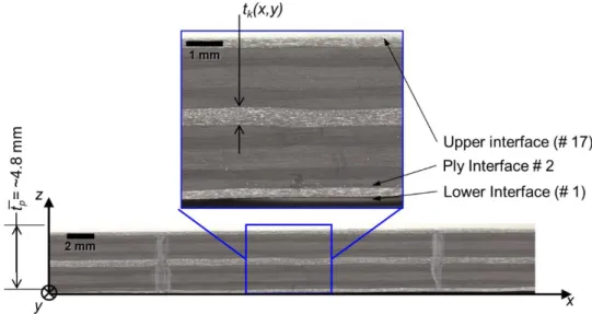
compared to classic engineering materials, such as metals. Such variabilities can be traced from the mesoscopic through structural scales. However the great number of variables make of this task a great challenge [1]. One of these sources of variability is the structure thickness. For design purposes, the thickness of a composite structure is given by the sum of the ply thicknesses forming the laminate, or alternatively, the ply thickness is obtained by dividing the total structure thickness by the number of plies contained in the stratification. The thickness of the structure is considered constant and equal for all plies, provided that there is no change of geometry in the cross-section of the composite structure [2]. In reality, each ply in the stratification does not present a constant thickness mainly due to manufacturing conditions and particularly the resin flow effect before polymerisation in autoclave. Figure 1 exhibits, for different scales, the variations pf ply thickness across a 16-ply unidirectional carbon/epoxy laminate.

Figure 1. Micrograph showing the ply thickness variations tk(x,y) spread over a layered composite plate

(16-ply HexPly® M10.1/38%/UD300/CHS) of approximately 4.8 mm thick t̅p.

The effects of the ply thickness variations have been studied in the literature as localized defects due to manufacturing conditions, in the form of wrinkles and warpings [2,3], and on singular zones such as L-shaped stringers [5]. Conversely, there are few publications that address the representation of thickness variations spread over a laminated structure. Collombet et al. [6] reported a mean ply thickness of 0.26 mm with a standard deviation of 0.002 mm, with extreme values between 0.26 mm and 0.27 mm, in a 28-ply M21/T700 carbon/epoxy laminate. However, the determination of the ply thickness was performed through the measurement of the laminate thickness. A further inspection of the cross section

of the specimens revealed that the ply thicknesses deviated up to 21 % from the mean ply thickness, with extreme values of 0.25 mm and 0.31 mm [6]

It is well-known that the composite structure cannot be dissociated from its manufacturing conditions. The volume fractions of constituent materials (fibre and matrix) as well as porosities are directly linked to the stratification of the composite, the nature of the raw materials and the curing cycle [6,7]. These changes in the volume fraction can be a source of warpages for thin laminates (global on the scale of the plate and “local” on the scale of the plies). Daniel et al. [8,9] have studied the effects of the fibre waviness on thick unidirectional stratifications (up to 150 plies) generated by local and periodic perturbations in the stratification. The proposed method calls for a modification in the compliance matrix by adding an out-of-plane component to the fibre orientation. Nonetheless the problem is treated as a local effect related to defects present in the material.

A classic computational analysis of a composite structure is done by employing a unique value of ply thickness for all the elements [10,11]. Conversely in the literature, no methodology was found that accounts for the local changes spread over the composite structure applied to multidirectional laminates fabricated with UD prepregs.

The aim of this study is to include the “continuous” ply thickness variation in a finite element (FE) model considering actual variations of thicknesses in the composite laminate. This is essential in order to make more realistic property predictions.

To retrieve the required information needed by the numerical model, the cross-section of a 16-ply composite plate is analysed to obtain the real profiles of the ply thicknesses spread over the plate. A discrete Fourier transform (DFT) of the measured ply thickness profiles provides the model parameters. These parameters are analysed to be then introduced into a mathematical model to produce a digital representation of the ply variations. This mathematical model can be modified by the introduction of random parameters that modify the shape of digital lay-ups for their use in different simulations. The set of digital lay-ups containing the variations of the plate and ply thicknesses is then used to calculate the material property of the composite ply that will be afterwards introduced into a FE model.

2.

Material

A set of composite plates was fabricated using a unidirectional carbon/epoxy prepreg HexPly® M10.1/38%/UD300/CHS supplied by Hexcel Composites. The dimensions of the manufactured plates are 600 mm long and 300 mm wide. The 16-ply stratification was chosen to be quasi-isotropic with the lay-up sequence [90/-45/0/(+45)2/0/-45/90]s. The plates were cured in autoclave using the recommended cure cycle adding a consolidation dwell at 90 °C for 15 minutes. The cure dwell was maintained at 120 °C for 60 minutes. The heating and cooling rates were set to 2 °C min-1_{. The consolidation pressure at the} first dwell and the curing pressure in the second dwell were 2 and 5 bar respectively.

3.

Thickness measurements

3.1. Overall plate thickness

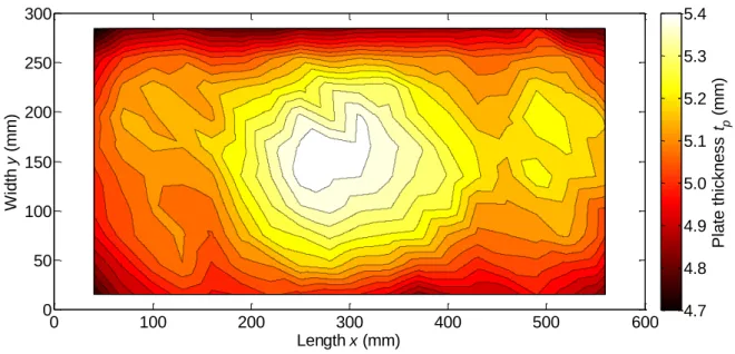
The overall thickness of the cured plates is measured using a 3D coordinate-measuring machine (CMM) with a mechanical probe and a resolution of 0.01mm. With a mesh size of 30 x 30 mm, between 190 and 220 measurement points are needed to cover the complete plate. Figure 2 illustrates the thickness mapping reconstructed using the measurements. The 5.45 mm maximum thickness value is located at the centre of the plate while the 4.68 mm minimum thickness value is closer to the edges and corners of the plate. The difference between the maximum and minimum values is 0.77 mm. This difference is approximately 2.5 times the thickness of the cured ply, considering a nominal ply thickness of 0.32 mm. Olave [13] reported variations in the order of 0.80 to 1.00 mm for a plate of 300 x 300 mm dimensions fabricated with a HexPly® _{M10.1/T700 2/2 twill woven textile. Notice that both types of plates, the ones} studied by Olave and the ones presented here, were fabricated under similar manufacturing conditions.

Figure 2. Example of measured tp(x,y) thickness distribution of the HexPly® M10.1/38%/UD300/CHS plate.

3.2. Ply thickness profile

To determine the profiles of the ply thickness, a 45 x 45 mm specimen was removed from one of the manufactured plates. It exhibits a 4.66 mm mean plate thickness with 4.84 mm and 4.53 mm, maximum and minimum values respectively. Being a section of the composite plate, the difference between the maximum and minimum values is 0.31 mm (compared to 0.77 mm for the complete composite plate).

The specimen was placed on mounting resin to prepare its cross-section for micrographic inspection. A series of micrographs of the cross-section was taken with a Dino-Lite® _{optical microscope} with a 161 pixels/mm resolution. For determining the spatial evolution of the ply thicknesses, the micrographs were assembled into a single image containing the full length of the specimen to avoid duplicated points on the ply interfaces, as each micrograph only covers approximately 7 mm (of the 45 mm) of the length of the specimen. An automatic determination of the ply interfaces by image analysis is preferred. However, the low contrast and fuzziness at the ply interfaces makes it difficult to analyse the images with good precision. Hence, the plies were then delimited by manually selecting the points along the ply interface. A grid on top of the image provides a reference in order to have a rough control of the number of points and their spacing. Approximately 220 points were selected for each interface. The

Length x (mm) W id th y ( m m ) 0 100 200 300 400 500 600 0 50 100 150 200 250 300 P la te t h ickn e ss t p ( m m ) 4.7 4.8 4.9 5.0 5.1 5.2 5.3 5.4

selected points were interpolated into a regular mesh consisting of 1024 points along the x-axis. Figure 3 shows the ply interface selection for the interfaces # 2, # 3 and # 4 (delimiting plies # 2 and # 3).

Figure 3. Profiles for the interfaces # 2 # 3 and # 4 delimiting plies # 2 and # 3 with the cross markings showing the selected points along the ply interface, and the continuous lines showing the interpolated

interfaces.

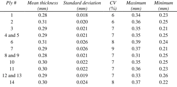
A summary of the basic statistical measurements for all the plies and the composite plate thicknesses is shown in Table 1. Due to the lay-up sequence, the pairs of plies # 4/# 5, # 8/# 9 and # 12/# 13 share the same orientation, thus their interfaces were not discernible and they were counted as single plies. Nonetheless, for the present analysis their mean value, as well as the extreme values, are divided by 2 and their standard deviations are obtained thus by √𝜎 ² 2⁄ .

Table 1. Statistical summary for the ply and plate thickness measurements.

Ply # Mean thickness

(mm) Standard deviation (mm) CV (%) Maximum (mm) Minimum (mm) 1 0.28 0.018 6 0.34 0.23 2 0.31 0.020 6 0.36 0.25 3 0.29 0.021 7 0.35 0.21 4 and 5 0.29 0.021 7 0.35 0.25 6 0.31 0.026 8 0.39 0.24 7 0.29 0.026 9 0.37 0.21 8 and 9 0.28 0.021 7 0.31 0.25 10 0.30 0.022 7 0.35 0.25 11 0.30 0.022 7 0.36 0.23 12 and 13 0.29 0.019 7 0.33 0.26 14 0.30 0.024 8 0.37 0.22 0,6 0,7 0,8 0,9 1,0 1,1 1,2 1,3 1,4 1,5 0 5 10 15 20 25 30 35 40 45 Int erf ac e p os iti on z ( m m ) Width (mm) Ply # 1 Ply # 2 Ply # 3 Ply # 4 Interface # 3 Interface # 4 Interface # 2

15 0.29 0.021 7 0.34 0.21

16 0.27 0.021 8 0.33 0.23

Plate 4.66 0.090 2 4.86 4.49

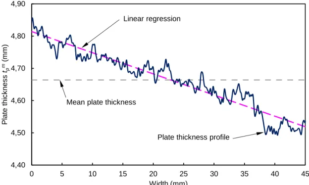
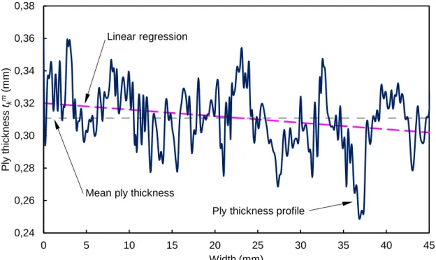
Figure 4 and 5 show the measured thickness profile, mean value and linear regression for the composite plate and the # 2 ply respectively. The coefficient of variation (CV) of the composite plate is 2 %. In comparison, the CVs of the composite plies fall within the range of 4 % to 9 %. It should be noted that the CV of the plate comprises a large difference in thickness at both ends of the specimen length (0.31 mm), shown by the linear regression in Figure 4. While for the ply thickness profile, using the case of ply #2 as example (cf. Figure 5), the CV comprises a difference at both ends of the specimen of 0.02 mm and, more importantly, large variations up to ± 29 % of the mean ply thickness (cf. Table 1).

Figure 4. Profile of the measured plate thickness and the least squares linear fit (dashed line) and the mean thickness (dashed horizontal line).

4,40 4,50 4,60 4,70 4,80 4,90 0 5 10 15 20 25 30 35 40 45 P late thi c k ne s s tp m (m m ) Width (mm)

Plate thickness profile Linear regression

Figure 5. Thickness profile for the ply # 2 and the least squares linear fit (dashed line) and the mean thickness (dashed horizontal line).

It is noteworthy that the difference between the slope of the linear regression (m) of the ply profiles and the mean thickness (zero slope) is not negligible (cf. Figure 5). All the plies profiles and the overall plate profile also exhibit negative slopes (m < 0). As expected, the sum of the slopes of the ply profiles is equal to the slope of the plate profile itself. Indeed, the variation of the overall plate thickness is strongly coupled with the ply morphology.

From the thickness profiles, it can be seen that there is an apparent repetition of the thickness variation along the length of the specimen. For this reason, the ply thickness profile can be analysed by means of signal treatment techniques. Indeed, the profiles can be considered as a sum of N sine waves of different frequencies and amplitudes. This consideration leads towards a digital representation of the ply profiles that can be generated by a set of frequencies representative of the cross-section measurements.

4.

Modelling the ply thickness variations

4.1. Analysis of the thickness profiles

The collection of thickness profiles are analysed in order to determine a set of parameters representative of the material and manufacturing conditions. For this analysis the thickness profiles are

0,24 0,26 0,28 0,30 0,32 0,34 0,36 0,38 0 5 10 15 20 25 30 35 40 45 P ly thi c k ne s s tk m (m m ) Width (mm)

Ply thickness profile Linear regression

converted from the spatial domain to the frequency domain using a discrete Fourier transform (DFT). The DFT is applied to the thickness profiles normalised to zero-mean zk as shown in equation 1.

 

 

 



where zkm is the zero-mean signal from the measured kth ply thickness profile tkm and t̅km is the mean of

the measured thickness for each kth ply. Since DFT peaks at very low frequencies of the spectrum can be accounted for in the overall plate thickness variation, a function δt_pk is considered. For this analysis, δt_pk is the equation obtained from the linear regression of each thickness profiles.

The higher frequencies in the spectrum are mostly attributed to the manual selection of the ply interfaces. A low-pass Butterworth filter is applied to the zero-mean signal zkm to remove the frequencies

greater than 1 mm-1 _{present in the thickness profile to remove the uncertainty of the point selection at the} ply interface. It should be noted that these frequencies cannot be modelled in a finite element model.

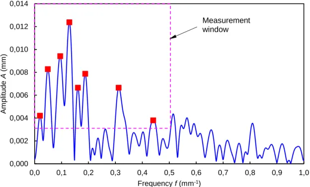
A total of 14 DFT spectra were analysed, 13 for the ply profiles (considering three double plies) and one for the plate profile. An example of the resulting DFT spectrum for the ply # 2 is shown in Figure 6.

Figure 6. DFT spectrum of the thickness profile of ply # 2 with selected frequency peaks (square markings). 0,000 0,002 0,004 0,006 0,008 0,010 0,012 0,014 0,0 0,1 0,2 0,3 0,4 0,5 0,6 0,7 0,8 0,9 1,0 A m pl itud e A (m m ) Frequency f (mm-1₎ Measurement window

The peaks of each spectrum are selected within a measurement window imposed by required finite element (FE) model mesh fineness which means it is impossible to model physics finer than the mesh itself. In this study, the measurement window is chosen to go from 0 to 0.50 mm-1 _{in frequency, and} from 0.0035 mm upwards in amplitude (cf. Figure 6). The analysis of the collected data was difficult due to the coupling of at least three variables, frequency, amplitude and phase shift, without mentioning that each profile spectrum contains a different number of peaks.

Therefore, to introduce the ply thickness variations into the FE model, a single set of N = 10 sine waves for all K plies (K = 16 for the present study) is created using an in-house pseudo-random generator of the zero-mean signal zk:

 

_





To have a precise control of the overall plate profile, the coupling of the ply thickness profiles is done by assigning a specific phase shift ϕn to each nth sine wave and each kth ply. As noted, the complete

dataset of the selected DFT peaks is divided into ten frequency bands of 0.05 mm-1 _{each from 0 to} 0.50 mm-1_{. A single frequency f}

n and amplitude An is obtained for each nth frequency band. After a

goodness-of-fit test for each nth _{band it was observed that the frequency values were better represented}

by a uniform distribution (with lower bound a and upper bound b limits) while the amplitude is better described by a normal distribution (with mean x̅ and standard deviation σ). It is noteworthy that not all

the frequency bands contain DFT peaks for all plies. For this reason, the parameter pn is drawn from a

binomial distribution with values being either 0 or 1. The probability to generate a value equal to 1 is the probability of appearance within the nth frequency band. The model parameters, which are obtained from the analysis of the different DFT spectra, are shown in Table 2.

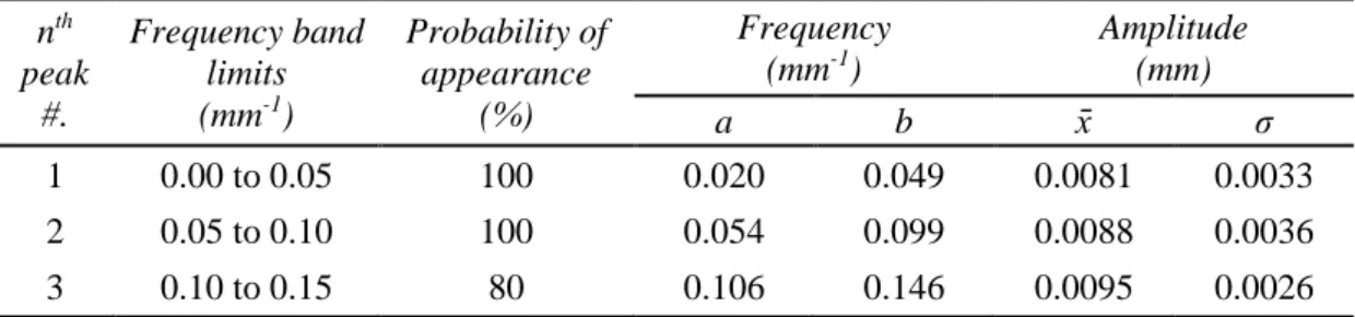
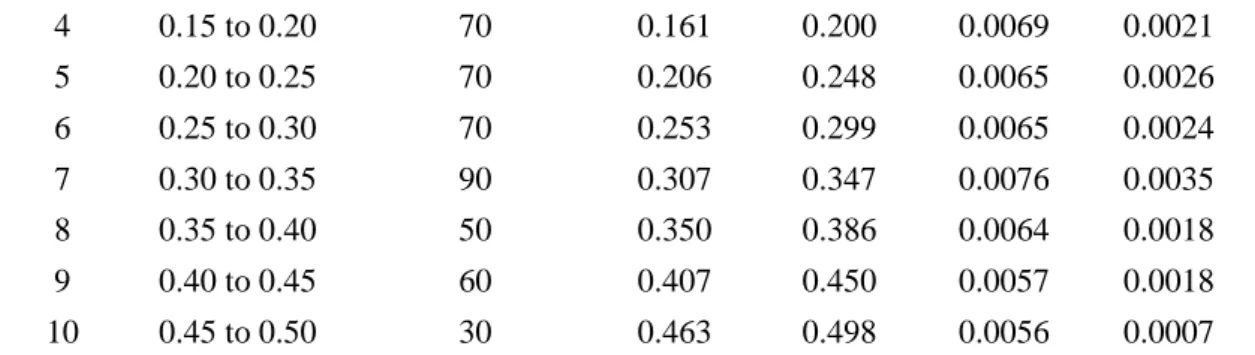
Table 2. Parameters of the distribution for the Frequency (uniform) and Amplitude (normal) associated with the probability of appearance of the nth _{peak within a frequency band.}

nth peak #. Frequency band limits (mm-1₎ Probability of appearance (%) Frequency (mm-1₎ Amplitude (mm) a b x̄ σ 1 0.00 to 0.05 100 0.020 0.049 0.0081 0.0033 2 0.05 to 0.10 100 0.054 0.099 0.0088 0.0036 3 0.10 to 0.15 80 0.106 0.146 0.0095 0.0026

4 0.15 to 0.20 70 0.161 0.200 0.0069 0.0021 5 0.20 to 0.25 70 0.206 0.248 0.0065 0.0026 6 0.25 to 0.30 70 0.253 0.299 0.0065 0.0024 7 0.30 to 0.35 90 0.307 0.347 0.0076 0.0035 8 0.35 to 0.40 50 0.350 0.386 0.0064 0.0018 9 0.40 to 0.45 60 0.407 0.450 0.0057 0.0018 10 0.45 to 0.50 30 0.463 0.498 0.0056 0.0007

4.2. Mathematical representation of ply thickness variations

The overall shape of the composite plate is controlled through the contribution of the thickness variation of the plate δt_pk. Nevertheless, the exact distribution of the thickness variations across the ply is difficult to know. However, the overall change of the composite plate δtp is known and it is evenly spread

over all the composite plies K, thus δt_pk can be estimated as:

K t tpk p



 

(3)

A 3D sine wave was chosen to be representative of the overall plate shape, δtp(x,y) is thus:

 









(4)

where Ap is the difference between the maximum and minimum thickness value, λ_px and λ_py are the plate

length and width respectively, and Xc and Yc are the desired coordinates of the maximum thickness zone.

Figure 7 shows the resulting thickness mapping on a 600 x 300 mm composite plate which is in good agreement, qualitatively and quantitatively, with the reality (cf. Figure 2).

Figure 7. Example of a numerical overall plate thickness generated using eq. 4.

The digital lay-up can be formed combining equations 1, 2 and 3 using the pseudo-random generator explained in section 4.1 and employing the parameters established in Table 2. The proposed model of each ply thickness adapted for a 3D representation is thus:

 

 

_

























f

x

f

y

A

p

K

y

x

t

t

y

x

t

sin

2

2

sin

4

,

,











where tk(x,y) is the generated thickness in both x and y-directions of the kth ply, t̄k is the mean thickness

of the kth _{ply, A}

n is the amplitude of the corresponding frequency fn for the nth peak, and np takes the value

1 or 0 depending on the probability of appearance of such nth _{peak. As previously explained, δt}

p(x,y) is

the desired plate profile divided by the number of plies, K.

To ensure a control on the coupling of the different ply thicknesses profiles, a pseudo random phase shift k,n is used for each kth ply and nth frequency peak. The overall plate profile (i.e. the sum of

the K ply profiles tk (x)) can maintained constant if the kth sum of the ply shifts must be equal for all nth

sinusoids (from 1 to N):















...





The phase shift ranges from -π to π for each nth _sinusoid: Length x (mm) W idt h y (m m ) 0 100 200 300 400 500 600 300 250 200 150 100 50 0 Plat e thic k nes s t p (m m ) 4.8 4.9 5.1 5.2 5.4 5.5

+

   kn  kn  K , , 2 (7)

where



4.3. Ply thickness generation discussion

The main goal of the digital thickness generator is not to reproduce the exact form of the composite ply spread over the plate, but to generate a geometry having the same characteristics, in terms of variability, as the actual ply thickness profiles. Even though the results associated with the proposed methodology (DFT spectra and range of values) are indeed dependent on the geometry, material and manufacturing conditions, the methodology itself does not depend on any of these conditions.

The variations found in the composite exhibit similar patterns but also exhibit differences compared with any point of the plates and with different plates manufactured with the same conditions. For this reason, the inclusion of random parameters into the mathematical representation allows the generation of new sets of virtual thicknesses that share the same characteristics in terms of variations than the studied plate.

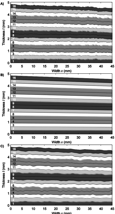
As observed in the cross-section of the composite material, the real stratification exhibits variations in the ply thickness (cf. Figure 8a). In the classic modelling of a composite stratification, the thickness of the different kth is considered as constant and it does not take in account the overall change in the stratification thickness (cf. Figure 8b).

Any effort made in order to completely model the behaviour of the thickness variation will take considerable computing and analytical resources since there are four highly interdependent variables that contribute to the thickness profile. The model must account for the number of the different frequencies and the spectral spacing between DFT peaks, the associated amplitude for each frequency and phase shifts. All these variables also depend on the ply position in the stratification. Different solutions to the problem, such as using the frequency values “as is” from one single ply, or randomly selecting the frequencies and their associated amplitudes from all the identified peaks were discarded, since the selected points come from a very specific zone in the plate that may or may not describe completely the

behaviour of the thickness variation along the full composite plate. Indeed, the data collection cannot be performed in all types of composite structures and for different composite plates due to its destructive nature, as well as the time and resources that this task demands. Therefore, simplifications must be made in order to obtain accurate data to be introduced into the model.

The variability of the ply thickness, as well as the coupling between the different plies to obtain a constant plate thickness, can be controlled by using pseudo-random algorithms to vary the parameters involved in the thickness profile generation (cf. Figure 8c).

Figure 8. Representation of the cross section of the 16 ply stratification (plies 4/5, 8/9 and 12/13 shown as independent plies) with, a) reconstruction from the actual ply thickness profiles (after filtering), b) constant

ply thickness accounting the contribution of the plate thickness variation in each ply and c) digital stratification generated by the proposed model.

5.

Determination of the material variations according with the geometrical

variations

Accounting for only thickness variations across the composite plate is not enough to determine their effect on local properties. The variation of volume fraction could be crucial since much of the thickness variation is due to differences in the amount of resin. This means that variations in properties could be less than the ones expected based on the thicknesses alone.

To introduce the local properties of the material linked to both ply thickness and the fibre volume fraction, the mass per unit area of the reinforcement ρ_Af is assumed constant over all the manufactured plates (i.e. for a given plate and from one plate to another). A micromechanical model of the fibre distribution along the ply could be implemented [14]. However, at the moment, it is difficult to determine with good precision this property due to the rearrangement of fibre bundles during the curing phase. Also the computation time would increase significantly. Assuming that the quantity of fibres cannot drastically vary along the reinforcement direction (in a continuous fibrous reinforcement), a rough and quick estimation of the fibre volume fraction V_fk(x,y) at any point in the stratification can be thus made without

the need of a micromechanical model of the fibre distribution inside the ply:

 

_{ }

y

x

t

t

y

x

V

,

,



(8)

where tk(x,y) is the local thickness in the xy-coordinates and in the kth ply, and an tf is the equivalent

thickness of the reinforcement defined by:

f A f f t   

(9)

where ρ_Af is the mass per unit area of the reinforcement and ρf the density of the reinforcement. Since both

parameters are considered constant, the equivalent thickness of the reinforcement tf is constant. The ρ_Af

value is calibrated to 305 g∙m-2 _{from observations of the M10.1/CHS manufactured plates.}

Finally, the volume fraction of the matrix V_mk(x,y) is given as follows:

 

x

y

V

 

x

y

V

 

x

y

V

k

where Vp(x,y) is the local volume fraction of porosity.

Subsequently, using the computed volume fractions and the constituent materials properties expressed in Table 3, the elastic properties are calculated by means of the classic law of mixtures.

Table 3. Mechanical properties of the CHS reinforcement and M10.1 resin.

Property Manufacturer values

Young’s modulus of the carbon fibre in the longitudinal

direction E_1f (GPa) 230

Young’s modulus of the carbon fibre in the transverse

direction E_2f (GPa) 15

Shear modulus of the carbon fibre G_{12f (GPa)} 50

Poisson’s ratio of the carbon fibre ν_{12f 0.28}

Density of the carbon fibre ρf (kg∙m-3) 1800

Mass per unit area of the carbon fibre ρ_Af (kg∙m-2₎

0.305 Coefficient of linear thermal expansion of the carbon

fibre α_{1f (°C}-1₎ - 1∙10-6

Young’s modulus of the epoxy resin Em (GPa) 3.6

Poisson’s ratio of the epoxy resin νm 0.3

Density of the epoxy resin ρm (kg∙m-3) 1200

Coefficient of linear thermal expansion of the epoxy

resin αm (°C-1) 25∙10

-6

The proposed modelling is only intended for obtaining a quick estimation of the material properties linked to the variation of the ply thickness. For this reason, it does not intend to model the lamina morphology (i.e. fibre bundles distribution, out-of-plane misalignments, porosity distribution, etc.). Nevertheless, the overall method does not exclude a more complete modelling of the lamina micromechanics depending on the available computational resources.

6.

Finite element modelling of the residual strains of a composite plate with

variable thicknesses.

The finite element (FE) model is required to be robust and light-weight. It uses a shell element type in the LMS Samcef® _{(Siemens, formerly Samtech, Belgium) code. The shell composite element} allows local control of the ply thickness for each element and each ply.

To illustrate of the capability to introduce local thickness variations into a FE model, a composite plate subjected to a temperature change of ΔT = -100 °C is presented as an example. This temperature

change is applied to calculate the residual strains at the end of the cooling phase during manufacturing. The analysis is typically based on the assumption that the composite is stress free at the curing temperature. Due to the mismatch of the thermal properties of the constituent materials, a temperature variation induces residual strains and stresses [15]. The complete 600 x 300 mm composite plate is analysed using a 2D Mindlin composite shell (element type T028/T029). The element size is set to be 1 mm per side in order to model a ply thickness undulation corresponding to a minimum wavelength of 2 mm (cf. Figure 6).

Three cases are analysed, the first one considers a constant plate and ply thicknesses. The second case uses variable laminate profiles generated by the algorithm explained in section 4.2 with constant material properties. For the third case, the ply and plate geometry is the same as case 2 but the material properties are calculated for each element and each ply as per section 5. The mean ply thickness for each plate is 0.30 mm, thus the plate thickness is 4.84 mm (cf. Figure 1). For all 3 cases, no porosity is assumed

Vp(x,y) = 0.

The deterministic solution without taking account of the thickness variations (case 1) shows as expected a uniform strain field εxx having a value of -83∙10-6 mm/mm marked as a reference value in

Figure 9. Figure 9 shows the strain field εxx of the upper skin for case 2 (Figure 9 top) and case 3

(Figure 9 bottom). The model without accounting for the material variations (cf. Figure 9 top) over estimates the compressive strains within a range of -80∙10-6 _{to -90∙10}-6 _{mm/mm. It is also evident that the} strain field forms uniform bands across the plate width. Conversely, the plates with variable thicknesses and variable materials (cf. Figure 9 bottom) exhibits a strain field with values ranging from -65∙10-6 _up to -85∙10-6 _mm/mm.

As shown, an attenuation of the residual strains is noticed, however the range of values Δεxx

passed from 10∙10-6 _{to 20∙10}-6 _{mm/mm, signifying an increase of an order of magnitude of the internal} variations. Also, the strain field distribution is completely different, with the most significant strains at the centre of the plate and a relaxation of such residual strains towards the corners of the plate.

Figure 9. Strain field εxx of the upper skin of a 16-ply 600 x 300 mm composite plate subject to a

ΔT = -100°C simulating the cooling process of a composite (top) no material variation assumed (bottom)

material vary according with thickness.

7.

Conclusions

The first input parameter towards the creation of a finite element model, affected by material variability, is the geometry variation of the ply thickness over the plate. Indeed, variations of this property impact the volume fractions of the constituent materials thus modifying the local material properties of the composite structure.

The thickness measurement of the composite plate studied reveals variations approximately Strain concentration

spots

Plate with thickness variations and constant material properties

Plate with thickness and material property variations

m m /m m m m /m m

2.5 times the thickness of a cured ply within the same composite plate. The observations made of the cross-section of the composite plate reveal continuous and periodic variations of the profiles and a non-linear coupling between the different ply thickness profiles and the resulting plate profile. This coupling is reflected by a low coefficient of variation (CV) of the plate thickness being less than ± 2 % of the mean plate thickness, while, the ply thicknesses exhibit a CV of 7 % of the mean ply thickness with maximal deviations up to ± 29 %.

A mathematical model of the ply variations is proposed to generate a digital laminate having similar dispersion on the ply thickness and having a strict control on the plate thickness shape. The frequency and amplitude values necessary to generate the digital ply are identified by the DFT analysis of the measured ply and plate thickness profiles. This modelling method produces ply thickness profiles having variations in accordance with the real ply and plate profiles.

The capabilities of the model are shown by computing the residual strains of the composite plate during the cooling phase of the autoclave processing. It is shown that accounting for geometrical and material variations generates a different strain field than for a classic composite plate without variations.

Acknowledgements

The authors would like to acknowledge CONACyT of Mexico for providing Yves Davila the financing for his PhD program. The authors would also give special thanks to Peter Davies for his invaluable comments and remarks.

References

1. Davila, Y.: Étude multi-échelle du couplage matériaux-procédés pour l’identification et la modélisation des variabilités au sein d’une structure composite. PhD Thesis. Université de Toulouse 3 Paul Sabatier (2015).

2. Barkanov, E., Gluhih, S., Ozolins, O., Eglitis, E., Almeida, F., Bowering, M.C., Watson, G.: Optimal weight design of laminated composite panels with different stiffeners under buckling loads. In: 27th International Congress of the Aeronautical Sciences. pp. 1–9 (2010).

3. Li, Y., Li, M., Gu, Y., Zhang, Z.: Numerical and Experimental Study on the Effect of Lay-Up Type and Structural Elements on Thickness Uniformity of L-Shaped Laminates. Appl. Compos. Mater. 16, 101–115 (2009).

4. Sun, J., Gu, Y., Li, Y., Li, M., Zhang, Z.: Role of Tool-Part Interaction in Consolidation of L-Shaped Laminates during Autoclave Process. Appl. Compos. Mater. 19, 583–597 (2011).

5. Lightfoot, J.S., Wisnom, M.R., Potter, K.: A new mechanism for the formation of ply wrinkles due to shear between plies. Compos. Part A Appl. Sci. Manuf. 49, 139–147 (2013).

6. Collombet, F., Mulle, M., Grunevald, Y.-H., Zitoune, R.: Contribution of Embedded Optical Fiber with Bragg Grating in Composite Structures for Tests-Simulations Dialogue. Mech. Adv. Mater. Struct. 13, 429–439 (2006).

7. Olivier, P., Cavarero, M.: Comparison between longitudinal tensile characteristics of thin and thick thermoset composite laminates: influence of curing conditions. Comput. Struct. 76, 125–137 (2000).

8. Li, Y., Li, M., Gu, Y., Zhang, Z.: Numerical and Experimental Study of the Bleeder Flow in Autoclave Process. Appl. Compos. Mater. 18, 327–336 (2010).

9. Hsiao, H.M., Daniel, I.M.: Effect of fiber waviness on stiffness and strength reduction of unidirectional composites under compressive loading. Compos. Sci. Technol. 56, 581–593 (1996). 10. Chun, H., Shin, J., Daniel, I.M.: Effects of material and geometric nonlinearities on the tensile and compressive behavior of composite materials with fiber waviness. Compos. Sci. Technol. 61, 125– 134 (2001).

11. Lee, M.C.W., Payne, R.M., Kelly, D.W., Thomson, R.S.: Determination of robustness for a stiffened composite structure using stochastic analysis. Compos. Struct. 86, 78–84 (2008). 12. Lee, M.C.W., Mikulik, Z., Kelly, D.W., Thomson, R.S., Degenhardt, R.: Robust design – A

concept for imperfection insensitive composite structures. Compos. Struct. 92, 1469–1477 (2010). 13. Olave, M., Vanaerschot, A., Lomov, S. V, Vandepitte, D.: Internal Geometry Variability of Two Woven Composites and Related Variability of the Stiffness. Polym. Compos. 1335–1350 (2012). 14. Yuanchen Huang, Kyo Kook Jin, Sung Kyu Ha: Effects of Fiber Arrangement on Mechanical

Behavior of Unidirectional Composites. J. Compos. Mater. 42, 1851–1871 (2008).

15. Mulle, M., Collombet, F., Olivier, P., Zitoune, R., Huchette, C., Laurin, F., Grunevald, Y.: Assessment of cure-residual strains through the thickness of carbon–epoxy laminates using FBGs Part II: Technological specimen. Compos. Part A Appl. Sci. Manuf. 40, 1534–1544 (2009).