Bearing capacity of foundations resting on a spatially random soil

HAL Id: hal-01007936

https://hal.archives-ouvertes.fr/hal-01007936

Submitted on 21 Oct 2018

HAL is a multi-disciplinary open access

archive for the deposit and dissemination of

sci-entific research documents, whether they are

pub-lished or not. The documents may come from

teaching and research institutions in France or

abroad, or from public or private research centers.

L’archive ouverte pluridisciplinaire HAL, est

destinée au dépôt et à la diffusion de documents

scientifiques de niveau recherche, publiés ou non,

émanant des établissements d’enseignement et de

recherche français ou étrangers, des laboratoires

publics ou privés.

Bearing capacity of foundations resting on a spatially

random soil

Abdul-Hamid Soubra, Dalia Youssef Abdel Massih, M. Kalfa

To cite this version:

Abdul-Hamid Soubra, Dalia Youssef Abdel Massih, M. Kalfa.

Bearing capacity of foundations

resting on a spatially random soil. Geocongress 2008, ASCE, 2008, New Orleans, United States.

�10.1061/40971(310)8�. �hal-01007936�

Bearing capacity of foundations resting on a spatially random soil

Abdul-Hamid Soubra1, Dalia S. Youssef Abdel Massih2and Mikaël Kalfa3

1

Professor, University of Nantes, GeM, UMR CNRS 6183, Bd. de l’université, BP 152, 44603 Saint-Nazaire cedex, France. E-mail: Abed.Soubra@univ-nantes.fr

2_{PhD Student, University of Nantes & Lebanese University, BP 11-5147, Beirut, Lebanon. E-mail:}

Dalia.Youssef@univ-nantes.fr

3_{Post Graduate Student, University of Nantes, GeM, UMR CNRS 6183, Bd. de l’université, BP 152,}

44603 Saint-Nazaire cedex, France

ABSTRACT: The paper presents the effect of the spatial variability of the soil properties on the ultimate bearing capacity of a vertically loaded shallow strip footing. The deterministic model used is based on numerical simulations using the Lagrangian explicit finite difference code FLAC3D. The cohesion and the angle of internal friction of the soil are modelled as non normal anisotropic random fields. The methodology used for the discretization of the random fields is based on the spectral representation method proposed by Yamazaki and Shinozuka (1988). The results have shown that the average bearing capacity of a spatially random soil is lower than the deterministic value obtained for a homogeneous soil. A critical case appears when the autocorrelation distances are equal to the footing breadth. The average value of the ultimate footing load is more sensitive to the horizontal autocorrelation distance than the vertical one. Finally, it has been shown that accounting for the spatial variability of the soil properties gives a higher reliability index of the foundation than the one obtained with the assumption of random variables.

INTRODUCTION

The spatial variability of the soil properties may largely affect the behaviour of geotechnical structures. This variability is widely dealt with as uncertainties in soil properties. Several authors have investigated the reliability-based analysis of foundations. Some authors have modelled the uncertainties of the different parameters as random variables (e.g. Low and Phoon 2002) without introducing the spatial variability of the soil parameters. Others (Cherubini 2000) have considered the effect of the soil spatial variability by using a simplified approach. Later on, several authors (Griffiths et al. 2002, Fenton and Griffiths 2003 and Popescu et al. 2005 among others) have modelled the uncertain soil parameters as random processes more rigorously. They have examined the effect of the spatial variability of these parameters on the ultimate bearing capacity using finite elements models combined with Monte Carlo simulations. However, most of these studies (except Fenton and Griffiths 2003) consider only a single random process in their analysis.

In this paper, the effect of the soil spatial variability on the reliability analysis and design of a vertically loaded strip foundation is presented. The punching mode of the

ultimate limit state is analyzed. Only the cohesion and the angle of internal friction of the soil are modelled as non normal anisotropic random fields. The cohesion is considered to be Log-normally distributed while the angle of internal friction follows a Beta distribution. Several realisations of the random fields are performed using Monte Carlo simulations. The methodology used for the discretization of the non-gaussian random fields is based on the spectral representation method proposed by Yamazaki and Shinozuka (1988). This method is fast, easy to apply and allows one to take into account the soil anisotropy regarding the autocorrelation distances.

After a brief description of the methodology used in this paper, the deterministic model is first described and then, the stochastic numerical results are presented and discussed.

METHODOLOGY

Generation of non-Gaussian random fields

The approach described by Popescu et al. (1998) based on the spectral representation method was used to generate sample functions of a 2D non-Gaussian stochastic vector field according to a prescribed spectral density function and a prescribed (non-Gaussian) probability distribution function. It should be mentioned

that the spectral density functionS

( )

( )

of the random process by the following relation:

( )

( )

First a Gaussian vector field is generated according to the target spectral density function using the Fast Fourier Transformation (FFT) algorithm. Next, this Gaussian vector field is transformed into the desired non-Gaussian field using a memory less non-linear transformation coupled with an iterative process. For the description of the theoretical bases of the spectral representation method, one can refer to Shinozuka and Deodatis (1991) and Popescu et al. (1998).

Monte Carlo simulations

For each set of assumed statistical parameters of the soil properties random fields, several realizations of the random field are generated in Matlab 7.0 by the spectral representation method using Monte Carlo simulations. The bearing capacity and the slope of the foundation corresponding to each realisation are calculated based on

numerical simulations using the Lagrangian explicit finite difference code FLAC3D.

The data transfer from the stochastic mesh used to generate the random fields to the

finite difference mesh of FLAC3Dis performed using the mid point method. The

unbiased mean and standard deviation of the footing load are obtained using the following equations: 1 1 sim u n P u i sim P n µ = = (2)

(

)

where nsimis the number of the sample size of the random field realizations.

An exchange of data between FLAC3D and Matlab 7.0 in both directions was

necessary to enable an automatic resolution of the Monte Carlo simulations for the generation of the soil properties random fields and the calculation of the geotechnical

system responses (i.e. ultimate footing load, footing displacement, footing slope). The

link between FLAC3D and Matlab 7.0 was performed using text files and FISH

commands. FISH is an internal programming option of FLAC3Dwhich enables the

user to add his own subroutines. DETERMINISTIC MODEL

The deterministic model used for the calculation of the ultimate footing load, the vertical footing displacement and the footing slope is based on numerical simulations

using FLAC3D. A soil domain of width 15B and depth 2.5B is considered (Figure 5).

The bottom and right vertical boundaries are far enough from the footing and they do not disturb the soil mass in motion (i.e. velocity field) for all the soil configurations studied in this paper. A non uniform optimized mesh composed of 1620 zones is used (Figure 5). Since this is a 2D case, all displacements in the Y direction (see Figure 5) are fixed. For the displacement boundary conditions, the bottom boundary was assumed to be fixed and the vertical boundaries were constrained in motion in the horizontal direction. A conventional elastic-perfectly plastic model based on the Mohr-Coulomb failure criterion is used to represent the soil. A strip footing of width equal to 2m and depth 0.5m is simulated by a weightless elastic material. It is divided horizontally into eight zones. The footing elastic properties used are the Young’s

modulus E=25 GPa and the Poisson’s ratio =0.4. Compared to the soil elastic

properties (E=240MPa, =0.2), these values are well in excess of those of the soil and ensure a rigid behavior of the footing. The footing is connected to the soil via interface elements that follow Coulomb law. The interface is assumed to have a friction angle equal to the soil angle of internal friction, dilation equal to that of the soil and cohesion equal to the soil cohesion in order to simulate a perfectly rough soil-footing interface. Normal stiffness Kn=109Pa/m and shear stiffness Ks=109Pa/m are

assigned to this interface. These parameters do not have a major influence on the failure load.

For the computation of the bearing capacity of a rigid rough strip footing subjected

to a central vertical load using FLAC3D, the following method is adopted: an optimal

controlled downward vertical velocity of 5.10-6 m/timestep (i.e. displacement per

timestep) is applied to the bottom central node of the footing in order to allow the rotation of the footing due to the soil spatial variability (i.e. soil variability). Damping of the system is introduced by running several cycles until a steady state of plastic flow is developed in the soil underneath the footing. At each cycle, the vertical footing load is obtained by using a FISH function that calculates the integral of the normal stress components for all elements in contact with the footing. The value of the vertical footing load at the plastic steady state is the ultimate footing load. NUMERICAL RESULTS

The numerical results presented in this paper consider the case of a shallow strip foundation with breadth B=2 m subjected to a central vertical load. The soil has a unit

weight of 18 kN/m3. The cohesion and the angle of internal friction are modeled as

two independent random fields. The illustrative values used for the statistical

moments of c and are as follows: µc=20kPa,

o 30 = µ , COVc =20%, % 10 =

COV . The dilation angle was taken equal to 2 3. For the probability

distributions of the random fields, c follows a log-normal distribution while is

An anisotropic autocorrelation function is used in this paper for both the cohesion and the angle of internal friction. It is given by an exponential first order function as follows (e.g. Vanmarcke, 1983):

(

)

where Dh and Dv are the autocorrelation distances in the horizontal and vertical

directions respectively and, x and y are the lag distances in the horizontal and

vertical directions respectively.

Convergence of the Monte Carlo simulations

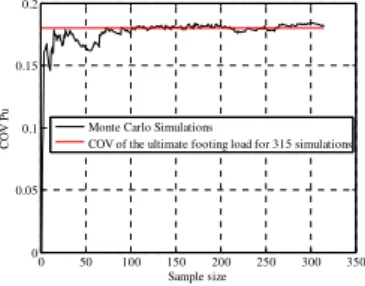
Figures (1) and (2) show the effect of the sample size on the predicted mean µ_Pu

and coefficient of variationCOVPu of the ultimate footing load. The case considered in

these figures corresponds to an isotropic autocorrelation function with x = y =2 m.

It can be seen that the predicted mean and coefficient of variation remain practically constant for sample size larger than 100. Consequently, only 100 realizations of the soil properties random fields are used in all subsequent calculations. For this number,

estimated mean bearing capacities will have a standard error (± one standard

deviation) equal to the sample standard deviation times 1 nsim =0.1, or 10% of the

sample standard deviation. Similarly, the estimated variance will have a standard error equal to the sample variance times

(

)

variance. This means that estimated quantities will generally be within about 14% of the true quantities.

0 50 100 150 200 250 300 350 2.05 2.1 2.15 2.2 2.25 2.3 2.35 2.4 2.45x 10 6 Sample size µPu(N /m )

Monte Carlo simulations

Mean of the ultimate footing load for 315 simulations

0 50 100 150 200 250 300 350 0 0.05 0.1 0.15 0.2 Sample size C O V P u

Monte Carlo Simulations

COV of the ultimate footing load for 315 simulations

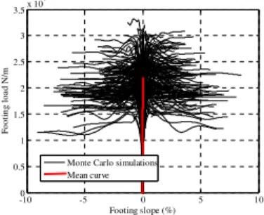
Figure (3) and (4) present respectively the displacement curves and the load-slope curves of the footing obtained for all the soil realizations of the Monte Carlo simulations. These figures also present the mean curves of all simulations. It can be noticed that the mean value of the footing slope is very close to zero. However, the footing slope corresponding to each realization is different from zero. Figure (5) shows the deformed mesh obtained for a random soil realization. This figure shows that the inherent spatial variability of the soil shear strength parameters can modify drastically the basic form of the failure mechanism. Differential settlements appear in

FIG. 1: Mean of the ultimate footing load versus the sample size

FIG. 2: Standard deviation of the ultimate footing load versus the sample size

the spatially varying soil leading to the rotation of the footing. This is impossible in a deterministic homogeneous soil analysis of a symmetrical problem.

0 0.01 0.02 0.03 0.04 0.05 0.06 0.07 0.08 0.09 0 0.5 1 1.5 2 2.5 3 3.5x 10 6 F o o ti n g L o a d (N /m ) Footing Displacement (m) Monte Carlo Simulations Mean curve -100 -5 0 5 10 0.5 1 1.5 2 2.5 3 3.5x 10 6 Footing slope (%) F o o ti n g lo a d N /m

Monte Carlo simulations Mean curve

FIG. 5: Deformed Mesh corresponding to a realization of the random soil Predicted mean and standard deviation of the ultimate footing load

Figures (6) and (7) show respectively, in a dimensionless form, the variation of the predicted mean and standard deviation of the ultimate footing load with the

autocorrelation distance for an isotropic random soil (i.e. x = y) and for different

values of the coefficient of variation of the random fields.

29 29.5 30 30.5 31 31.5 32 32.5 33 33.5 0.1 1 10 100 1000 /B µ P u / B 2

Deterministic ultimate footing load COVc=20%; COV =10% COVc=40%; COV =10% COVc=20%; COV =15% 0 2 4 6 8 10 12 14 16 0.1 1 10 100 1000 /B P u/ B 2 COVc=20%; COV =10% COVc=40%; COV =10% COVc=20%; COV =15%

One can notice that the average bearing capacity of a spatially random soil is lower than the deterministic value obtained for a homogeneous soil for which the soil properties are set equal to their mean values. A critical case appears in figure (6) when the autocorrelation distances are close to the footing breadth. For this case, the curve of the mean value of the footing load reaches a minimum. This case was also obtained in Fenton and Griffiths (2003). Concerning the standard deviation of the ultimate

FIG. 7: Standard deviation of Pu

versus the autocorrelation distance (isotropic random soil)

FIG. 6: Mean value of Puversus

the autocorrelation distance (isotropic random soil)

FIG. 3: Load-displacement curves from Monte Carlo simulations

FIG. 4: Load-slope curves from Monte Carlo simulations

footing load, it always increases with the increase of the autocorrelation distances. From the two figures, one can conclude that the statistical parameters of the bearing capacity are more sensitive to the variation of the angle of internal friction than the cohesion.

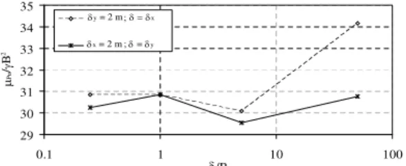
Effect of the vertical and horizontal autocorrelation distances on the mean value of the ultimate footing load

Figure (8) presents the variation of the mean ultimate footing load with the vertical and horizontal autocorrelation distances. For each curve in figure (8), one autocorrelation distance is set equal to 2 m and the second one varies from

0.5 m

B= to B=50 m. It can be noticed that the mean ultimate footing load is

more sensitive to the variation of the horizontal autocorrelation distance than the vertical one. 29 30 31 32 33 34 35 0.1 1 10 100 /B µ P u / B 2 y= 2 m; = x x= 2 m ; = y

FIG. 8: Mean value of the ultimate footing load versus the autocorrelation distances for an anisotropic random soil

0.5 1 1.5 2 2.5 3 3.5 4 x 106 0 0.2 0.4 0.6 0.8 1 1.2 1.4x 10 -6 Pu (N/m) P D F Monte Carlo Normal distribution Gamma distribution Lognormal distribution

FIG. 9: Histogram and fitted probability density distributions of the ultimate footing load

Reliability index

By fitting the histogram of the ultimate footing load obtained from the Monte Carlo simulations to an empirical probability density function [Normal (N), Lognormal (LN), Gamma (G)] (cf. Figure 9), one can approximate the reliability of the footing, subjected to a prescribed service applied load Ps, against punching failure

by calculating the Hasofer-Lind reliability index as follows:

2143.5 kPa Pu

µ =

401.29 kPa

1 min u u u u u u s N N P P S P HL P N N P P P x µ P µ = = (6) where et u u N N P P

µ are respectively the equivalent normal mean and standard deviation

of the ultimate footing load.

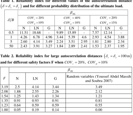
Table 1 shows that the reliability index decreases with the increase of the autocorrelation distances. Consequently, accounting for the spatial variability of the soil properties gives a higher reliability index than the one obtained with the assumption of random variables. Table 2 presents a comparison between the

reliability index values obtained for large autocorrelation distances

(

)

(2007). In the later reference, the soil shear strength properties were modeled by random variables and the response surface methodology was used to calculate the

reliability index based on FLAC3D_{simulations. A good agreement between the two}

results was noticed when assuming a Gamma distribution for the ultimate footing. Table 1. Reliability index for different values of the autocorrelation distance

(

)

HL 20% 10% c COV COV = = 40% 10% c COV COV = = 20% 15% c COV COV = = B N LN G N LN G N LN G 0.5 11.51 18.68 - 9.89 15.89 - 7.57 12.14 -1 4.26 6.78 4.96 3.44 5.39 4.6 2.93 4.54 3.88 5 2.60 4.14 3.49 2.24 3.51 2.95 1.81 2.80 2.34 50 2.43 3.91 3.27 1.84 2.89 2.41 1.53 2.37 1.95

Table 2. Reliability index for large autocorrelation distances

(

)

CONCLUSIONS

The paper presents the effect of the spatial variability of the soil shear strength parameters on the ultimate bearing capacity of a vertically loaded shallow strip footing. The deterministic model used is based on numerical simulations using the

Lagrangian explicit finite difference code FLAC3D. The cohesion and the angle of

internal friction of the soil are modelled as non normal anisotropic random fields. The HL

F N LN G Random variables (Youssef Abdel Massih

and Soubra 2007) 3.19 2.5 4.14 3.44 3.49 2.08 1.88 2.55 2.26 2.12 1.54 1.25 1.43 1.34 1.21 1.35 0.91 0.93 0.91 0.81 1.23 0.64 0.59 0.59 0.55 1.00 0.05 0.19 0.14 0.00

cohesion is considered to be Log-normally distributed while the angle of internal friction follows a Beta distribution. An anisotropic exponential first order autocorrelation function is used in this paper for the two random processes. Several realisations of the random field are generated by the spectral representation method using Monte Carlo simulations. The ultimate footing load was calculated for all the realisations. The results have shown that the inherent spatial variability of the soil shear strength parameters can modify drastically the basic form of the failure mechanism. Differential settlements appear in the spatially random soil leading to the rotation of the footing. This is impossible in a deterministic homogeneous soil analysis of a symmetrical problem. The average bearing capacity of a spatially varying soil was found lower than the deterministic value obtained for a homogeneous soil. A critical case appears when the autocorrelation distances are equal to the footing breadth. It was found that the statistical parameters of the bearing capacity are more sensitive to the variation of the angle of internal friction than the cohesion. Also, the average value of the ultimate footing load was found more sensitive to the variation of the horizontal autocorrelation distance than the vertical one. The probability distribution of the bearing capacity was analysed. Several types of the probability distribution function were fitted to the histogram of the obtained bearing capacities. After assuming a probability distribution for the ultimate foundation load, a reliability analysis was performed. The Hasofer-Lind reliability index was calculated for the assessment of the footing reliability. It was found that accounting for the spatial variability of the soil properties gives a higher reliability index than the one obtained based on the assumption of random variables.

REFERENCES

Cherubini, C. (2000). "Reliability evaluation of shallow foundation bearing capacity on_{c ,}' ' _{soils." Can. Geotech. J., 37, 264-269.}

Fenton, G. A., and Griffiths D. V. (2003). "Bearing capacity prediction of spatially random c- soils." Can. Geotech. J., 40, 54-65.

Griffiths, D. V., Fenton, G. A., and Manoharan, N. (2002). "Bearing capacity of rough rigid strip footing on cohesive soil: Probabilistic study." J. of Geotech. & Geoenv.

Engrg., ASCE, 128(9), 743-755.

Low, B. K., and Phoon, K. K. (2002). "Practical first-order reliability computations using spreadsheet." Probabilistics in Geotechnics: Technical and Economic Risk

Estimation, Austria, 39-46.

Popescu, R., Deodatis, G., and Prevost, J.H. (1998). "Simulation of homogeneous non-Gaussian stochastic vector fields" Prob. Engrg. Mech., 13(1), 1-13.

Popescu, R., Deodatis, G., and Nobahar, A. (2005). "Effect of random heterogeneity of soil properties on bearing capacity." Prob. Engrg. Mech., 20, 324-341. Shinozuka, M., and Deodatis, G. (1988). "Response variability of stochastic finite

element systems." Journal of Engineering Mechanics, 114(3), 499-519.

Shinozuka, M., and Deodatis, G. (1991). "Simulation of stochastic processes by spectral representation." Applied Mechanics Reviews, ASME, 44(4), 191-204. Vanmarcke, E. (1983). "Random Fields: Analysis and Synthesis." Published by MIT

Press, Cambridge MA, 382p.

Yamazaki, F., and Shinozuka, m. (1988). "Digital generation of non-Gaussian stochastic fields." J. of Engrg. Mech., 114(7), 1183-1197.

Youssef Abdel Massih, D.S., and Soubra, A.-H. (2007). "Reliability-based analysis of strip footings using response surface methodology." Int. J. of Geomech., ASCE, accepted, in press.