On the (Mis)Specification of Seasonality and Its Consequences: an Empirical Investigation with U.S. Data

(1)

ON THE (MIS)SPECIFICATION OF

SEASON!Y,ITY AND

rrs

CONSEQUENCES :

AN EMPIRICAL INVESTIGATION WITH U.S. DATA

Eric Ghysels1, Hahn

S.

Lee2 _and_{Pierre L Siklos}3

1 _{Departement de sciences economiques and Centre}

_de

_{recherche et} developpement

en

economique (C.RD.E.), Uoiversit.e de

Montreal ..

2

_Department

_of

_Economics,

_{Tulane University.}

3

_Depar1ment

_of

_{Economics, Wilfrid}

_{Laurier University.}

December 1992

The first author would like to acknowledge the financial support of the SSHRC and

NSERC

of Canada. as well

as

the Fonds FCAR

of ~bee.

Part

of this paper was done while the first author

was

on sabbatical leave at

the

Cowles Foundation, Yale University.

Its

financial support and hospitality

are

also gratefully acknowledged. The third author is grateful for the hospitality of

the

University of California, San Diego where he was a visiting scholar during the

spring

of

1991, to Wilfrid

Laurier University for financial support through a short-term research grant. a Course

Remission

Grant and

the

Academic

Development Fund. Comments

by

an anonymous referee on an earlier draft helped improve the

paper.

A companion C.R.D.E. (Universite de Montreal) wolking paper

with

a more detailed account of the empirical results is available upon request.

C.P. 6128. sucanaleA Monlrul(au.bec) H3C3J7.

T6le<:opiour (FAX): (51•) 3"3-5831

(2)

Ce

cahier a egalement e~ publi6

par

le

Centre

de recherche

et

~v~Jo

6:onomique de l'Universi~ de Montreal (publication no 4692). :

Depot legal -

quattreme trimestre

1992

Biblioth~ue nationale du

Canada

8'ries

ou

ron a enlew la tendance (e.g., Nelson et Kang (1981)). Les procedures d'ajustemert : saisonnier sont baSNS sur des hypotheses implicites ou explicites sur les racines au

cercle-unite, aux fr~uences saisonnieres et A la fr~uence zero. En consequence, les procedures d'ajustement saisonnler peuvent produire un faux "detrending' et d'autres effets statistiquement lndesirables.

Dans ce papier, on examine, pour une large classe de series trimestrielles de donnees macroeconcmiques am6ricaines. les effets de differentes procedures d'ajustement salsonnier sur les proprietes de series univariees ajustees. Nous considerons egalement quelles -proc4dures sont appropriees, etant donne les proprietes des

donnees.

Dans rensemble, nous detectons des differences tres slgnificatives alnsl que rlWidence de faux cycles dans les series filtrees par differentes procedures. Nous presentons dgalement une extension des procedures de selections de modeles dans les tests du type ADF, propose par Hall (1990),

a

des tests du

~ type HEGY •

. · Mots cles : desaisonnalisation

et

faits stylises, procedures de test ,HEGY, selection de modele

basee

sur l'echantillon, tests de racine unitaire.

ABSTRACT

It

is well known that misspecification of a trend leads to spurious cycles in detrended data '.:(see, e.g., Nelson and Kang (1981)). SeasonaJadjustmentproceduresmakeassumptions, either

• 'Implicitly or explicitly, about roots on the unit circle both at the zero and seasonal frequencies. Consequently, seasonal adjustment procedures may produce spurious detrending and other : statistically undesirable effects.

In this paper,

we

document, for a large class of widely used U.S. quarterly macroeconomic , series, the effects of competing seasonal adjustment procedures on the univariate time series 'properties of adjusted series. We also investigate which procedures

are

most appropriate, given

the

properties of the data. Overaff,

we

find very significant cflfferences and evidence of spurious , cycles among series filtered via different adjustment procedures. A byproduct of our paper is

.. an

extension of data-dependent model selection rules in ADF tests, proposed

and

analyzed by

Hall (1990), to HEGY-type procedures.

: Key words : seasonal adjustments and stylized facts, HEGY test procedures, data-based model selection, unit root tests.

(3)

1. lntroducUon

Misspecification of a trend leads to spurious cycles in detrended data, as for instance Nelson and Kang (1981) emphasized. What is perhaps less obvious is the fact that seasonal adjustment procedures may produce similar effects. This paper takes up the question whether spuriousness is a problem when seasonals are removed via an adjustment procedure based on a misspecified model ol seasonality.

There exists, of course. a vast literature about the ideal properties seasonal adjustment procedures should have, ilcluding the fact that they should leave the time series properties of the series unaffected except al the seasonal frequencies (see e.g. Nerlove

et

al. (1979), Bell and Hillmer (1984) and Hylleberg (1986) for surveys and detailed discussion). As is now well known, many time series are ncinstationary and they are widely believed to contain a unit root at the zero frequency (see CampbeU and Perron 1991 for a recent survey). Similarly, usual seasonal adjustment procedures make either implicitly or explicitly assumptions about roots on the unit circle both at the zero as

wen

as at the seasonal frequency and its harmonics. TypicaUy. in applied research, adjustment for seasonality assumes that seasonality is deterministic and can be removed via

seasonal dummies thus ignoring the possibility ol the stochastic and nonstationary nature of seasonality. On the other hand, the commonly applied monthly Census X· 11 program, for instance, implies dala transformations which include the (1

+ L

+

L2

_{+ .... +}

_L11, where L1, is the lag operator for I periods) filter, resulting in a •removar of unit roots at the monthly seasonal frequency and its harmonics.1

Data transformations thal go along with the removal of seasonals may or may not be approprlale, just like trend removal can be inadequately done. In this paper we document for a large class of quarterly U.S. Post World War II time series how several of the data transformations typically associated with seasonal adjustment affect the univariate time series properties of interest

to

economists. such as the autocorrelation and

partial autocorrelation functions of the transformed data. In addition, we use tests proposed by Hylleberg, Engle, Granger and Yoo (1990; henceforth HEGY) to determine which dala transformation appears

to

be most appropriate.

(4)

With

one

exception. aD the data transformations we consider Imply the

same

treatment

with regard to

zero

fraquency detrending. Namely, all transformations

assume

the data have a unit

root

at the zero frequency except for the case where

a

first

difference is combined with a seasonal difference. In the latter case we obtain two unit roots at the zero frequency. All seasonal adjustment data transformations differ,

however.

with regard to the treatrwlt of

deterministic

and stochastic seasonality and the

presence

of unit

root

at seasonal frequencies In the stochastic case. In general, It Is found

that

summary statistics of the data 818 quite sensitive to the way seasonal adjustment Is applied. Very dfferanl conclusions can be found for the univariate characterization of the data depending on the way seasonals are elinmated even with the detrending being kept

constant across different adjustment procedures.

A by-product of our paper is a theoretical extension of the HEGY procedure.

As_

they

involve· an AR polynomial expansion. similar to Dlckey-Funer tests for unit roots at tha

zero

frequency,

one

has to select a lag length to calculate the tests. Recently, HaN

(1990) derived tha limiting

distribution

of tha augmented Dickey-Fuller test when the AR polynomial expansion is chosen usi,g data-based methods, as is most often donein practice. We extend Hairs zero fraquency results to HEGY tests for unit roots at tha

zero

and seasonal frequencies. . ' ·'

It may be worth emphasizing

a

few limitations of our paper. We wiU only disc~

'ti.a

effect of filtering on the univariate characterization of data and not the consequen&,~1of d,_:,;'4

filtering on estimation and testing. Hence, we wiU not elaborate on the

Issue of filtering

and estination and 1estSlg, In part because this subject Is documented In detail In for

t:<:'"i i'.

instance Sins (1974), Wallis (1974). Sins (1985), Ghysels and Perron (1992), Hansen.•

. --~·¢··'

and Sargent (1992), Sins (1992), among others. · ·-". ·

' - .,-·.·-~.,,_ ~

The paper is

organized

as

follows.

In Section 2 we criscuss the autocorrelation and ..

. ~ - ·:-,, --;:'/{fti.! ./.

partial autocorrelation functions of a representative set of U.S. quarterly time series after ..

. . "·. ,;:;,;,,tl/t , .

being adjusted . with a set of five commonly used filters for removal of

'seasons' .

. ,~ . :~ .. "')ff~{,"-:.

fluctuations.

Next. we

present a summary of the HEGY procedure and extend it to

aUo

· • .;;,.t.cif

for data based augmentation lag selection. Empirical results of the HEGY procedure are

reported in Section 3. Conclusions appear in Section 4.

2. Univariate Time Serles Properties of U.S. Quarterly Data

Quarterly data on a variety of U.S. macroeconomic series were considered similar to Barsky and Miron (1989; hereafter BM) whose sample usuaUy begins in 1946 and ends in 1985 (see their Table 1). Not all of the series used by BM were considered in this

paper. We omitted the components of flXed Investment expenditures, the money multiplier, state and local government spending. and final sales. However, we added per

capita versions of GNP and consumption expenditures and its components as well as a measure of real balances.2 _{We did,}

_however,

_also_{update the data}_used_{by BM up to}

tha fourth quarter of 1989. In the results reported below,

we

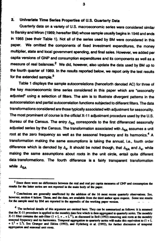
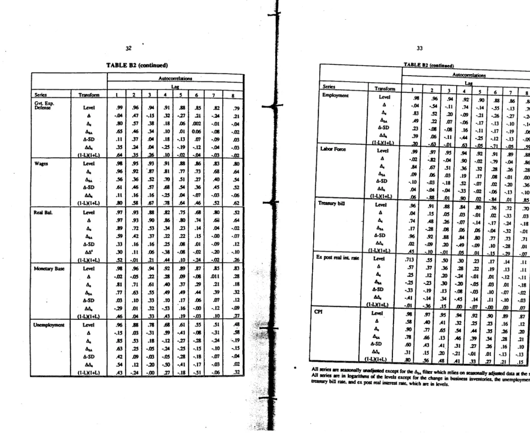
report only the test resuNs for the extended sample.3

Table 1 displays the sample autocorrelations (henceforth denoted AC) for three of

tha key macroeconomic time series considered in this paper which are •seasonally adjusted" using a selection of filters. The aim Is to tnustrate divergent patterns in tha

autocorrelation and partial autocorrelation functions subjected to <frfferent filters. The data transformations considered are those typically associated with adjustment for seasonality. The most prominent of course Is the official X-11 adjustment procedure used by the U.S. Bureau of the Census. The entry AsA corresl)Oflds to the fll'SI <frfferenced seasonally adjusted series by the Census. The transformation associated with ~ assumes a unit root at the zero frequency as wen as the seasonal

frequency

and its harmonics.4 _A

transformation making the same assumptions is taking the annual, I.e., fourth order difference which is denoted by A4. It should be noted lh<>ugl, that AsA and A4, while

making tha same assumptions about roots in the unit circle, entail quite <frfferent data transformations. The fourth difference is a fairly transparent transformation while~

2 _Since_{dlcre -} _{no diffcrmces}_betMm_Ille_ia1_and_ial_per_{c:apila -} _of_{GNP and}_{CXlllSlllllplio Ille} n:suhs for the laaa series me not RP)l1Cd ia die maia body of die JIIIICS'.

3 Coac1usicas me gcaera11y -'Teaed by die addi1ion of die 16 - n:aat quanerfy obsenalions. See.

boweYer. lCCtion 4 llelow. These, and die - - - available from die lllird aadlor 11p011 request. Some lest iesults

for.die ample med by BM me ieponed in Ille ll'l)elldh of die worting JIIIICS' 'ICISion. . - ,. 4 _{The l«hnical}_details_{of Ibis}_{argument me}_ooiilted_llae._Tbey_can_be_{srmmariud as}_{follows: it}_{is assumed} lllat die X-11 procedure is applied 1o the moadlly data rnt which is d i m ~ to qua,taty series. 1bc mmllly X-11 filterconlains die sub-filter(!+ L + _ + L11). as discussed ia BcD (1992) ranoring unit roocs • die ~ l y seasonal ~ and ilS harmonies. Temporal aggqalioa te quanaty eries will-mate this ai,ii'V81ent lo (I + L

+ L2 + L 3). Sec Granger and Sitlos (1992), ac1 Hylleberg et al (1992), for fwtber discussion of lelllpOnl au,eption and - i unit ronlS.

(5)

Series GNP

Cons.

M1

TABLE 1

Autocorrelatlons of Soma Key Macroeconomic Variables

with Different Seasonal AdjUS1ment FIiters

Autocorrelations Lag Transfonn 1 2 3 4 5 6 7 Level .98 .96 .94 .92 .90 .89 .87 A -.60 .34 -.61 .90 -.63 .32 -.60 A4 .83 .54 .22 -.06 -.18 -.16 -.07 ~ .37 .25 .00 -.10 -.12 -.06 -.02 A-SD -.02 -.003 -.15 .38 •.28 -.13 •.15

Mc

.32 .12 -.12 -.46 -.36 -.21 -.07

level

~98 .97 .95 .93 .92 .90 .88 A -.68 .41 -.67 .94 -.65 .39 -.65 A4 .78 .65 .50 .32 .33 .30 .35 ~ .05 .22 .04 -.03 -.06 -.12 .05 A-SD -.41 .30 -.38 .61 -.30 .19 -.32 M4 -.22 .13 .03 -.43 .11 •.21 .08 M4 -.20 .14 .08 -.37 .14 -.21 .10 Level .98 .96 .94 .91 .89 .87 .84 A .10 -.15 .01 .72 .02 -.16 -.05

A.c

.92 .80 .67 .56 .50 .46 .41 ~ .57 .40 .30 .17 .29 .26 .09 A-SD .36 .16 .21 .50 .21 .10 .08 M4 .31 .05 -.04 -.40 -.02 .05 8 .85 .66 .04 -.08 • 31

-.oo

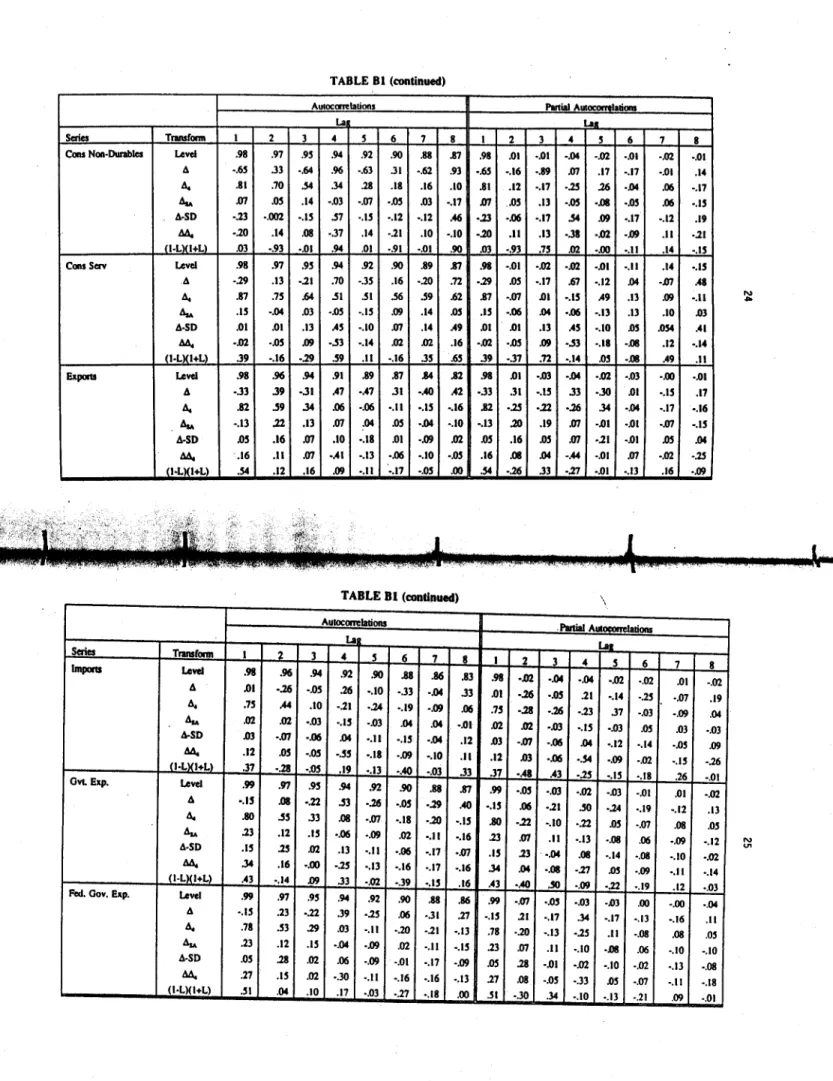
.86 .91 .38 -.18 .54 -.02 -.10 .82 :66 .• 37 . 06 \ , - ;41 ~.14 * All series 818 seasonally unadjusted except for the~ filter which rertes on seasonally

adjusted data

at

1he source. All series are in logarithms of the levels except for the change in business inventories, the unemployment rate, treasury bill rate, and ex post

real interest rate, which are in levels. · · ·

~~ ~ ~~ '

,s

corresponds to several transformations including judgemental corrections, aggregation across industries, time, etc.

Other transformations considered in Table 1 include a first difference with seasonal dummies, denoted A-SD, and a multiplicative M4 adjustment advanced by Box and Jenkins (1976). The former assumes a deterministic seasonal pattem, while the latter takes two unit roots at the zero frequency. 5

For the purposes of comparison, we also listed the AC function for the level of the series as well as the first difference where seasonals are ignored. Let us first discuss in detail the first series listed in Table 1, namely US GNP. The autocorrelation at lag 1 ranges from .98 to -.60 depending

on

which transfonnation (or lack of it) is considered . l, The .98 value comes, of course, from the level series but, even with A4, the removal of

the annual seasonal still leaves a very high autocorrelation at the first lag equal to .83. The · differences between the Census adjusted result of .37 and the common transformation A-SD (yielding -.02) suggests that transfonnations can have important effects on some of the time series properties of the data.

The differences in the patterns displayed in Table

t

for GNP are fairly representative for the other cases as well Consumption and M1 are just two of the examples appearing in Table 1 (additional details are also contained in the discussion paper version) .

What is clearly to be concluded,

as a

first impression from the results in Table 1, is that modelling seasonality, and the adjustment of data on the basis of such a model, seems to greatly affect whatever is left in univariate time series behavior-at lags other than the seasonal ones. The question which needs to be raised then is which data

5 The rransformalion wbicb consisls in eliminating die pair of 1001S (1-L) or {l-L)(J+L) conespondillg ta die biannual frcqueacy apparendy commoa in many maaocaJIIOlllic lime series (e.g1 Lee and Siklos (1991a. 19911:)

(6)

transfonnatlon appears most appropriate. For that, we tum to the Issue of testing for unit

roots

at the

seasonal frequency as each of the

data transformations considered treat 1his key feature differently.

3. The HEGY Procedure with P....a Data

BeNd

Model

Selectfon

In order to ascertain the presence of unit roots at the seasonal frequencies, as well as at the zero frequency,

we

follow the procedures outlined by HEGY, and

appried

by Beaulieu and Miron (1992), Engle, Granger, Hyllebefg and Lee (1992), Franses (1991), ·

lee and

Siklos (1991a),

Otto and

Wlrjanto (1991),

among

others. Moreover,

Ghysels, ~ · and Noh (1991) found the HEGY procedure compares fawrably with alternative'

procedures such as the Dickey, Hasza and Fuller (1984) tests, In tenns

of

finite

sample

size and power properties. In this_ section we Introduce the HEGY procedure. Since it~ ' ·,

, -i been widely documented elsewhere our cfiscusslon wlD be

brief.

Our main

focus

of

attention W11 Instead be directed towards extending the HEGY procedure to take accoui,ti of the fact one usually determines

the

order of the AR polynomial expansion

used

In

u;: ·

test on the basis of

the

data. The

fact

that the lag length

selection.

~'~:ba~h~S

something usually Ignored In theory but quite relevant and

Important

In

·pradlce>

~

µ'

dt

In

some

nontrivial distributional

Issues

regarding the

test

statistics.. Recently~

'.~o

.

work by Hall (1990) deals with data-based model selection In tests for unit

mots'

at"'iMi~

zero

frequency. We extend Hatrs results to that

of

HEGV procedures.

The

HEGY

approach consists In estimating the following regression:''.I>~''lfflf

d.t ", •

1t1 Yt.,-1 + Jrv'2.,-1 + ":JYJ,,-2 + 1t4)'3,,-J + ll +

P' D

1

(3.1)

+ • • • +

a

₁

A..x,-,

+

e,

where Jl Is a constant, & ls the slope coefficient of the linear trend, 01 is a vector

containing three deterministic seasonal dummies with coefficient vector

P,

(a1, ••• ,

ap)

are

the AR lag augmentations, and the Y14.'s (k=1.2,3) are series adjusted for unit roots at

other frequencies such that

Yu

Y21 =

=

Y:11

=

(1

+ L + L

2

_{+ L}

₃₎

_>,

- (1 • L + L2 -L

3)

xt

- {1 - L2)

xt

Thus. Ytt ls the series

xt,

after all seasonal unit roots have been removed. leaving only a unit root at the zero frequency. By contra~ Ya leaves a unit root at the bi-annual frequency for quarterly data so that (1+l) Ya is stationary; y31 then possesses a pair of complex roots

of

the annual frequency so that (1+L2) y31 ls stationary.

The test for the presence of unit roots Is based on the t-statistic for 1t1• for the zero frequency, "2 for the biannual frequency. For the annual frequency

we

require a joint test on "3 and _1t4,namely an F·test of the nun hypothesis

that Jta-""1f

4

=

O. Alternatively, the

t-statistic on ~· when 1t₄

=

0, may be used. Critical values for the tests were tabulated

by HEGY (1990), and the asymptotic distribution theory Is discussed in Engle, Granger,

(7)

A key assumption typically made both in the application of augmented

Dickey.

Fuller tests (henceforth

denoted

ACF) as well as the HEGY procedure is that the AR lag augmentation p Is known a priori. Yet. in many applications this assumption is

not

appropriate as researcher.s usually decide on the value of p on the basis of the available

data. Aa noted by Hal (1990), I Is clear that if p Is chosen using a data~sed model selection procedure, like tesmg which AR coefficients are significant

etc.,

then the ACF test, or the HEGY procedure, are actually.based on a pretest estimator.

Whether or not

the asymptotic distriJutlon of the ADF test changes, and for which model selection rules I doesn't, has also been studied by Hal. Drawing on his analysis and the resulls In

Ghysels, lee and Noh (1991) showing the correspondence

between

ADF and HEGYtest

will enable us to extend Hal's analysis to 1he HEGY procedure.

Consider

first the data generating process the HEGY procedure Is designed to test

z, •

J1o

+

cu,-4

+ JI, t • I, .... , T

where the error process has a AR<Po) representation, namely

,.

.., • E

'1

ll,-1 •

e,

J•I

(3.2)

(3.3)

The set-up In equations (3.2) and (3.3) portrays the data generating processes that go along with nun and alternative hn>olfleses of HEGY procedures. For simplicity, though·

not without loss of generality,

we

stripped away the time trend and seasonal dummies.· Hence with a= 1 In (3.2)

we

obtain a unit root all four frequencies of interest. In addition,"! the seasonal differenced process

~X.

follows an AR(Po) process which Is the raison •

d'Atre for discussing AR augmentation. In particular, let:

Assumption 3.1:

(1) The initial

vector

(Xe,,

x.

1, ••• ,

x-9o~

has a fixed distribution independent of (9t}.

(2) The roots of the characteristic equation of the AR(po) polynomial in (3.3) lie outside the unit circle.

(3) The

_sequence

of imovations (9t}

are

1.1.d. zero mean and constant variance

a1-

>

o.

The order p of the AR expansion in the HEGY equation (3.1) is selected by using a model selection procedure applied to the data. Namely, assume that p = ~ Is selected as the estimated value of

Po·

The estimated AR expansion has a well-defined probability distribution for any sample size T and

n~

=

D

represents the probability of obtaining an expansion of order

J,

where

J

= 0, 1, ... , J < -. Moreover, for any ~ =

J

we define

the

t-statistics; where i=1, ••• , 4 corresponding to the OLS estimates of 111 through it4 in the

HEGY equation (3.1). The following assumption will be key to the main result.

Assumption 3.2:

The model selection procedure satisfies the following conditions:

(1) as T-+oo, ~ - Po! O where! has a well defined probability distribution; (2) the distribution of~ Is independent of the distribution of the statistics; for i=1, ••.

, 4,

J=O •••

J and all T.

(3)

n~

<

Po)

=

0, I.e. the probability of underestimating

Po

Is zero as T -+-. The latter of the three conditions is important as it guarantees the convergence of the t-statlstics of the HEGY procedure to their distribution as characterized In Engle, Granger, Hylleberg and Lee (1992). Hence, under assumption 3.2 the

model selection rule leaves the test statistics unaffected. This is summarized in the following theorem, with the proof appearing in tha appendix to the paper.

(8)

Theorem 3.1:

Let assumption 3.1 and 3.2

hold.

then using ~ to detennine the AR lag expansion In the

OlS equation (3.1) yields the asymplotlc distributions:

'1J

=

fw1U>2 - 1)/2

[1·

W1(r)2drr2

"zJ

=

fw2(1}2 - 1)/2

[11

W2{r)2d,rl2 . fl [ fl 2 2

JIil

'3J

=

J>

(w3dw3 + w4dw4)/

J>

(w3(r)) + w4(r) )dr fl . .... .. · [ fl 2 2

JIil

t4J

=

J>

(w3uw4 + w4dw3)/

J>

((w3(r)) + (w4(r)) )dr

where

::$ denotes weak

c:onwrgence

In distribution, j

=

~ and w1(r), ("1=1,2,3,4), are

standard

Brownian

noUons on the uni Intervals (0, 1).

The proof of the theorem appears In the appendix. We should note that several

model selection criteria satisfy the assumption 3.2. Hall (1990) discusses several of them and analyzes their relative merls via a Monte

Carlo

Investigation. While several of the

criteria

yield more or less

smiler

l8SUlts Hars simulations

showed

a slight advantage Jo

)

using what Is known as a general-to-spec:ific model selectlon rule starting with some

upper bound on the length of the AR expansion. In the final analysis, the length of the AR expansion Is detennined by the longest statistically significant lag, where statistically significant means at

a

conventional signillcance level such as 5% or 10%. The application of this selection procedure oulperfonned the resort to selection criteria such as the

Hannan

and Quim criterion In particular. We conducted our empirical tests by utilizing the generat.t~ search procedure

as

well as the AIC and BIC criteria. Since there

was

liitle

differences

In the empirical results with the different criteria, and since the simulation

evidence In Hall tended to favor the general-to-specific rule, we will only report the empirical evidence with the latter in the following section.

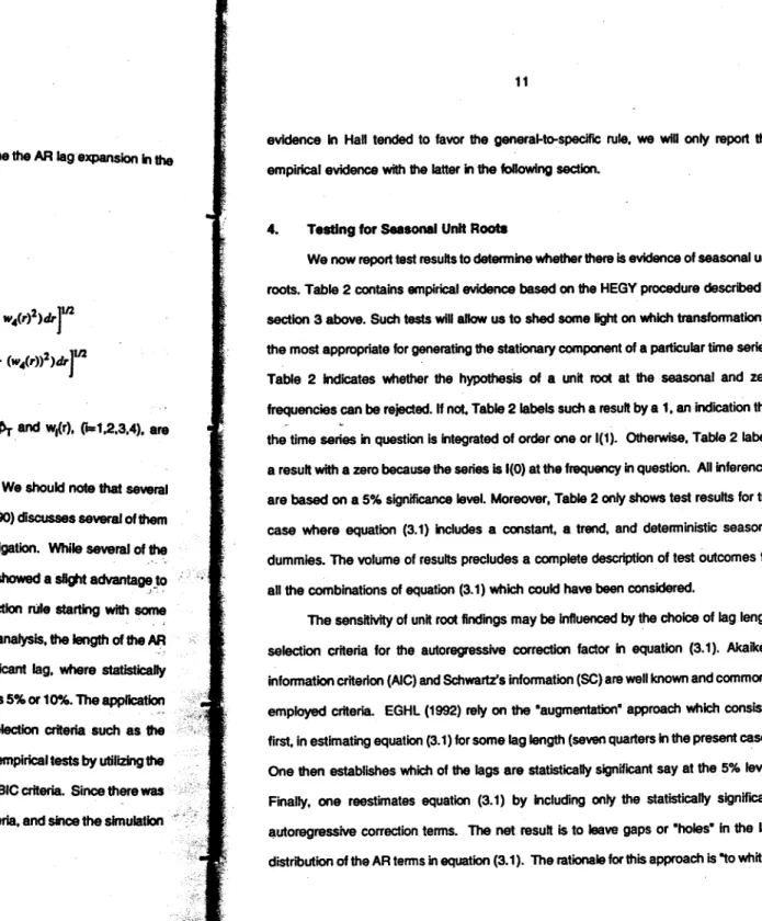
4. Testing for Seasonal Unit Roots

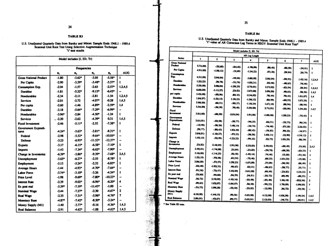
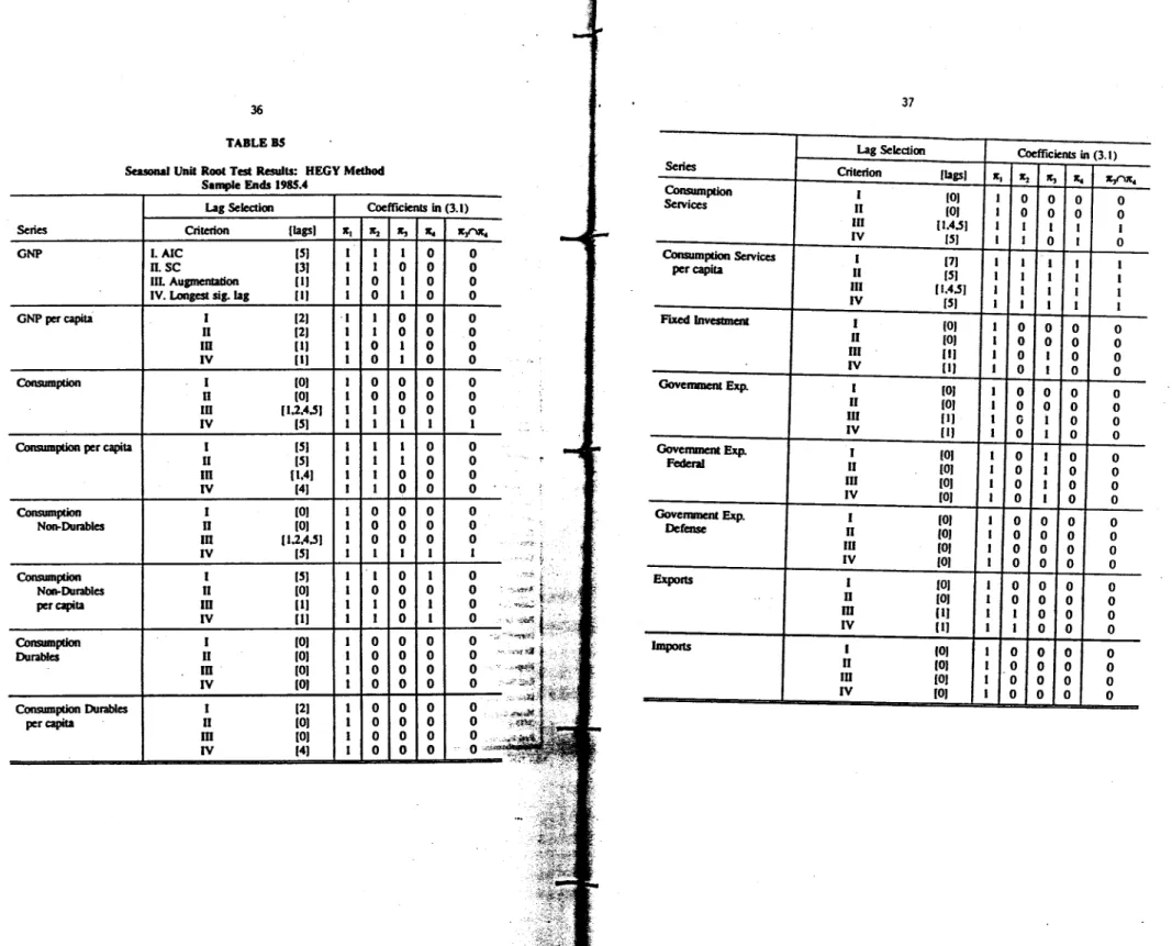
We now report test results to determine whether there is evidence of seasonal unit roots. Table 2 contains empirical evidence based on the HEGY procedure described in

section 3 above. Such tests will allow us to shed some light on which transformation is the most appropriate for generating the stationary component of a particular time series. Table 2 Indicates whether the hypothesis of a unit root at the seasonal and zero frequencies can be rejected. If not. Table 2 labels such a result by a 1, an indication that the time series in question is integrated of order one or 1(1). Otherwise, Table 2 labels a result with a zero because the series is 1(0) at the frequency in question. All inferences are based on a 5% significance level. Moreover, Table 2 only shows test results for the case where equation (3.1) includes a constant, a trend, and detenninistic seasonal dummies. The volume of results precludes a complete description of test outcomes for all the combinations of equation (3.1) which could have been considered.

The sensitivity of unit root findings may be influenced by the choice of lag length selection criteria for the autoregressive correction factor in equation (3.1 ). Akaike's information criterion (AIC) and Schwartz's information (SC) are well known and commonly employed criteria. EGHL (1992) rely on the •augmentation" approach which consists, first, in estimating equation (3.1) for some lag length (seven quarters in the present case). One then establishes which of the lags are statistically significant say at the 5% level. Finally, one reestimates equation (3.1) by including only the statistically significant autoregressive correction tenns. The net result is to leave gaps or "holes" in the lag distribution of the AR tenns in equation (3.1 ). The rationale for this approach is "to whiten

(9)

the residuals at the cost of the minimum number of parameters. Too many Pllrameters will decrease the power of the tests while too few will

render

the

size

far

greater than the level of significance.• (EGHL 1992). Based on Hall (1990), howew:tr, the preferred approach consists In estimating the number of AR tenns In equation (3.1) according to the longest lag with

a

statistically significant coefficient, beginning with a maximum

tag

length of 7 quarters. Below we report results using such a test procedwe, again

at

the ·

5%

level of

significance. To conserve space

we only present test results In

Table 2

based

on the general-to-specific selection path.

It should be noted,

however, that

the finding of an 1(1) or 1(0) was not generally sensitive, especlally

at

the

zan,

fraquency,

to the lag selection technique.8

Tuming

to

the results, It la apparent, especially from the last colultln of Table 2, that

very

few series

possess

a unit root at the

amual

frequency. The only exceptions are total consumption spending, consumption of non-durables, and the average real

wage:

These results reinforce the comparative difficulty of finding seasonal unit roots at the

,, ....

annual

frequency found by other researchers using

macroeconomic

data from other countries such

as

Canada

and

Japan (e.g., Lee and Sldos 1991, and EGHL 1992, ·

respectively). This

also means

that the M4 filter advocated

·-

'

6 _lbe_{--.,iu,oldil ,a:}_and_{riud . _ _}_being_pomble_ezc:q,tions._I.ee_ad_Still_(1991b)_Ibo

_{ladled_}

Ille - Cl1IIClmioa in tllcT C - -lmlple.

'l1lis

result is

inlenstiua

llecame 11111111 econmnlsts have fonliallled explamiona of businc&s c:ydc flllCIUllions 1llled on the ~ lhllt mlelllployment Ille Md GNP J1C1111*

cfifrt!mlf m , j ~ m,ie ..,.;e. ""1Pffllec fC.I! ·• ftf"'1C'llarrf MW! Oo:lh. f ~ l . C .• >

TABLE2

Seasonal Unit Root Test Results: HEGY Method1 Sample ends In 1989.4

Lag Selection

Coefficients

in (3. 1) Series Criterion (lags]

•,

_~Jr:,

••

lt;f\lt4

GNP longest Sig. lag (1) 1 1 1 0 0

Consumption (5) 1 1 1 0 1 Consumption (SJ 1 1 1 1 1 Non-Durables (OJ

.

1 0 0 0 0 Consumption Durables Consumption (5) 1 1 0 1 0 Services FIXed Investment (1) 0 0 0 0 0 Govemment Exp.

[1j

0 0 0 0 0

Government Exp. [OJ 1 0 1 0 0

Federal

Government Exp. [Of 1 0 0 0

6

Defense Exports (1) 1 0 0 0 0 Imports [OJ 1 0 0 0 0 Change In Bus. [5] 0 1 0 0 0 Inventories Employm8flt (1) 1 0 1 0 0 Unemployment (1) 0 0 1 0 0

Average Hours [OJ 1 0 1 0 0

Labor

Force

(1) 1 0 0 0 0

(10)

TABLE 2 (ConUnued)

Lag Selection Coefficients In (3.1)

Series Criterion [lags} _•1 _~_Ira

...

":f"lr4

Interest

Rate _(4J ₁ ₀ ₀ ₀ ₀

Ex post real _(OJ ₀

flterest rate 0 0 0 0

Average Wage ₍₂₁ ₁ ₀ ₁ ₀ ₀

Average Real ₍₇₎ ₁ ₀ ₁ ₁

1 Wage

Monetary Base _(Of ₁ ₀ ₀ ₀

0

Money Supply· M1 (1) 1 0 1 0 0

RealBalances · _[SJ ₁ ₀ ₀ ₀ ₀

1

_Based

_on_{estimates of}_{equation (3.1).}_{A constant,}_{trend, and}_{detenninistic}_seasonal

dummies are Included.

Signifies that the

test

result for the

s.

coefficient differed as

between

the seasonally

adjusted and unadjusted series.

by Box and Jenkins is generally unwarranted. The implication then is that, as in Osborn

(1990), Box and Jenkins type adjustments which ignore detenninistic seasonality can be mis-specifled.7 _{Moreover, since there are differences}_in_{the stochastic behaviour of} consumption _and income at the seasonal frequencies. These results may also have implications for the estimation and interpretation of consumption functions (see Lee and

Siklos 1991a).

There is, however, more evidence of roots on the unit circle at the biannual frequency. For total consumption, consumption of non-durables, consumption of services, the change in business inventories and GNP. If we restrict the analysis to the sample chosen by Barsky and Miron (1989) there is still more evidence of a seasonal unit root at the bi-annual frequency since for the labour force and wages series, one cannot reject the null that "2 = 0, in addition to the series found to have a bi-annual seasonal unit root for the extended sample. However, the foregoing exceptions to the finding of no seasonal unit roots at the bi-annual frequencies are interesting. For example, in the case of the

inventory series, the omission of stochastic seasonality may have implications for models which purport to show a link between inventory fluctuations and business cycles (e.g., see Ramey· 1989, and references therein). The finding of a seasonal unit root for the services · component of total consumption reveals the possible inportance of aggregation in estimating economic relationships such as the consumption function. Thus, the seasonal · unit root tests reveal potentially a considerable amount of mis-specification of seasonality

when only deterministic seasonality is assumed to exist.

This confirms not only the outcome of most unit root tests at the zero frequency, applied to

a

wide variety of U.S. seasonally adjusted macroeconomic data by several

7 Aa DOied previously, we conduc:ted all our tests with and without dclerminislic scasonaJs and omission of the lauer fealulc of the data influcna:s the conclusions rcadlcd ia Table 2.

(11)

researchers (see Campbel and Perron 1991 for a recent survey), but also reafllnns the neutrality of the X· 11 seasanal

a*5lmenf

procedure with respect to Its Impact on the existence of a unit root (see Lee and Sldos 1991 for Canadian evidence). One must,

therefore, conclude that while delenntllstic seasonal dummies capture much of the seasonal variation In the data there Is sulliclent evfcfenc» of the existence of seasonal unit

roolS to warrant the statement that 118 no seasonal unit root approach leads to

mis-specification of W1ivarlate time l8riea

behaviour.

This •1n between" result is probably

best

explained by arguments along the li1es of changing

seasonal patterns, see

Ghysets

(1991), and Canova and Ghysels (1992). Indeed. changes In seasonal pattems wiD not be captured by seasonal patterns

and

wll lead to spurious findings of roots at seasonal

frequencies.

5. Conclusion•

This

paper

has Investigated the properties of various filers appfl8d for the purposes of seasonal adjustment. Examination of aut~latlon and partial autocorrelation

functions

for widely used US quarterly macroeconomJc time series

suggests

conslderable differences

across

the various data transformations

considered.

We also extended Hairs work on the

Issue

of lag length selection In unit root

tests

to the unit root 1est Introduced by HEGY.

Toe empirical l'(tSults s ~ that, while seasonal dummies capture a great deal

of seasonal pattems. they do not seem to adequately describe an attnbutes. Indeed, unit

roots at some seasonal frequencies are regularly found. Moreover, none of the standard

transfonnatlons typically used to remove seasonais match the findings emel'(Jing from HEGY data-based model

selection

rules. One possible explanation for our findings Is that

seasonal

patterns change, only occasionafty though, as noted in Ghysels (1991)

and

\.}

Canova and Ghysels (1992). As such, none of the standard transformations suit this framework. Moreover, whatever transformation is applied seems to have a great impact on what is left as nonseasonal variation.

(12)

References

RB. Barsky and. J.A. Miron (1989), "The Seasonal Cycle and the Business Cycle,• Jcunal of Polltlcal Economy, 97 (June 1989), 503-34.

J.J. Beaulieu and JA Miron (1990), "Seasonal Unit Roots In Aggregate U.S. Data,•· Manuscript (Depattment of Ecouomics, Boston University).

W.R. Bel (1992), "On Some Properties of Linear Approximations to the X-11 Program," S1allstlcal Research Division, U.S. Bureau of the Census (mimeo).

W.R. Bel and S.C. Hilmer (1984), "Issues Involved with Seasonal Adjustment of Economic Tme Series," Journal of Business and Economic Statistics 2, 526-534.

O.J. Blanchard and D. Ouah (1989), "The Dynamic Effects of Aggregate Demand and

Aggregate Supply Disturbances,• American Economic Review, 79 (September 1989), 655-73.

· F.

Canova.

and E. Ghysels (1992), "01anges in Seasonal Patterns: Are They Cyclical?" Discussion Paper, Unlversil6 de Montr6al.

DA Dickey, W.R. Ben and R.B. Miller (1986), "Unit Roots in Time Serles Models: Tests

and Implications," The American Statistician 40, 12-26.

D.A. Dickey, D.P. Hasza and WA FuDer (1984), "Testing for Unit Roots in Seasonal Tme Series,• Journal of the American Statistical Association 79, 355-367. ,

R.F. Engle, C.W.J. Granger, S. Hylleberg, and B.S. Yoo (1990), "Seasonal Integration

and Cointegration," Journal of Econometrics, 44, 215-38.

P.H. Franses (1991), "A Multivariate Approach to Modeling Univariate Seasonal Tme

Series."

Econometric Institute Report No. 910/A.

E. Ghysels (1991), "On Seasonal Asymmetries and their Implications for Stochastic and Oetenninistic Models of Seasonality," manuscript, Universite de Montreal. E. Ghysels, H.S. Lee and J. Noh (1991 ), "Testing for Unit Roots in Seasonal Tme Series

- Some 1heoretical Extensions and a Monte Carlo Investigation," Oise. Paper, C.R.D.E. Universit6 de MontrmlL

E. Ghysels and P. Perron (1992), "The Effect of Seasonal Adjustment Fitters on Tests for . a Unit Root,• Journal of Econometrics (forthcoming).

C.W.J. Granger and P.L Siklos (1992), "Temporal Aggregation, Seasonal Adjustment,

and Cointegration: Theory and Evidence•, manuscript, Wilfrid Laurler University.

A. Han (1990), "Testing for a Unit Root in Tme Series with Pretest Data Based Model Selection," Discussion Paper, Dept. of Economics, N.C.S.U.

LP. Hansen and T.J. Sargent (1992), "Seasonality and Approximation Errors In Rational Expectations Models,• Journal of Econometrics (forthcoming).

S. Hylleberg, C. Jorgensen, and N.K Sorensen (1992), "Aggregation and Seasonal Unit Roots: A Note," Institute of Economics, University of Aarhus (mimeo).

S. Hylleberg, R.F. Engle, C.W.J. Granger, and H.S. Lee (1992), •seasonal Cointegration: The Japanese Consumption Function," Journal of Econometrics (forthcoming).

S. Hylleberg (1986), Seasonality In Regressfon, (Academic Press, New York.) H.S. Lee and P.L. Siklos (1991a), "Unit Roots and Seasonal Unit Roots in

Macroeconomic Time Series: Canadian Evidence." Economics Letters, 35,

273-77.

.

H.S. Lee and P.L Siklos (1991b), "The Influence of Seasonal Adjustment on Unit Roots and Cointegration: Canadian Consumption Function, 1947-91, • manuscript, Wilfrid Laurler University.

H.S. Lee and P.L Siklos (1991c), "The Seasonal Cycle and the Business Cycle: Money-Income Correlations in U.S. Data Revisited,• manuscript, Wilfrid Laurier University. C. Nelson and H. Kang (1981), "Spurious Periodicity in Inappropriately Detrended Time

Series," Econometrica, 49, 741-57.

M. Nerlove et al. {1979), Analysis of Economic Time Serles· A Synthesis (Academic Press, New York).

D.R. Osborn (1990), "A Survey of Seasonality in UK Macroeconomic Variables•, International Journal of Forecasting, 6, 227-36.

D. Otto and T. Wirjanto (1991), "Dynamic Adjustment of the Demand for Money for Canada," working paper no. 9114, University of Waterloo.

V.A. Ramey (1989), "Inventories as Factors of Production and Economic Fluctuations," American Economic Revfew, 79 (June), 338-54.

C.A. Sims (1974), "Seasonality in Regression", Journal of the American Statlstlcal Association, 69, 618-26.

C.A. Sims (1985). "Comment on 'Issues Involved with the Seasonal Adjustment of Economic Time Series' by William R. Bell and Steven C. Hillmer." Journal of Business and Economic Statistics, 3 (January), 92-4.

(13)

C.A. Sans (1992), ·Rational Expectations Modeling with Seasonally Adjusted Data,• Journal of Econometrics (forthcoming).

K.F. Wallis (1974),

•Seasonal

Adjustment and Relations

Between

Variables,• Journal of

the American

Weal

Aaoc:latlon, 69, 18-32.

•

APPENDIX

Proof of Theorem 3.1 Proof of Theorem 3.1:

We concentrate our proof on the case of t11 as the arguments for

'21

through t.c, are similar. Ghysels, Lee and Noh {1991), henceforth denoted GLN (1991), show there is

a

finite sample as well as an asymptotic equivalence between the HEGY t11 statistic, for

fixed and finite

J,

and the ADF t-statistic with a (j + 3) AR polynomial expansion. To discuss the equivalence we shal first make abstraction of the fact that a trend and seasonal dummies appear in ~uation (3.1). Consider, first, the DGP as descnbecl by

(3.2) and (3.3). Then GLN show that the regression equation

t.x, •

+1

x,-1

+ ~l.xr-1 + ~l.x,-2 +

+,1.x,_3

+ JI,

where

+

1 = a -1, while

ti

= -a for I = 2, •• , 4, yields at statistic for

+

1 whose f111ite sample and asymptotic distribution is the same as that of the HEGY t10 test. ·Naturally, this

equation corresponds to that of an ADF regression with an AR(3) expansion. This equivalence can be extended to HEGY procedures with j AR lags for

i

= 1, ..•• J < -. and also to HEGY procedures which include a trend and/or seasonal dummies. In the latter case, as Dickey, BeU and Miller (1986) show, one consults the OF distribution for a test statistic with a constant in the ADF regression equation. With this correspondence between HEGY ; and ADF with a (j + 3) expansion being established we can rely on the theoretical results in Hall (1990&. b). In particular, assumption 2.2 still holds with the transformation showing the equivalence between HEGY and ADF, namely (1)

(Pr+

3) -(Po + 3) :

o.

(2) the cf1Stribution of

Pr

+ 3 is stiU independent of the t statistic and (3)

nci>r

+ 3 <Po+ 3) = 0 also holds. Then applying theorem 2.1 and corollary 2.1 in Hall (1990) yields the result for the t₁₁statistic. An argument similar

in

nature also apply to the test statistics

'21

through t.c,, see GLN (1991) for further discussion.

(14)

Series Transform I 2 ONP Level .98 .96 4 • .6() .34 4, .83 .54 4._. .37

·"

4-SD •• ()'l • .003 44, .32 .12 11-Llll+LI .16 -.70 Cons. Level .98 .97 4 •.68 .41 A. .78 .6S 4._.

.o,

.22 4-SD -.41 .30 44, -.22 .13 11-Llll+Ll .07 •.85

Cons Durables Level .98 ;96

A ·.73 SI

,

A. .64 .38 I 4._. •.10 .IJ A-SD -22 .16 44, •.II .12 (1-L){l+L) .18 -.63

I

₀ '11 0

e

0

,,

Cl.

C:

s

TABLE Bl

Autocorrelations and Partial Auloc:ol'relatlon•

Autoconelalions

...

3 4 5 6 7 8 I .94 .92 .90 .89 Kl .85 .98 •.61 .90 ·.63 .32 ·.60 .66 •. fiO .22 •.06 •.18 •.16 ·111 .04 .83 .00 ·.10 ·.12 -.06 • .()2 •. 08 .37 -.15 .• 38 •.28 -.13 •.15 .31 ·.62 •.12 -.46 ·.36 •• 21 •.07

•. oo

.32 •.02 .72 ·.06 -.76 -.02 .f:11 .16 .95 .93 .92 .90 .88 .86 .98 •.67 .94 ·.6S .39 . .65 .91 •.68 .50 .32 .33 .30 .35 .38 .78 .04 -.OJ -.06 •. 12 .05 •.18 .05 .Jg .61 •• JO .19 ·.32 .54 ·.26 .OJ ·.43 .II •.21 .08 -.02 •.22 •.02 .89 .03 -.83 .01 .86

.rn

.94 .92 .90 .88 .86 .84 .98 •.72 .86 • .70 .52 ·.68 .83 •.73 .00 -.19 -.20 •. 21 -.13 -.02 .64 ·.11 •. 02 .03 -.06 -.04 -.16 •.10 -.20 .19 •.14 •. 02 •.09 .10 ·.22 •.01 -.42 .01 -.16 .01 -.01 •,II -.02 .59 -.03 -.65 -.02 .S9 .18 l'llrtial AIIIOCOnelalioos I • -2 3 4 5 6 • .()2 • .()2 _.;.01 _•.01 _·.00 -.05 ·.61. '. .71 •.27 •.23 • .44 -.26 •.04 .29 .()5 .13 -.15 •• 10 -.0'2 .03 • .1)()4 •.15 .38 •.34 •.12 .02. •.19 -.42 -.13 •.O'l •.74 .78 -.38 -.15 .IS •.01 ·.01 • .02 -.01 -.01 •.09 -.80 .69 .IS • .21

.II •.II •.17 .33 .OS

.22 .03 -.09 -.OS -.09 .23 •.32 .49 •.22 .16

m

.08 -.45 -.09 -.11 -.86 .74 .04 •.08 •. 10 -.0'2 •.02 .OJ -.02 •. 01 .09 •.60 .55 -.04 -.27 -.05 ·.23 -.26 .18 -.OS .12 -.09 •.06 .OS -.06 .12 -.IS .II -.OS -.12 .10 :01 -.4S -.10 -.08 -.68 ,56 -.07 -.22 -.21 7 •. 01 •. 11 •.08 .01 -.02 ·.06 .16 .06 •. 01 .14 .10 -.27 .03 .30 -.00 •. 12 .001 -.06 -.06 -.03 .24 8 ·.01 .II .01 ·.II .13 •.24 .06 -.01 .26 .002

.. u

.so

-.22 •.07 ·.01 .23 .003 -.16 .OS -.22 ·.04 N N

"'

...

(15)

TABLE Bl (continued)

Au1ocomlati011s

La

Serles Transronn I 2 3 4 5 6 7 8

Cons NClll•Dunblel Level .98 .97 .95 .94 .92 .90 .88 .87

A •,65 .33 •,64 .96 •,63 .31 •.62 .93 A. .81 .70 .54 .34 .28 .18 .16 .10 As.. ,07 .05 .14 ·.03 •,07 •,05 .03 •,17 .6-SD •,23 •,002

_··"

.57

.,.,

•,12 •,12 .46 64. •.20 .14 .08 •,37 .14 •,21 .10 •,10 ll•Llll+Ll .03 •,93 •,01 .94 .01 •,91 •,01 .90

Cons Serv Level .98 .97 .95 .94 .92 .90 .89 .87

.A • .29 .13 •.21 .70 -.35 .16 -.20 .72 A. .87 .75 .64 .51 .51 .56 .59 .62 As.. .15 -.04 .03 -.05 -.15 .09 .14 .05 A-SD .01 .01 .13 .45 •.10 .07 .14 .49 64. .,02 -.05 .o9 • .53 -.14 .02 ,02 _.16 (I.L)(l+Ll .39 -.16 • .29 .59 .II •,16 .35 .65 Exports Level .98 .96 .94 .91 .89 .87 .84 .82 A •.33 39 ·31 .47 •,47 31 • .40 .42 A. .82 .59 .34 .06 -.06 •,II •,15 -.16 As.. -.13 .22 .13 .07 .04 .05 • .04 -.10 A·SD .05 .16 .07 .10 •.18 .01 -.09 .02 64. ·.16 .II .07 • .41 -.13 -.06 -.10 -.05 ll•LKl+L\ .S4 .12 .16 .09

··"

-.17 -.05 .00 TABLE Bl (continued) Autocomlalions La Series Transronn I 2 3 4 5 6 7 8 lmpons _Level _.98 _.96 _.94 .92 .90 .88 .86 .83 A .01 ·.26 -.05 .26 • .10 -.33 -.04 33 A. .75 .44 .10 -.21 • .24 •.19 -.09 .06 As.. .02 .()2 _•.03 _-.15 _-.03 _.04 _.04 -.01

A-SD .o3 .,07 _·.06 _.04 _•,II _-.15

-.04 .12

64. .12 .05 -.05 -• .55 •.18 -.09 -.10 .It

ll•Llll+LI .37 •.28 •.05 .19 •.13 -.40 -.03 .33

Ovt. Exp. Level .99 .97 .95 .94 .92 .90 .88 .87

A •.15 .08 •.22 .53 ·.26 •.05 • .29 .40 A. .80 .55 .33 .08 -.07 •.18 ·.20 .,15 As.. .23 .12 .15 •,06 -.09 .02 •,II -.16 A-SD .15 .25 .02 .13 •,II •.06 -.17 •,07 64. .34 .16

•. oo

-.25 •,13 -.16 -.17 •,16 11-Llll+Ll .43 •,14 .o9 .33 -.02 -.39 •,15 .16

Fed. Oov. Exp. Level .99 .97 .95 .94 .92 .90 .88 .86

A •,15 .23 •,22 .39 •.25 .06 -31 .27 A. .78 .53 .29 .03 -.11 -.20 -.21 •,13 A,.. .23 .12 .15 -.04 .,09 _.02 _-.II _•.15 A-SD .05 .28 .02 .06 -.09 -.01 -.17 -.09 64. .27 .15 .02 •• JO -.ti -.16 •.16 -.13 (1-L)(l+L) .51 .04 .10 .17 •.03 -.27 •.18 .00 I 2 .98 .01 • .6.5 •,16 .81 .12

m

. .05 • .23 ·.06 ·.20 .II .03 •,93 .98 •.01 • .29 .05 .87 -.07 .15 -.06 .01 .01 .,02 _·.05 .39 .37 .98 .01 .33 .31 .82 • .25 -.13 .20 .05 .16 .16 .08 .S4 -.26 I 2 .98 .,02 .01 ·.26 .75 ·.28 .02 .02 .03 .,07 .12 .03 31 •,48 .99 •.05 •,15 .06 .80 -.22 .23 .07 .15 .23 .34 .04 .43 •,40 .99 -.07 -.15 .21 .78 ·.20 .23 .07 .05 .28 .27 .08 .51 -.30 Partial Alll""""'"lalions

_..

3 4 5 6 • .01 • .04 .,02 _·.01 •,89 ,07 _.17 •,17 •,17 • .25 .26 • .04 .13 •,05 ·.OS •,05 •,17 J4 ,09 •,17 .13 • .39 .,02 .J»

·"

.02 ·.00 •,II .,02 .,02 -.01 •.II •,17 .67 -.12 .04 .01 •,15 .49 .13 .04 ·.06 •,13 .13 .13 .45 •.10 .OS .09 • .53 •.18 -.OS .72 •.14 .05 ·.OS .,03 • .04 .,02 -.03 •,15 33 .30 .01 •.22 ·.26 .34 • .04 .19 .07 -.01 •.01 .05 .07 •.21 •.01 .04 -.44 -.01 .07 .33 .:r, •.01 -.13 \ .Partial A••-lalions La• 3 4 5 6 • .04 • .04 .,02 _•.02 ·.05 .21 •.14 -.25 •.26 •.23 31 -.03 ·.03 •.15 •.03 .05 -.06 .04 •.12 -.14 •.06 •.54 •,09 -.02 .43 -.25 -.15 -.18 •. OJ -.02 -.03 -.01 •.21 .50 • .24 •,19 -.10 -.22 .05 -.07 .II •.13 -.08 .06 . •,04 .08 •,14 •.08 •.08 .:r, .05 -.09 .50 -.09 •,22 -.19 •.05 •.03 -.03 .00 •,17 .34 -.17 •.13 -.13 -.25 .II •.08 .ti -.10 • .1)8 .06 -.01 •.02 -.10 -.02 -.05 -.33 .05 •.07 .34 -.10 •.13 •.21 7 •,02 •,01 .06 .06 •,12 .II .14 .14 -.0, ,09 .10 .OS4 .12 .49 -.00 •,15 •.17 .,07 .05 •,02 .16 7 .01 -.07 -.09 .03 -.05 -.15 .26 .01 •,12 .08 •.09 -.10 •,II .12 -.00 -.16 .08 -.10 •.13 -.11 .09 8 •,01 ,14 •,17

.,.,

.19 •.21 •,15 •,15 .48 -.II .03 .41 -.14 .II -.01 .17 •.16 -.15 .04 -.25 -.09 8 -.02 .19 .04 -.03 ,09 ·.26 -.01 -.02 .13 .05 •.12 -.02 •.14 •.03 •.04 .II .05 -.10 -.08 -.18 -.01 N

•

N u,

(16)

Au1ocorrelations La• Series Transronn I 2 3 4 5 6 7 8 I OvL Exp. 0ere11111 Level .99 .96 .94 .91 .88 .85 .82 .79 .99 A • .()4 _.47 _•,IS _.32 _•,27 _.21 _•,24 _.21 _•,04

A.

.80 .57 .38 .18 .06 .002 •.01 •.04 .80

As..

.65 .46 .34 .10 .01 0.06 •,08 •,02 .65 A-SD .II .37 .04 .18 •,13 J11 .,()IJ .03 .II AA. .35 .2A .04 •.25 •,19 •,12

•,04

·.03 .35 11-LVl+LI 64 .35 .26 .10 •,02 •,04 •,03 ·02 .64

Bm. Inv.

Chanae Level .67 .41

:n

•,OJ •,17 •,17 •.16 .,()IJ _.67

A .,09 •• J3 •,08 .23 •,08 _-.~7 •.05 .67 .,()IJ A. .62 .23 •,17 • .56 • .35 .,13 .10 .32 .62

As..

-.14 -.16 .21 _I -.23 -.17 -.OS -.06 -.02 -.14 A-SD -.07 •.52 -.06 .47 -.07 -.54 -.04 .75 -.07 AA. .01

_.o~

-.02 -.79 •,00 -.01 .02 .57 .01 /1,LVl+LI -.27 •.45 -.14 .17 -.48 .10 .65 .27 .27 F'axed Inv, Level .97 .92 .86 .82 .78 .75 .72 HJ .97 A • .30

.m

-.36 .84 -.38 -.10 -.36 .80 -.30 A. .78 .50 .22 -.03 -.14 -.19 -.19 -.18 .78

As..

.46 .18 .01 -.20 -.20 -.17 -.12 -.05 .46 A-SD .30 ,07 •,01 .17 -.07 -.15 -.05 .05 .30 AA. .41 .14 -.13 -.35 ·.28 -.15 .02 •,04 .41 0-L)(l+L) -.19 •.62 .03 .69 -.04 -.71 -.00 .65 .19 TABLE Bl (continued) AulOcomlalions La Series Transform I 2 3 4 5 6 7 8 Wages _Level _.98 _.95 _.93 _.91 .88 .86 .83 .80

A.

.96 .92 .87 .81 .77 .73 .68 .64

As..

.56 .36 .52 .70 .51 .27 .40 .54 A-SD .61 .46 .57 .68 .54 .36 .45 .52 AA. .II .16 .16 -.25 .04 -.07 -.03 •,06 /1,LVl+LI .80 .58 .67 .78 .64 .46 .52 .62

Real Wages Level .95 .90 .86 .81 .74 .68 .62 .57

A. .91 .79 .64 .45 .30 .16 .03 -.09

As..

.95 .90 .86 .81 .74 .68 .62 .57 A·SD .32 .22 .30 .36 .II -.02 .04 -.01 AA, .16 .19 .22 -.20 •.05 •,07 -.03 -.32 11-LVl+LI . 63 .27 .41 .47 .19 -.05 -.00 .07 Ml Level .98 .96 .94 .91 .89 .87 .84 .82 A .10 •.15 .01 .72 .02 -.16 -.05 .66

A.

.92 .80 .67 .56 .50 .46 .41 .37

As..

.57 .40 .30 .17 .29 .26 .09 .06 A-SD .~6 .16 .21

.so

.21 .10 .08 .41 AA. .31 .05 -.04 -.40 -.02 .05 -.14 -.06 (1-Llll+L) .98 •.08 .27 .66 .26 •,17 .18 .55 Partial Autocorreladons La• 2 3 4 J ₆ ₇ •,20 •,10 • .()4 •• ()IJ •,02 •. 01 .47 •,15 .13 •.21 .05 • .()4 •,19 •,04 •,17 ,09 ·.01 .05

.~

,02 • .24 •• 01 •,13 J11 .36 •.02 .05 •,18 ,02 .01 .14 •,10 • .31 .,02 ,09 .05 •,12 14 •,19 .01 •,OJ .06 .,06 .03 •.38 ,OJ .OJ ,09 ·.34 .,17 .10 •,13 •.37 .,25 • .24 • .34 -.47 .61 -.10 -.22 -.18 .17 •.22 -.18 •.23 -.10 -.53 -.21 .22 -.13 •.40 -.28 .03 .,02 _-.79 _•.01 _.13 _.01 • .57 .33 -.28 -.21 •.41

.ss

• .25 .02 .05 ,OI _.07 _-.01 -.17 . .49 .76 • .47 -.11 .07 • .25 -.19 -.13 .II •.07 -.03 • .()4 -111 -.22 •.01 -.05 •.03 -.03 -.02 .20 •.21 -.09 .07 • .()4 _-.21 _•.28 _-.01 _.01 _.03 -.68 .67 •.03 •,37 .,07 .22 Pal1ia1 Autoconelalions La• I 2 3 4 J 6. .98 -.01 -.02 -.02 -.03 •.01 .96 -.09 -.15 •,10 .20 •.08 .56 .07 .43 .47 .03 •.22 .61 .14 .39 .40 .03 -.20 .11 .15 .13 -.31 .06 •.01 .80 -.15 .73 -.13

.. os

-.16 .95 -.08 .02 •.OS •.21 •.02 .91 -.19 -.21 • .29 .II -.01 .95 -.08 .02 -.05 •.21 •.02 .32 .13 .22 .24 •.II -.17 .16 .17 .17 -.30 -.07 -.00 .63 •.21 .59 •,21 .,()IJ _-.26 .98 -.02 -.02 •,04 •,03 -.03 .10 -.16 '.04 .72 •.28 .03 .92 -.29 •,05 .02 .30 •,16 .57 .II .05 -.06 .27 .00 .36 .04 .16 .45 -.12 -.001 .31 -.05 •,04 -.41 .30 -.06 .48 •.40 .80 •.29 .02 ·.04 8 .00 .06 •,12 .OS .01 •• IJ •,02

.. oo

.50 -.18 •,II .51 -.18 -.09 •,02 .13 •.06 •.03 -.003 •,24 •,04 7 •.02 -.03 .03 .04 ,06 .21 .03 -.07 .03 -.06 .13 .07 •.02 •,02 •.10 -.21 ·.04 -.19 .31 8 •,02 -.07 .06 .03 -.17 .06 .04 -.18 .04 -.09 -.42 -.03 -.02 .30 .17 •.01 .26 -.18 -.23 ~ N ...

(17)

TABLE Bl (continued)

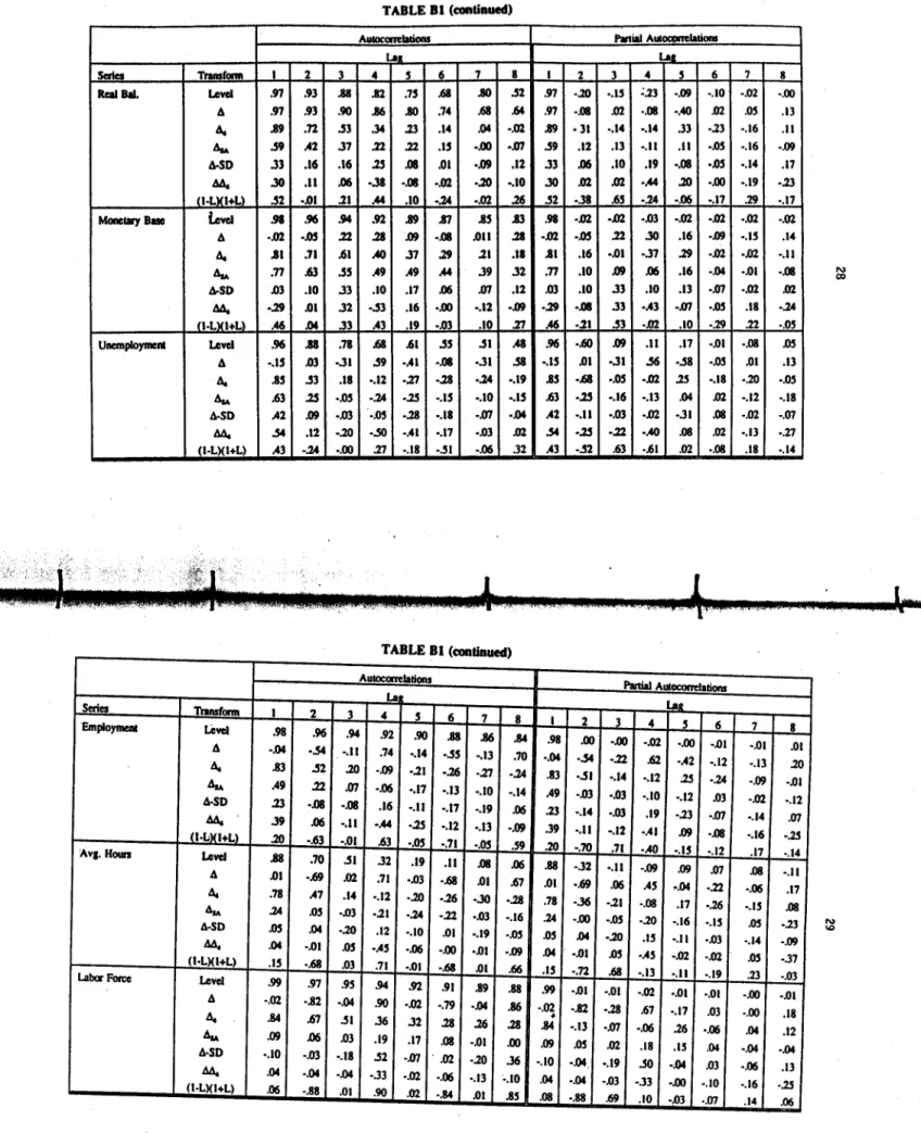
Auroconelalionl

LI•

c..a- TnMrl- I 2 3 ₄ ~ II 7 8 I

Real BIL Level .97 .93 .BB .82 .75 .68 .80 .52 .97

A .97 .93 .90 .86 .80 .74 .68 .64 .97

A.

.89

.n

.53 .34 .23 .14 .04 •,02 .89

~ .59 .42 J7 .22 .22 .15

• .oo

.m

.59

A-SD J3 .16 .16 .2S .OB .01 .11J .12 J3

AA.

.30 ,II .116 .JI ·.OB ·.02 ·.20 •,10 .30

fl•LVl+L) .52 -.Ol .21 .44 .10 • .24 -.02 .26 .52 Mane111y B•

i.cvel

.98 .96 .94 .92 .89 SI .85 .83 .98 A -.02 • .o., .22 .28 l1J -.08 .OIi .28 -.02

A.

.Bl .11 .61 .40 J7 .29 .21 .18 .Bl ~ .77 .63

.,,

.49 ,49 .44 J9 .32 .77 A-SD .03 .10 J3 .10 .17 .116

m

.12 .03

AA.

• .29 .01 J2 • .53 .16 -.00 -.12 .J» • .29 fl-LVl+U .46 .04 J3 .43 .19 -.03 .10

:n

.46 Unemptoymem Level .96 .BB .78 .68 .61 JS

.,,

.48 .96 A -.15 .G3 .JI .59 • .41 -.08 -JI

.,.

•,15

A.

.85 .53 .18 -.12 • .27 -.28 • .24 •.19 .85 ~ .63 .25 -.OS •,24 • .25 -.15 -.10 -.15 .63 A-SD .42 l1J -.03 •.05 -.28

....

.,(11 • .04 .42

AA.

.,..

.12 -.20 .JO •,41 •,17 •,03 .02

.,..

Cl·L)(l+L) .43 • .14 -.00 .27 -.18 -.51 -.06 .32 .43 TABLE Bl (continued) Autocomlalions La Serles _Transrorm _I ₂ 3 4 5 6 7 8 I Employment _Level _.98 _.96 .94 .92 .90 .BB .86 .84 .98 A •,04

_.,..

-.II .74 -.14 • .55 •,13 .70 -.04

A.

.83 .52 .20 •.09 •.21 -.26 • .27 • .24 .83 ~ .49 .22 .(11 •,06 •,17 •,13 -.10 -.14 .49

A-SD .23 ·.OS •.08 .16 •.II -.17 •.19 .06 .23

AA. J9 .06 •,II •,44 •.25 -.12 -.13 •,09 J9 tl,Llll+U _.20 _-.63 _-.01 _.63 _-.05

•,71 •,OS .S9 .20

Avg. Hours _Level _.BB

.70

.,,

J2 .19 .II .OB .06 .88

A .01 -.69 .02 .71 ·.03 ·.68 .01 .67 .01

A. .78 .47 .14 -.12 ·.20 -.26 .JO -.28 .78

As..

.14 .OS ·.03 •.21 • .24 •.22 -.03 -.16 .24 A-SD .OS .04 -.20 .12 •.10 .01 •,19 ·.OS .OS

AA. .04 ·.01 .OS •,4S •,06 •,00 ·.01 -.09 .04 (t.L)(l+L) .IS •,68 .03 ,71 •,01 •,68 .01 .66 .IS

Labor Force Level .99 .97 .9S .94 .92 .91 .89 .88 .99

A

•. oz

·.82 •,04 .90

• .oz

•,79 •.04 .86 •,02

•

A.

. 84 .67

.,,

J6 J2 .28 .26 .28 .84 ~ .09 .06 .03 .19 .17 .08 •,01 .00 .09 A-SD •.10 •,03 •.18 .52 .,(11 .. 02 •.20 .36 •.10 AA. .04 •.04 •.04 • .33 •.02 ·.06 •,13 ~.10 .04 O·L)(l+L) .06 -.88 .01 .90 .02 •,84 .01 .8S .08 Panill A111-lalion1 LI• 2 3 4 ~ 6 ·.20 •,15 ~.2.3 •I» •.10 ·.118 .02 •,08 •,40 .02 • 31 •,14 •,14 J3 .,23 .12 .13 •,II .II .,05 .116 .10 .19 ·.OB

. .o,

.02 .02 • .44 .20 -.00 •,38 .65 • .24 -.116 •,17 -.02 -.02 -.03 ·.02 ·.02 • .o., .22 .30 .16 .J» ,16 -.Ol -J7 .29

• .oz

.10 l1J .116 .16 -.04 .10 J3 .10 .13 •• (11 -.08 J3 • .43

_-m

-.05 .,21 .53 ·.02 .10 -.29 -.60 l1J .II .17 -.01 .Ol •JI .56 •.SB -.05 -.68

•. os

-.02 .25 •,18 -.2S -.16 -.13 .04 .02 •,II -.03 ·.02 -JI .08 • .25 •.22 • .40 .08 .02 .JZ .63 ·.61 .02 •. 08 Partial Autocorrelalions La• 2 3 4

s

6 .00 ·.00

•• oz

•,00 -.01

.

.,..

_•.22 _.62 _•,42 _•.12

_.,,

_•,14 _•,12 .25 • .24 -.03 ·.03 -.10 •,12 .03 •.14 •,03 .19 -.23 .,(11 •,II -.12 •,41 l1J ·.OS •,70 .71 • .40 •,IS •.12 •.32 •.II ·.09 .09

_m

-.69 .06 .45 •. 04 •.22 ·.36 ·.21 ·.08 .17 -.26 •,00 -.OS

• .zo

•,16 -.15 .04 ·.20 .IS •.II •.03 .•• 01 _.OS _•,4S _•,02

_{•. oz}

•,72 .68 •.13 •.II .,19 ·.01 -.01 •,02 •.01 •.01 •,82 ·.28 .67 ·.17 .03 -.13 .,(11 -.06 .26 •,06 .OS .02 .18 .1.5 .04 •.04. •.19

.so

-.04 .03 •.04 ·.03 ·J3 ·.00 •,10 ·.88 .69 .10 ·.03 • .(f1 7 •,02 .05 •,16 -.16 •,14 •.19 .29 -.02 •.15 ·.02 •. 01

•. oz

.18 .22 -.08 .01 •.20 -.12

•. oz

-.13 .18 7 -.01 •,13 •,09 -.02 -.14 •.16 .17 .08 -.06 •.IS .05 ·.14 .OS .23 •.00 •,00 .04 •,04 •.06 •.16 .14 8 •,00 .13 .II -.09 .17 • .23 •,17 •,02 .14 •,II -.118 .02 • .24 •.OS .OS .13 •.OS •,18 .,(11 •. 21 •.14 8 .01 .20 •,01 •,12

m

·.25 •.14 ·.II .17 .OS -.23 •.09 •.37 ·.03 •,01 .18 .12 •.04 .13 • .25 .06

"'

\Q

"'

00

(18)

Autoconelalions P1rtia1 Aulnmnll!lations

La Lao

Serio Transform I 2 1 4 5 6 7 8 I 2 1 4 5 6 7 8

Treasury bill Level .96 .91 .88 .84 .80 .76 .72 .70 .96 •,16 .22 •,17 .OS .,13

m

.21

A .04 .15 .05 .03 ·.01 .G2 •.33 .03 .04 •,15 .07 .00 .00 .G2 •,34 .09 A, .74 .48 .26 .,07 •,14 •,17 • .24 •,18 .74 •,17 .,07 •.42 .37 ·.20 •,07 •,04 ~ .17 ·.28 .08 ,06 ,06 .,04 _·.32 _·.01 _.17 _·.32 _.23 _•,13 _.21 •,20 •,22 .08 A-SD .96 .92 .88 .84 .80 .77 .73 .71 .96

·111

m

·.08 ·.01 .,02 _·.01 _.27

M..

.()2 •,09 . .20 • .49

.m

.10 ·.28 .01.

112

•,09 .21 • .54 ,06 _·.08 •,II •.27 l1°LVl+L\ .45 •,10 ·.01 .05 .01 •,15 • .29 .,07 .45 •,38 .32 • .24 .21 •,44 .15

.. os

El post real In&. Ille Level .713 .55 .50 .30 .23 ,17 .14 ,II .71

m

.16 ·.26 .08

•. os

.14 •,09 A .57 J7 .36 .28 .22 .19 .13 .ll .57 .0, .20 ·.00 .()2 ,02 _·.03 _.01

A, .25 .12 .20 • .24 ·.01 .01 •,12 •,ll .25 ,06 .17 • .37 .15 .,03 .01 .,25

~ • .25 .,23 JO .,20 _•.05 _.03 _.01 _•.18 .,25 .JJ .17 •.16 ·.03 •.15 .05 .,27 _~

A-SD • .33 •,19 .13 -.08 .,03

.io

.,07 .,02 • .33 • .33 .,07 •,15 •.12 .003 •,06 •,05

M. •.41 •,14 .34 •,45 .14 .II •,10 •.03 •,41 •,37 .16 • .36 .,14 .,15 .10 .,27 (1-L)(l+L) •• 01 • .36 .IS ,()() •,07 .,()() .00 .CTI ·.01 • .36 .16 •,16 .CTI -.11 .04 .04

CPI Level .98 .97 .95 .94 .92 .90 .89 .87 ,.98

• .o,

·.01 .,()() _-.01 _-.01 _{· -.01} _•,02

A .58 .40 .41 .32 .25 .23 .16 .12 .58 .10 .22 •,00 .G2 .02 •,OS .00 A, .90 .77 ,(iS .54 .44 .35 .26 .20 .90 • .23 ,04 -.07 .02 •.09 -.01 .04 ~ .78 .66 .13 A6 .39 .34 .28 .21 .78 .13 .20 -.27 .08 -.03 .10 -.13 A-SD .60 .43 .41 .31 :J.1 .26 .16 .10 .60 .12 .18 •,04 ,06 .04 -.09 ·-.03 M. .31 .IS :J.O -.21 -.01 .01 -.13 -.13 .31

m

.15 -.36 .16 -.03 -.02 .,25 (1,L)(l+L) .80 .56 .48 .41 .33 .27 .21 .15 .80 -.26 .38 -.26 .23 -.20 .12 •,15 • AD series are seasonaUr unadjusted except for the A.,. filter which ielies oo seasonally adjusted clala 11 lhe source. AD series are in loprilhms of the levels except for

lhe change in business mvenlllries, lhe unemployment Ille, trusury bill raie, and ex post iuJ inieiest raie, which m in levels.