Design evaluation and optimization for models of hepatitis C viral dynamics

HBV DNA detection and quantification is useful in clinical practice to: (i) to diagnose chronic hepatitis B with viral replication; (ii) establish the prognosis of liver disease and

Keywords ICMS, excitable-tissue model, ion-channel subtypes functional role, nonlinear dy- namics, meta-parameter, bifurcation analysis, mixture model, energy for neural

Considering the current knowledge, this is the first time a method trained on simulated data is successfully used on real data for (binaural) sound source localization, validating

Using the surrogate model in an evolutionary op- timization algorithm, the adaptive sampling decisions change from selecting which points of the input space to evaluate in order

Viral escape from antibody-mediated neutralization in these individuals may occur on several levels: (i) HCV exists as a quasispecies with distinct viral variants in

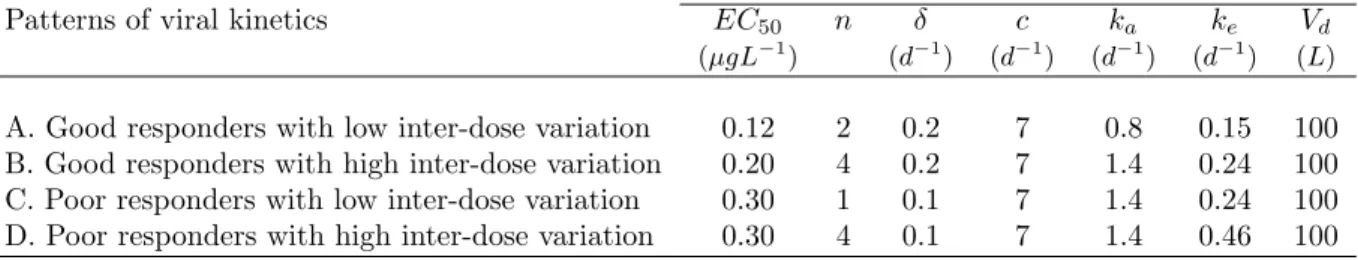
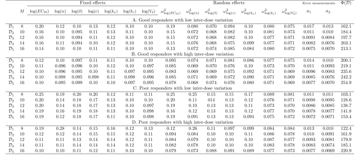
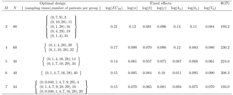
We define an elementary design as a set of sampling times.. A nonlinear mixed effects multiple response model or a multiple response population model.. is defined as follows.

Indeed, as shown in Table 1, although many sensitive innovative and miniaturized sensing mechanisms have been developed for the diagnosis of viral hepatitis, very few

η =0°.. Figure 6.16: Stage attachment angle, η, effect on the serial spider concept subsystem stiffness ratios. The ratios are normalized using the corresponding ratio value for