NAMB: A Quick and Flexible Stream Processing Application Prototype Generator

HAL Id: hal-02483008

https://hal.archives-ouvertes.fr/hal-02483008

Submitted on 18 Feb 2020

HAL is a multi-disciplinary open access

archive for the deposit and dissemination of

sci-entific research documents, whether they are

pub-lished or not. The documents may come from

teaching and research institutions in France or

abroad, or from public or private research centers.

L’archive ouverte pluridisciplinaire HAL, est

destinée au dépôt et à la diffusion de documents

scientifiques de niveau recherche, publiés ou non,

émanant des établissements d’enseignement et de

recherche français ou étrangers, des laboratoires

publics ou privés.

NAMB: A Quick and Flexible Stream Processing

Application Prototype Generator

Alessio Pagliari, Fabrice Huet, Guillaume Urvoy-Keller

To cite this version:

Alessio Pagliari, Fabrice Huet, Guillaume Urvoy-Keller. NAMB: A Quick and Flexible Stream

Pro-cessing Application Prototype Generator. The 20th IEEE/ACM International Symposium on Cluster,

Cloud and Internet Computing, May 2020, Melbourne, Australia. �hal-02483008�

NAMB: A Quick and Flexible Stream Processing

Application Prototype Generator

Alessio Pagliari, Fabrice Huet, Guillaume Urvoy-Keller

{alessio.pagliari, fabrice.huet, guillaume.urvoy-keller}@univ-cotedazur.fr

Abstract—The importance of Big Data is nowadays established, both in industry and research fields, especially stream processing for its capability to analyze continuous data streams and provide statistics in real-time. Several data stream processing (DSP) platforms exist like the Storm, Flink, Spark Streaming and Heron Apache projects, or industrial products such as Google MillWheel. Usually, each platform is tested and analyzed using either specifically crafted benchmarks or realistic applications. Unfortunately, these applications are only briefly described and their source code is generally not available. Hence, making quick evaluations often involves rewriting complete applications on different platforms. The lack of a generic prototype application also makes it difficult for a developer to quickly evaluate the impact of some design choices.

To address these issues, we present NAMB (Not only A Micro-Benchmark), a generic application prototype generator for DSP platforms. Given a high-level description of a stream processing application and its workload, NAMB automatically generates the code for different platforms. It features a flexible architecture which makes it easy to support new platforms. We demonstrate the benefits of our proposal to quickly generate application prototypes as well as benchmarks used in published papers. Overall, our approach provides easily replicable, comparable and customizable prototypes for data stream platforms. Moreover, NAMB provides similar performance in terms of latency and throughput to existing benchmarks, while only requiring a simple high-level description.

Index Terms—Application Generation, Application Prototype, High-Level description, Data Stream Processing

I. INTRODUCTION

New trends in Big Data require to process high-rate un-bounded data flows in almost real-time. Data Stream Process-ing (DSP) is a popular approach to deal with this constraint in many fields, from social networks to IoT. As most ap-plications need to manage sensible data and require a high level of responsiveness, the continuous flow of incoming data needs to be processed in a quick and correct manner. Many platforms have been developed to tackle the problem, such as the Flink [1], Storm [2], Heron [3] Apache projects or the Spark Streaming [4] extension, as well as industrial solutions such as Google Millwheel [5]. All of them propose different approaches and architectures to address the same challenge, namely optimizing the stream processing performances by assuring reliability, high throughput and low latency among other features.

To analyze different platforms or test topology designs, it is necessary to use a variety of test applications. However, writing several applications to encompass all the possible

implementation designs may be costly and time-consuming. Current works commonly use test applications as benchmarks or mocks of production applications. Most of the available test applications tend to be bounded to the platform or scenario they are evaluated on. As a consequence, it makes those applications hardly usable in other contexts. Moreover, this ad-hoc approach does not always allow an easy tuning of the application. Indeed, even some slight changes of the application characteristics require modification of the source code. This becomes a limitation when the source is not available, or when the application internals are not correctly explained. Thus, a reference solution is missing. We feel the necessity for a flexible and generic approach that is context-and platform-agnostic. That would allow to easily configure the fundamental DSP applications characteristics, together with a detailed workload description.

In this paper, we present Not only A Micro-Benchmark (NAMB), a framework that, given a generic application model, will automatically generate the defined application. It builds over our previous work where we introduced the idea of a generic high-level model to describe DSP applications [6]. NAMB is based over fundamental data stream characteristics and supports an easy and quickly configurable topology de-scription. Based on this description, it can generate code for various platforms. Thanks to its high-level definition schema, NAMB allows for an easy and quick generation of a large set of micro-benchmarks as well as prototypes of realistic applications.

Our contributions are as follows:

• Based on a detailed analysis of the fundamental char-acteristics of DSP applications, we propose a high-level model to precisely describe each element of a typical application.

• We propose NAMB, a platform for fast and flexible

generation of prototype applications based on their high-level description.

• Additionally to an internal synthetic generation, we in-clude the support to connect NAMB to an external Kafka cluster.

• We demonstrate how NAMB can be used to evaluate the

impact of design choices and create complex prototypes to analyze DSP systems, only by using high-level models instead of editing the application code.

• We make available a public release of NAMB at https: //github.com/ale93p/namb, ready for Storm, Flink and

Heron.

II. RELATEDWORK

Our objective is to create application prototypes that would help to run different kinds of tests on DSP systems. We firstly analyze representative applications used in literature to evaluate DSP systems, such as benchmarking applications. Secondly, we consider the proposed solutions for application generation.

A. Benchmark Applications

The first benchmark application appositely developed to benchmark streaming data is Linear Road [7]. The authors define implementation guidelines for a benchmarking appli-cation. Their proposal simulates a real scenario: an urban expressway system. Its objective is to monitor real-time traffic to adapt the tolling price to the road congestion.

Currently, the most popular benchmark application is the Yahoo! Streaming Benchmark [8]. The application (Fig. 1) analyzes advertisement interactions on the Web. The data reaches the application as an stream of events from Kafka. They are deserialized and parsed into different fields, keeping only the ad view events. They are then assigned to a campaign id from a Redis database. Finally, events are counted by campaign id. The Yahoo! Benchmark has been widely used by companies to evaluate their solutions [9], [10], [11]. It has been implemented for Storm, Flink and Spark Streaming.

Fig. 1: Yahoo Streaming Benchmark Design [8] Yahoo! also presented two other typical industrial topologies in [12]: PageLoad and Processing. They are used to manage real-time advertisement events. Both are presented as a set of standard queries without any details regarding the actual workload.

In StreamBench [13], the authors define a set of workloads, characterizing them in terms of data type and computational complexity. They then propose 7 different benchmark applica-tions representing those scenarios. The applicaapplica-tions are tested with two different real-world data sets (textual and numeric). BigDataBench [14] is devised for both batch and streaming platforms with a focus on Internet services. BigDataBench is composed of a large set of applications, each related to a specific Internet service, such as: Search Engine, Social Network, E-Commerce, Bioinformatics and Multimedia Pro-cessing. JStorm[15] and Spark Streaming[4] are currently supported.

The authors in [16] propose RIoTBench, a suite designed specifically for IoT. They analyze the characteristics and the behavior of common applications in this context, describing common task patterns used in streaming applications for IoT. The suite regroups a large set of IoT micro-benchmarks as well as a set of representative IoT applications, to cover all these patterns.

In [17] the WordCount standard application is presented. It is commonly implemented as a test and example application by the various stream processors. In addition, the authors introduced two applications with real datasets: an air quality monitoring application and a flight delay analysis.

When an application is developed for benchmarking it is commonly designed with a specific objective in mind, such as evaluating specific metrics or particular platform mech-anism. They are limited by a static compositions of tasks, other than by the platform-specific implementation. Although most of these applications are representative of real industrial workflows or they replicate common DSP queries, they may not match the user-specific environmental needs. This lack of flexibility and generality does not allow customized workflow compositions or an easy cross-platform evaluation.

B. High-Level Models and Generation

Several higher-level languages for DSP [18] have been proposed. The main objective is to introduce mechanisms or concepts previously not supported, or optimize the application generation.

Apache Beam [19], [20] tries to enclose all the key mech-anisms that a DSP system should support, through a common set of Java APIs for the different streaming platforms. A particular attention is paid to the windowing mechanism, and a new model for windowing is proposed. It can support out-of-order data arrivals along with session windowing. Then, Beam Runnerstranslate the Beam APIs into platform-specific code, allowing cross-platform development and ensuring a common set of functions between all of them.

SECRET [21] defines a general semantic do describe the different Stream Processing Engines (SPEs) mechanisms. The framework aims to compare and ease the understanding of SPEs internal behaviors, which are normally differently im-plemented. In their paper, the authors mainly focus on the windowing mechanism implementing a framework aimed to continuously monitor the window status of the application.

The authors of SpinStreams [22] present a framework to optimize the tasks implementation in DSP applications. Given a topology description in xml and the java functions to describe the tasks workload, SpinStreams applies operators fission (task replication) and fusion (merging two or more tasks into a single one) to optimize the query executions and improve application performances.

Another example of query language for DSP is Piglet [23], an extension to Pig Latin [24] directed to Stream Process-ing functions. Given an high-level description of the stream processing queries, Piglet generates application code for the different SPEs. They define a SQL-based API to write the

application that generalizes the supported platforms features. Similarly to SpinStreams, they rewrite the application code to optimize the query execution.

The above works propose high-level description models to define DSP topologies. They expose programming languages APIs to write the code, or require actual code for user-defined functions. The main objective is to generate executable application code for the different SPEs. At the same time, they focus on optimizing the query planning or introducing and generalize missing DSP features to these engines.

Our work goes on a different direction. We aim to generate prototype applications, with a simulated workload, i.e., we don’t require the user to specify the internal code of each task. This approach would allow a quick and easy definition of the topology graph, without the need of writing the application code, through an high-level and simple description of the workflow [6].

III. MOTIVATION ANDCHALLENGES

We just showed that the literature already provides us with a large variety of streaming applications and application generators. However, we think that this past work presents various limitations:

• Context-Specific: those applications are commonly

de-signed for specific platforms or specific scenarios such as IoT or Internet services, limiting their applicability to other fields of study.

• Code-Bounded: applications and generators require to write actual code. As already pointed out, this can be time-consuming, especially for quick evaluations.

• Complex Reproducibility: most applications, especially micro-benchmarks, do not specify the kind of workload that is implemented. They usually define a general ob-jective of the evaluation – e.g. I/O intensive, maximal throughput – without a detailed definition of the tasks internals, making most of the times the evaluation not reproducible;

• Static Nature: an imprecise description of the pipeline

and hard-coded configurations do not allow a quick and easy tuning of the applications proposed in the literature, preventing an easy study of different implementation choices;

• Unavailability: Last but not least, the software presented in the literature are often not publicly available.

These drawbacks point to a lack of an easy-to-design and generic solution, that could be used in every context and that could be quickly adapted to the underlying environment. For such reasons, we think it is necessary to have a prototype application generator that could address those limitations, i.e. that is: (i) generic: able to run on or be adapted to any kind of streaming platform or environment, so as to support current and future data stream frameworks and features; (ii) flexible: with a well defined description model of the workflow, that can be quickly and easily customized; (iii) available: as open-source, so as to be ready-to-used and continuously improved by the community.

To achieve these objectives, we need an initial description and model of a typical data stream application. Thus, we first define several fundamental characteristics common to DSP ap-plications (Section IV), which have a significant impact on the characterization of an application workload. We then abstract these characteristics in a set of parameters configurable by the user through a high-level set of configurations (Section V). Finally, we implement a framework that, given this model, will automatically generate the application to be deployed (Section VI).

IV. FUNDAMENTALCHARACTERISTICS

Streaming applications are composed by a pipeline of tasks that continuously process data flowing into the application. For this reason we divide DSP applications fundamental characteristics into two categories: data stream and workflow. The former defines the input stream of the application. The latter describes how the data is transferred between tasks and how it is processed. The two categories are interdependent as the workflow is impacted by the characteristics of the data stream.

A. Data Stream

a) Data Characteristics: Data variety is a base char-acteristic of Big Data. Data can be of various types, from text to binary, as well as of different size depending on the application.

b) Input Rate: Data may arrive at different rates and following different distributions, from simple Constant Bit Rate (CBR), to bursty traffic.

B. Workflow

a) Connection: A DSP application is logically repre-sented as a Directed Acyclic Graph (DAG) starting with sources and ending with sinks. The DAG can assume various forms based on the application pipeline.

b) Scalability: Streaming systems are designed to man-age high loads of data. Most components of the topology can be parallelized to spread the incoming load over multiple instances.

c) Traffic Balancing: Data needs to be routed through the different task instances. The various streaming platform usually implement standard grouping methods, e.g. round-robin or key-based.

d) Dependency: A task may need to combine data from more than one incoming path, like in the case of Complex Event Processing [16]. This requires to keep data stored until the complementary tuple arrives.

e) Message Reliability: To ensure message processing, some DSP platforms offer reliability mechanisms. Those may impact the application performance [25].

f) Windowing: An important characteristic of a contin-uous stream of data is its endlessness. For this reason, most applications try to give partial results over time periods. This continuous method of aggregation is implemented through a windowing system.

g) Data variability: As stated before, the input data stream can be described by type, size and distribution. How-ever, during the stream processing, some tasks may alter the data, e.g. through filtering, projections, etc. Hence, the characteristics of the dataset may change on the fly.

h) Workload: The different tasks in the pipeline perform different operations on data. Some are more computationally intensive than others.

i) I/O Operations: A common task in data processing is the interaction with an external database (read or write). These operations will consume time and resources and thus add an external factor influencing performance.

We have described the properties that directly impact the deployment and performance of streaming applications. We used these characteristics to design our generalized model, in the next section, for the prototyping workflows.

V. HIGH-LEVELDESCRIPTION

We defined a generic schema for a coarse-grained descrip-tion of the global behavior of the applicadescrip-tion, called the Workflow schema [6]. To that first schema, we juxtapose a second one closer to a real application definition, named the Pipeline schema. The latter allows the user to specify the exact DAG they want to evaluate, with parameters for each task. These two approaches make it possible to easily and quickly define prototype applications, but also describe large and complex mock applications.

Both models follow the YAML standard [26] for their configuration files, which will serve as input to the generator (Section VI). It thus consists of a series of key-value pairs grouped into different blocks.

A. Workflow schema

The Workflow schema is the base general description of the application characteristics. We derived it directly from the fundamental characteristics described in Section IV [6]. This schema enables the user to quickly and easily define, customize and generate simple application prototypes. This allows to swiftly tune some application features (e.g. level of parallelism, computing load, topology shape), to easily experiment different design combinations.

B. Pipeline schema

Differently from the Workflow schema, the Pipeline schema doesn’t describe the topology from a generic point of view. It focuses on the description of each tasks and connections to accurately define more specific characteristics. Similarly to what a user would write to build a real application using platform-specific APIs. The main advantage of this schema is that it allows to tune the parameters at task level, giving more freedom to shape the application.

The configuration file consists of a main section to describe the pipeline of tasks. A task can either be a source or a processing unit, depending on the properties used to configure it. The data stream is described directly in the source task, defining how that specific task will generate data, or if it is connected to an external source (Section VI-D2).

The user can also specify different sources with a specific behavior each. Meanwhile, the workflow is defined at a per-task level. Each per-task is defined by its own properties, as processing workload and parallelism. Each task will define the parent tasks and how they are connected to the previous level in the DAG. This allow to create more complex topologies that do not strictly match one of the layouts provided in the workflow schema.

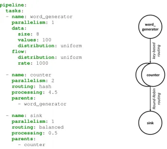
Fig. 2 shows an example of a configuration file with the associated topology for the Pipeline schema. A source (word generator) will send data at a rate of 1000 tuples per second to 2 counter tasks using a hash-based routing. To simulate a real processing load (Section VII-C), we use here a busy-wait loop of 4500 cycles (4.5 in the configuration file as the unit is a thousand of cycles). Finally, the data is sent to a sink, which will perform some light processing.

pipeline: tasks: - name: word_generator parallelism: 1 data: size: 8 values: 100 distribution: uniform flow: distribution: uniform rate: 1000 - name: counter parallelism: 2 routing: hash processing: 4.5 parents: - word_generator - name: sink parallelism: 1 routing: balanced processing: 0.5 parents: - counter word_ generator sink counter ke y-base d ro ut in g Ro un d-Ro bi n ro ut in g

Fig. 2: Per-task configuration with the Pipeline schema (yamb.yml)

VI. NOT ONLYA MICRO-BENCHMARK

In this section we present the details of NAMB – Not only A Micro-Benchmark. Given a high-level definition of the workflow for the Workflow schema or the Pipeline schema, NAMB automatically generates the corresponding application for multiple platforms.

A. NAMB Design

Once the user has written her high-level YAML model, NAMB is executed through a main command line script, through which the user is able to specify for which platform the application will be generated. The script will create and deploy the generated application on the platform of choice.

NAMB core is composed by three main components (Fig. 3). The Application Builder that takes the input con-figuration and reads the defined parameters; the Topology Generator that, based on the specified platform, will trans-late those configurations into platform-specific code; and the

LoadGen KAFKA CONSUMER SYNTHETIC GENERATOR DATA GENERATION FLINK GENERATOR STORM GENERATOR HERON GENERATOR ... TOPOLOGY GENERATOR APPLICATION BUILDER ParallelismGen ...

Fig. 3: NAMB Architecture

Data Generation that will inject data into the pipeline, either synthetic data or data from an external source.

In its current version, NAMB supports Storm, Flink and Heron, while support of Spark Streaming is under devel-opment. NAMB is designed to easily add new platforms (Section VI-E2).

B. Application Builder

The Application Builder is the first component in NAMB’s workflow. It parses the configuration file of the user and, based on the chosen schema, converts it in easy-to-use objects for the topology generator and the application generation.

The Workflow schema allows the user to provide only a high-level description of the topology (no per task details). Hence NAMB has to adapt some of the global values, such as the workload or parallelism, to the tasks in the pipeline. As an example, the processing workload and global parallelism values need to be distributed over the tasks in the application following the balancing technique specified in the config-uration. If the user specifies balanced parallelism, NAMB will split equally the instances over the tasks (including the sources) while decreasing will create a decreasing series of instance numbers that will be assigned sequentially to the tasks.

Meanwhile, for the Pipeline schema, the Application Builder uses the tasks blocks properties to define the actual tasks in the topology.

C. Topology Generator

The Topology Generator is the principal component of NAMB. It generates the application by translating the con-figurations given in input into platform-specific code.

As we have seen, the Workflow schema gives a generic description of the topology, leaving incompletely defined some parameters such as the topology shape in relation with its length, or when to do data filtering. Hence, the Topology Generator needs to adopt some specific rules to standardize every topology generation (Section VII-A).

One of the main objective and characteristic of NAMB is to be cross-platform. In this way, given the same configuration file, NAMB can generate the topology for different SPEs. However, every SPE has a different architectural charac-teristics, implementing in their own way mechanisms such as schedulers or reliability. For that reason, the topology generation has to take in account these architectural differences (Section VII-B).

D. Data Generation

The Data Generation component is in charge of injecting data in the application. It can let the sources use an internal synthetic data generator or connect them to an external Kafka topic.

1) Synthetic Data Generator: The internal method is used to generate synthetic data. The user can decide the characteris-tics of the dataset, as explained in [6], and the Data Generator will generate tuples for the topology.

The sources will produce strings of a specified size from a set of unique values, sequentially increasing the characters starting from the right-hand side one, composing a series of the form: [aaa, aab, ..., aaz, aba, abb, ...abz, ...] (in case of a 3-byte long data). Even though we acknowledge that in DSP we may encounter different types of data, we currently only generate strings. As we will see in Section VII-C, no actual processing is performed directly over the tuples, so the actual data type does not impact the application behavior. However, the size of data impacts its transfer over the network between the tasks and the distribution of tuple values (uniform or biased) impacts the routing of tuples in the topology.

The Data Generator manages also the arrival flow properties. It defines the rate at which the data will be produced, as well as its arrival distribution. Data may arrive at a constant bit rate, or present some variability.

2) Kakfa: It is possible to configure the data stream section in the Workflow schema (Fig. 4), or the source tasks in the Pipeline schema, as external sources to connect to a Kafka cluster. In this manner, the data generation would not be bounded to the set of options offered by the Synthetic Generator. As an example, the Java implementation of the Synthetic Generator does not allow to set an inter-tuple interval under 1ms, except for the unlimited rate (bounded only by the processing capabilities of the node). This limitation could be easily overcome with a Kafka producer written in C. Moreover, in case of a system benchmarking, it will be possible to consider metrics, such as the event-time latency [27], that are not available with the Synthetic Generator.

datastream: external: kafka: server: localhost:9092 group: test topic: topic zookeeper: server: localhost:2181

Fig. 4: Data Stream section of Workflow schema for the kafka source

E. Multi-Platform Design

1) System-Specific Configuration: In addition to the ap-plication configuration file, NAMB includes a configuration file for each supported platform. It is used to define system-specific properties that are external to the application, e.g. number of workers in Storm. It also includes a debug parame-ter that specifies an output log rate; this will print the sampled

tuple information (e.g. timestamp, ID or value), that could be eventually used to excerpt statistics.

2) Platforms Support: NAMB design tries to be modular. This allows to implement support for new platforms in an easy way. The main driver to implement is the Topology Generator for the platform. As all the configuration parsing and data generation is performed by parallel components, if anyone wants to add a new SPE to NAMB, they need to translate the schema model of the logical DAG using the platform-specific API. Even though the generator is the thicker component to implement, it will be also necessary to add support for minor companion components such as the system-specific configuration and the deploying option in the running script.

VII. IMPLEMENTATION

A. Topology Design Decisions

As previously mentioned, when translating the Workflow schema to the actual platform-specific topology, we need to define specific implementation rules. Parallelism and work-load, as seen above, are just two examples. Here we present two additional cases of schema translation, the first one for the shape generation and the second one for the data filtering.

1) Topology Shape: In the Workflow schema, the user

defines the topology shape and the depth of the DAG. Given this combination, the Topology Generator has to define the logical composition of the DAG. If the shape is linear, the translation is straightforward, we will have 1 source and n − 1 tasks connected sequentially (for a DAG depth of n). If the shape is diamond, instead of replicating the diamond through all the topology, we apply it only at the beginning. This results in having 1 source connected to 2 tasks at the same level, that will then join to a single task. The topology then continues as a linear chain. A similar rule has been applied to the star topology. In this case, we will have 2 sources that will join to a single task. The latter then splits to 2 tasks. From this point, we decided to continue the topology with only one branch. This means that one of the two branches is a sink and the other continues as a linear chain.

2) Data Filtering: The Workflow schema allows to set a filtering parameter, to reduce the data volume at runtime. To keep the schema generic, it does not specify when to apply the filtering. For this reason, we set a fixed position. To be able to test the application with the two volume loads, filtering is applied at the middle of the topology. As an example, if the DAG depth is 8, the filtering will be applied at the third task (i.e. level 4 of the DAG). In the case of a non-linear topology, if the middle level corresponds to the double-task level (i.e., 2 for diamond or 3 for star), filtering will be applied to both of them.

B. Managing Platform Specifics

NAMB generates applications for multiple SPEs. When generating the application from the Workflow schema or the Pipeline schema, it is necessary to take into account the ma-jor design and implementation differences between platforms

[23]. Each platform implements in a different manner the way to define data routing among tasks, reliability mechanisms and scheduling strategies. We present as example the data routing and scheduling strategies differences in our implemented plat-forms.

rebalance or key

direct direct

task task-chain

(a) With rebalanced or key-based connection

direct direct direct

task-chain

(b) With direct connection

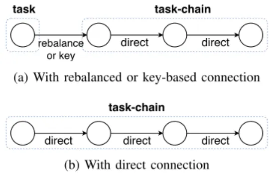
Fig. 5: Flink task sub-chaining with different connections In most platforms, like Storm, every task is managed as a single entity and placed independently from the others. Moreover, the connection between tasks has to be specified. Meanwhile, Flink introduces a task-chaining concept. With default routing, Flink directly connects tasks with the same parallelism level (Fig. 5). They form a direct chain of sub-tasks that can communicate directly, bypassing the network layer. These chains are treated as a single entity and scheduled as such. In the current version of NAMB, whereas in Storm and Heron the specified routing is applied between each task, in Flink it is only applied at the first level, between the source and the first-level tasks. This preserves the chains of sub-tasks and produces a more realistic and optimized prototype.

While the majority of applications generators perform also query optimization, it is not our main focus. Our objective is to generate prototypes. For this reason, we take into account platform specifics only to make design decisions for the gen-eration. However, it would be easy for someone to implement an optimized generator for a specific platform, taking into account the previously described design rules and the internal mechanisms of the platform.

C. Task Workload Simulation

To maintain the general nature of NAMB, the user does not have to specify the exact code of a task. This avoids specific query operations on data, resulting in context-specific scenarios. Instead, NAMB simulates the load through a busy-wait loop function (see Fig. 2). In this manner it is able to simulate processing workload, easily configurable in the schema. A parameter is used to set the number of loop cycles, allowing NAMB to replicate the processing load of common tasks used in stream processing.

To demonstrate the equivalence that can be obtained be-tween busy-wait loops and a real load, we have performed experiments on Apache Storm (version 1.2.1) on a 4-core node. Based on a set of representative works in the DSP domain [12], [17], [16], [28], [29] we derived 5 key DSP tasks:

1) Identity: a task that just forwards the tuple as it is, without any processing;

2) Transformation: a task that transforms the input data, e.g. a parsing function that divides a JSON or XML text into an array of fields;

3) Filter: a task that filters data based on its value or a specific field, e.g. if/else rules;

4) Aggregation: a task that accumulates the input data over time, e.g. arithmetic operations;

5) Sorting: a task that sorts in a specific order the input data over time, e.g. ranking of word occurrences.

iden. filter aggr. rank. transf. 0 100 200 300 400 500 600 CPU Time (ms)

(a) Common tasks

0.7 103 450

BusyWait Cycles (Thousands of) 0 100 200 300 400 500 600 CPU Time (ms) (b) Simulated tasks Fig. 6: Per tuple CPU measurements for real/simulated tasks

Each of these tasks was executed and its CPU time measured using Java’s ThreadMXBean[30] API (Fig. 6a). Then busy-wait (i.e. simulated load) tasks were created and evaluated in the same conditions. With a carefully chosen number of cycles, we were able to reproduce a load similar to the original task. For example, Fig. 6b shows that the aggregation (resp. transformation) task can be approximated with a busy-wait of 700 (resp. 450,000) cycles.

VIII. EVALUATION

In this section, we present different scenarios where we use NAMB to make quick and easy evaluations of SPEs using prototype applications.

All the experiments were done on a 4-node Linux cluster on the Grid’5000 testbed. Each node has two 4-core Intel Xeon CPUs and 32GB of memory interconnected by a 1 Gbps network. One machine is used as master and the other 3 as worker nodes. The presented experiments have been done on Flink and Storm.

We use throughput and processing latency as the two evaluation metrics. The throughput is measured as the total number of tuples produced by the sources per millisecond. The processing latency is the average time spent by tuples between the source and the sink. We set the output sample to be 1 every 2000 tuples, to give us enough data to obtain representative statistics, while still not overloading the system with continuous logging.

A. Application Design

To demonstrate the benefits of the Workflow schema, we show how starting from a common linear topology, we can quickly evaluate the impact of small changes in the design

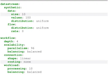
choices. We evaluate it on Flink with 2 different micro-benchmarks, using the base configuration file shown in Fig. 7. For each experiment, we focus on a single parameter change (highlighted in gray in the figure). The considered topology is made of single source and 3 tasks organized in a linear layout with a balanced parallelism distribution. The topology is fed with a uniform synthetic data stream of 100 unique values of 10 bytes each, without rate limit.

datastream: synthetic: data: size: 10 values: 100 distribution: uniform flow: distribution: uniform rate: 0 workflow: depth: 4 scalability: parallelism: 96 balancing: balanced connection: shape: linear routing: none workload: processing: 10 balancing: balanced

Fig. 7: Base configuration file for Workflow schema experi-ments. Highlighted values are changed during tests

1) Connection Routing: In this test, we analyze the impact on the performance of the different routing systems of Flink. We fix the parallelism level to 96, the upper-bound imposed by Flink in our hardware environment [31].

We test three different grouping schemes by changing the routing type parameter. The direct connection (none value in the configuration) directly connects the source to the task. As a consequence, Flink groups all the tasks in the same chain, as explained above. The rebalance routing (balanced in NAMB) equally distributes the tuples between all task instances. And finally, grouping by key (hash), distributes the tuples based on the hash value of the tuple. For these last two methods, Flink creates two different tasks (Fig. 5a), therefore the tuples will need to travel the network to be routed to the assigned task (i.e, the network layer is not bypassed with the sub-chain approach).

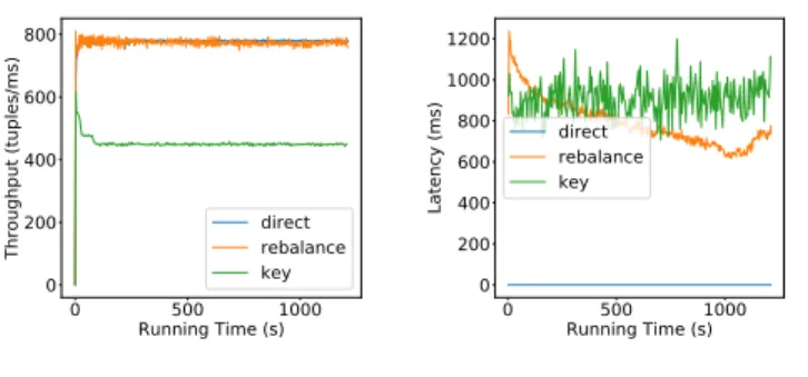
In Fig. 8b we can immediately see a significant impact on latency when the tasks are directly connected and co-placed: the latency is significantly lower than the other two methods, only 0.03 ms of average completion time compared to the 701 ms and the 907 ms for balanced and hash respectively. Both balancing and direct routing achieve the same throughput (Fig. 8a) while the key-based (i.e. hashed) grouping offers significantly lower performance.

2) Data Size: Another important factor to take into account when developing an application is the size of data. In most cases, the data will have to be transferred between machines, impacting the overall performance of the application.

0 _{Running Time (s)}500 1000 0 200 400 600 800

Throughput (tuples/ms) directrebalance key

(a) Throughput; higher is better

0 _{Running Time (s)}500 1000 0 200 400 600 800 1000 1200 Latency (ms) direct rebalance key

(b) Latency; lower is better Fig. 8: Performance with different connection routing between source and task.

This test explores three different data sizes, 2, 10, and 100 Bytes, representing a number, a string and a JSON message respectively. We will use a balanced routing strategy to ensure to have network communication but without the overhead of the hash functions.

Fig. 9a shows that the data size has a modest influence on the throughput. However, the impact on the latency is high. The larger the tuples, the lower the latency (Fig. 9b). Flink uses internal buffers [32] which are flushed either after some timeout expires or when they are full. Having large tuples triggers the second condition faster, decreasing the overall latency. 0 500 1000 Running Time (s) 0 200 400 600 800

Throughput (tuples/ms) 2 bytes10 bytes

100 bytes

(a) Throughput; higher is better

0 500 1000 Running Time (s) 400 600 800 1000 1200 Latency (ms) 2 bytes 10 bytes 100 bytes

(b) Latency; lower is better Fig. 9: Performances with different data sizes, balanced routing

In this section, we have shown how NAMB can be used to quickly generate a set of prototypes. By slightly modifying the configuration file, a user can investigate the impact of multiple different features of a DSP.

B. Platform Mechanisms

We use here the Workflow schema to quickly test specific platform mechanisms. In this experiment, we analyze the back-pressure mechanism of Storm, enabled by the acking frame-work [25]. Back-pressure ensures a limit to the application throughput, to avoid overloading the system in case of a too high rate of incoming tuples. The acking framework is also used to ensure message reliability. Its activation in Storm requires adding specific code in every task. In NAMB, this can be done by simply setting the reliability parameter to true in the workload section.

Our purpose is to stress the system to trigger the back-pressure mechanism. We use multiple Kafka producers and a Kafka server to generate an high rate of tuples. The latter (Fig. 10) is co-located in the master server.

The generated prototype is a source with two tasks in a linear topology, with a processing of 0 for each task, so as to let the application reach the maximum throughput.

datastream: external: kafka: server: <master_server>:9092 group: test topic: test zookeeper: server: <master_server>:2181 workflow: depth: 3 scalability: parallelism: 3 balancing: balanced connection: shape: linear routing: balanced workload: processing: 0 reliability: true

Fig. 10: Configuration file for the back-pressure experiment. The external Kafka producer is set to have two production phases. Most of the time it is in a steady phase, with a fixed data generation rate. However, at regular intervals, the rate is increased during a so-called burst phase. We tested Storm once with the reliability mechanism enabled and once with it disabled. 0 200 400 600 800 Running Time (s) 0 20 40 60 80 100 Throughput (tuples/ms) storm kafka (a) Enabled 0 200 400 600 800 Running Time (s) 0 20 40 60 80 100 Throughput (tuples/ms) storm kafka (b) Disabled

Fig. 11: Back-Pressure test in Storm, with enabled and dis-abled reliability mechanism.

In Fig. 11a, with reliability enabled, the back-pressure limits the throughput to 80 tuples/ms during burst phases, which is lower than the Kafka production rate (over 100 tuples/ms). After completing the processing of all the Kafka tuples, Storm throughput goes back to the steady phase. On the contrary, we can see in Fig. 11b, how, without the reliability mechanism enabled, the application almost immediately fails. Even during the steady phase, it cannot process incoming tuples fast enough, leading to out-of-memory errors.

C. Real Application Prototyping

Using the Pipeline schema, we can reproduce existing applications and create prototypes with similar performance.

For this evaluation, we use the Yahoo! Streaming Benchmark (see Fig. 1 and Section II-A). To validate our approach, we compare the results on two different platforms: Storm and Flink. As in [10], we have modified the Yahoo Streaming Benchmark to remove the Kafka producer and use a local ad-hoc data generator instead, so as to maximize the application throughput. Throughput Latency 10.0 7.5 5.0 2.5 0.0 2.5 5.0 7.5 10.0

NAMB / YahooBench difference (%)

(a) Apache Storm

Throughput Latency 10.0 7.5 5.0 2.5 0.0 2.5 5.0 7.5 10.0

NAMB / YahooBench difference (%)

(b) Apache Flink Fig. 12: Throughput and latency percentage difference ratio between NAMB and Yahoo Bench results

Fig. 12 shows the relative difference between NAMB and the Yahoo Streaming application for both platforms. We can see that NAMB is able to obtain almost the same performance as the original application. The Yahoo Benchmark in Storm (Fig. 12a) reaches a throughput of 102 tuples/ms, whereas NAMB achieves 107 tuples/ms, less than 5% difference. Meanwhile, the average latency is around 48 ms with the YahooBench and 50 ms with NAMB (slightly more than a 3% difference). The difference with Flink is similar in terms of throughput with only a 1.5% difference, 129 tuples/ms for the YahooBench vs 127 tuples/ms with NAMB). The difference in latency is 4%,15 ms with the YahooBench and 14.5 ms with NAMB.

From these results, we can observe that Flink gives slightly better performance. This is because of its task grouping policy, which reduces network communications. Storm, on the other hand, uses 6 Java Virtual Machines.

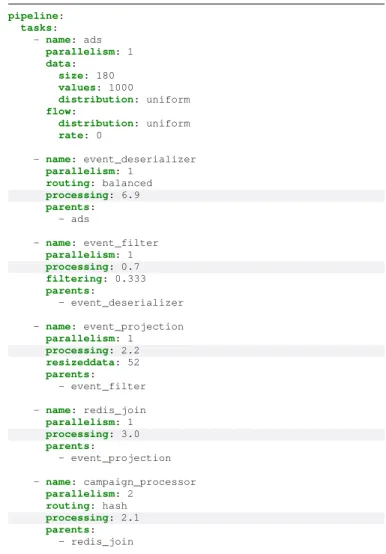
In Fig. 13 we see, as an example, the configuration used for Storm. For these two experiments, we did not use the same configuration file. Indeed, the computational load of Storm and Flink is different for the same application (Section VII-B). We adapted the processing loads in Flink to be 60% of the ones used in Storm. This was, however, the only difference. The rest of the configuration parameters being strictly identical. D. Bottleneck Discovery

Once found the correct configuration for the Yahoo! Bench-mark, we can exploit NAMB’s flexibility to investigate the be-havior of an application under various conditions. We consider a scenario where developers are interested in finding potential bottlenecks in their application. Without lose of generality, we chose Flink as SPE.

We used the base configuration shown in Fig. 13 (exper-iment base). We used two others configurations as possible

pipeline: tasks: - name: ads parallelism: 1 data: size: 180 values: 1000 distribution: uniform flow: distribution: uniform rate: 0 - name: event_deserializer parallelism: 1 routing: balanced processing: 6.9 parents: - ads - name: event_filter parallelism: 1 processing: 0.7 filtering: 0.333 parents: - event_deserializer - name: event_projection parallelism: 1 processing: 2.2 resizeddata: 52 parents: - event_filter - name: redis_join parallelism: 1 processing: 3.0 parents: - event_projection - name: campaign_processor parallelism: 2 routing: hash processing: 2.1 parents: - redis_join

Fig. 13: Pipeline schema configuration file used for Storm. Highlighted values differ in the Flink configuration.

optimizations: one where we halved the processing load of the event deserializer(experiment A); and another where we made the same optimization to the campaign processor (experiment B). The goal is to evaluate the impact of some potential code optimization on these two components.

base A B 0 50 100 150 Throughput (tuples/ms)

(a) Throughput: higher is better

base A B 0 5 10 15 Latency (ms)

(b) Latency: lower is better Fig. 14: Bottleneck discovery experiment in the three different configurations

The results of the evaluation in Fig. 14a shows that, in terms of throughput, the event deserializer is one of the possible

bottlenecks in the application. Meanwhile, reducing the load of the campaign processor does not have an impact on through-put. On the other hand, considering the latency (Fig. 14b), we see that in both cases we have an improvement of the tuples processing time. Yet, halving the event deserializer produces a more substantial improvement.

IX. CONCLUSION

In this paper, we have presented NAMB, Not only A Micro-Benchmark, a generic application prototype generator. Based on the analysis of the main characteristics of DSP applica-tions, we have devised two high-level description models for streaming topologies. They allow for the precise, high-level, definition of an application workflow. The first one, the Work-flow schema, can be used to quickly write prototypes for a set of canonical topologies. The second one, the Pipeline schema, can accurately reproduce complex applications. NAMB uses these models to produce a working streaming application prototype for a target platform.

To remain platform- and application-independent, we simu-late the tasks processing workload, through an equivalent busy-wait function. A Data Generation component, with support for synthetic and external data, is used to inject tuples to the application.

Through numerous experiments, we have shown how NAMB can be used to quickly define and run prototyped applications over multiple platforms. We used Flink to show the impact of small design choices, such as data routing and size. Through Storm we showed how one can quickly study the behavior of internal platform mechanisms, along with tasks performance optimization evaluation. We finally used both systems to show how NAMB could replicate more com-plex and realistic applications, through the Yahoo Streaming Benchmark, achieving the same performance as the original one.

The current version of NAMB, along with the configuration files used in this paper, is available on GitHub. It supports Storm, Flink and Heron. The implementation of Spark Stream-ing is currently undergoStream-ing, along with an extension to the Synthetic Generator to support more complex distribution functions.

ACKNOWLEDGMENTS

Experiments presented in this paper were carried out using the Grid’5000 testbed, supported by a scientific interest group hosted by Inria and including CNRS, RENATER and several Universities as well as other organizations (see https://www. grid5000.fr).

REFERENCES [1] “Apache Flink,” http://flink.apache.org/. [2] “Apache Storm,” http://storm.apache.org/.

[3] “Apache Heron,” https://apache.github.io/incubator-heron/. [4] “Apache Spark Streaming,” https://spark.apache.org/streaming/. [5] T. Akidau, A. Balikov, K. Bekiro˘glu, S. Chernyak, J. Haberman, R. Lax,

S. McVeety, D. Mills, P. Nordstrom, and S. Whittle, “Millwheel: fault-tolerant stream processing at internet scale,” PVLDB, 2013.

[6] A. Pagliari, F. Huet, and G. Urvoy-Keller, “Towards a high-level descriotion for generating stream processing benchmark applications,” in IEEE BigData, 2019.

[7] A. Arasu, M. Cherniack, E. Galvez, D. Maier, A. S. Maskey, E. Ryvkina, M. Stonebraker, and R. Tibbetts, “Linear road: a stream data manage-ment benchmark,” in PVLDB, 2004.

[8] S. Chintapalli, D. Dagit, B. Evans, R. Farivar, T. Graves, M. Holder-baugh, Z. Liu, K. Nusbaum, K. Patil, B. J. Peng et al., “Benchmarking streaming computation engines: Storm, flink and spark streaming,” in IEEE IPDPSW, 2016.

[9] J. Grier, “Extending the Yahoo! Streaming Benchmark,” https://www. ververica.com/blog/extending-the-yahoo-streaming-benchmark, 2016. [10] B. Yavuz, “Benchmarking Structured Streaming on Databricks

Runtime Against State-of-the-Art Streaming Systems,” https: //databricks.com/blog/2017/10/11/benchmarking-structured-streaming-on-databricks-runtime-against-state-of-the-art-streaming-systems.html, 2017.

[11] A. Krettek, “The Curious Case of the Broken Benchmark: Revisiting Apache Flink® vs. Databricks Runtime,” https: //www.ververica.com/blog/curious-case-broken-benchmark-revisiting-apache-flink-vs-databricks-runtime, 2017.

[12] B. Peng, M. Hosseini, Z. Hong, R. Farivar, and R. Campbell, “R-storm: Resource-aware scheduling in storm,” in ACM Middleware, 2015. [13] R. Lu, G. Wu, B. Xie, and J. Hu, “Stream bench: Towards benchmarking

modern distributed stream computing frameworks,” in IEEE/ACM UCC, 2014.

[14] L. Wang, J. Zhan, C. Luo, Y. Zhu, Q. Yang, Y. He, W. Gao, Z. Jia, Y. Shi, S. Zhang et al., “Bigdatabench: A big data benchmark suite from internet services,” in IEEE HPCA, 2014.

[15] “Alibaba Jstorm,” https://github.com/alibaba/jstorm.

[16] A. Shukla, S. Chaturvedi, and Y. Simmhan, “Riotbench: An iot bench-mark for distributed stream processing systems,” Wiley Concurrency, 2017.

[17] S. Chatterjee and C. Morin, “Experimental study on the performance and resource utilization of data streaming frameworks,” in IEEE/ACM CCGRID, 2018.

[18] M. Hirzel, G. Baudart, A. Bonifati, E. Della Valle, S. Sakr, and A. Akrivi Vlachou, “Stream processing languages in the big data era,” ACM SIGMOD, 2018.

[19] T. Akidau, R. Bradshaw, C. Chambers, S. Chernyak, R. J. Fern´andez-Moctezuma, R. Lax, S. McVeety, D. Mills, F. Perry, E. Schmidt et al., “The dataflow model: a practical approach to balancing correctness, latency, and cost in massive-scale, unbounded, out-of-order data pro-cessing,” PVLDB, 2015.

[20] “Apache Beam,” https://beam.apache.org/.

[21] I. Botan, R. Derakhshan, N. Dindar, L. Haas, R. J. Miller, and N. Tatbul, “Secret: a model for analysis of the execution semantics of stream processing systems,” PVLDB, 2010.

[22] G. Mencagli, P. Dazzi, and N. Tonci, “Spinstreams: a static optimization tool for data stream processing applications,” in AMC Middleware, 2018. [23] P. G¨otze, W. Hoffmann, and K.-U. Sattler, “Rewriting and code

gener-ation for dataflow programs.” in GvD, 2016.

[24] C. Olston, B. Reed, U. Srivastava, R. Kumar, and A. Tomkins, “Pig latin: a not-so-foreign language for data processing,” in ACM SIGMOD, 2008.

[25] A. Pagliari, F. Huet, and G. Urvoy-Keller, “On the cost of reliability in data stream processing systems,” in IEEE/ACM CCGRID, 2019. [26] “YAML,” https://yaml.org/.

[27] J. Karimov, T. Rabl, A. Katsifodimos, R. Samarev, H. Heiskanen, and V. Markl, “Benchmarking distributed stream data processing systems,” in IEEE 34th ICDE, 2018.

[28] G. Hesse, B. Reissaus, C. Matthies, M. Lorenz, M. Kraus, and M. Uflacker, “Senska–towards an enterprise streaming benchmark,” in Springer TPCTC, 2017.

[29] M. ˇCerm´ak, D. Tovarˇn´ak, M. Laˇstoviˇcka, and P. ˇCeleda, “A performance benchmark for netflow data analysis on distributed stream processing systems,” in IEEE/IFIP NOMS, 2016.

[30] “Java Thread MX Bean,” https://docs.oracle.com/javase/8/docs/api/java/ lang/management/ThreadMXBean.html.

[31] “Apache Flink Job Scheduling,” https://ci.apache.org/projects/flink/flink-docs-release-1.7/internals/job scheduling.html.

[32] N. Kruber, “A Deep-Dive into Flink’s Network Stack,” https://flink. apache.org/2019/06/05/flink-network-stack.html.