HAL Id: hal-01083199
https://hal.archives-ouvertes.fr/hal-01083199
Submitted on 16 Nov 2014HAL is a multi-disciplinary open access
archive for the deposit and dissemination of sci-entific research documents, whether they are pub-lished or not. The documents may come from teaching and research institutions in France or abroad, or from public or private research centers.
L’archive ouverte pluridisciplinaire HAL, est destinée au dépôt et à la diffusion de documents scientifiques de niveau recherche, publiés ou non, émanant des établissements d’enseignement et de recherche français ou étrangers, des laboratoires publics ou privés.
estimations to observed hydrometeorological variability
Pierre Brigode, Pietro Bernardara, Emmanuel Paquet, Joël Gailhard, Federico
Garavaglia, Ralf Merz, Zoran Mićović, Deborah Lawrence, Pierre Ribstein
To cite this version:
Pierre Brigode, Pietro Bernardara, Emmanuel Paquet, Joël Gailhard, Federico Garavaglia, et al.. Sensitivity analysis of SCHADEX extreme flood estimations to observed hydrometeorolog-ical variability. Water Resources Research, American Geophysical Union, 2013, 50, pp.1-18. �10.1002/2013WR013687�. �hal-01083199�
Page 1 on 28
Sensitivity analysis of SCHADEX extreme flood estimations to
observed hydrometeorological variability
Pierre Brigode,1,2 Pietro Bernardara,1 Emmanuel Paquet,3 Joël Gailhard,3 Federico Garavaglia,3 Ralf Merz,4 Zoran
Mićović,5 Deborah Lawrence,6 and Pierre Ribstein2
Received 15 February 2013; revised 2 December 2013; accepted 4 December 2013.
Abstract: Stochastic flood simulation methods are typically based on a rainfall probabilistic model (used for simulating continuous rainfall series or for estimating probabilities of random rainfall events) and on a rainfall-runoff model. Usually, both of these models are calibrated over observed hydrometeorological series, which may be subject to significant variability and/or nonstationarity over time. The general aim of this study is thus to propose and test a methodology for performing a sensitivity analysis of extreme flood estimations to observed hydrometeorological variability. The methodology consists of performing a set of blockbootstrap experiments: for each experiment, the data used for calibration of a particular model (e.g., the rainfall probabilistic model) is bootstrapped while the model structure and the calibration process are held constant. The SCHADEX extreme flood estimation method has been applied over six catchments located in different regions of the world. The results show first that the variability of observed rainfall hazard has the most significant impact on the extreme flood estimates. Then, consideration of different rainfall-runoff calibration periods generates a significant spread of extreme flood estimated values. Finally, the variability of the catchment saturation hazard has a nonsignificant impact on the extreme flood estimates. An important point raised by this study is the dominating role played by outliers within the observed records for extreme flood estimation.
Citation: Brigode, P., P. Bernardara, E. Paquet, J. Gailhard, F. Garavaglia, R. Merz, Z. Mic´ovic´, D. Lawrence, and P. Ribstein (2013), Sensitivity analysis of SCHADEX extreme flood estimations to observed hydrometeorological variability, Water Resour. Res., 49, doi:10.1002/2013WR013687.
1 LNHE, R&D, Electricité de France, Chatou, France.
2 UMR 7619 Sisyphe, Université Pierre et Marie Curie, Paris, France. 3 DTG, DMM, Electricité de France, Grenoble, France.
4 Department of Catchment Hydrology, UFZ Helmholtz Centre for Environmental Research, Halle, Germany. 5 BC Hydro, Engineering, Burnaby, British Columbia, Canada.
6 Norwegian Water Resources and Energy Directorate (NVE), Oslo, Norway.
Corresponding author: P. Brigode, LNHE, R&D, Electricité de France, 6 quai Watier, FR-78401 Chatou CEDEX, France. ([email protected])
Page 2 on 28
1 INTRODUCTION
1.1 Uncertainty of Extreme Flood Estimations
Extreme flood estimation methods have been developed over many years and represent the combined work of the hydrological and statistical communities. These methods allow one to define a probability distribution for extreme streamflows and thus to assign an average return period to extreme streamflow values based on their probability. Validation of proposed extreme flood estimates is critical but not easily achieved, as extreme flood observations are by definition very rare. In some cases, historical events which occurred prior to an observed streamflow series can be used to represent events over longer timescales [e.g., Payrastre et al., 2011], although there is much uncertainty associated with such extrapolations. Moreover, the observed hydrometeorological series used for the calibration of an extreme flood estimation method may be subject to significant variability over time [Milly et al., 2002], e.g., due to changes in the catchment or river engineering works or even, due to global climate oscillations such as the El Niño Southern Oscillation. Given that the assessment of the full range of uncertainty underlying a flood estimate is a difficult task [Merz and Thieken, 2005], investigating to what extent the proposed extreme flood values are dependent on the data used for calibration of the method is an important first step. How to quantify this sensitivity depends on the flood estimation method considered (e.g., flood frequency analysis, stochastic simulation methods).
1.2 Classical Flood Frequency Analysis
Usually, the probability distribution of the extreme floods is defined by fitting a given probability distribution to the sample of streamflow observations available at the considered site [Singh and Strupczewski, 2002], using extreme value theory [Fréchet, 1927; Gumbel, 1958]. Flood frequency analysis is based on hypotheses of independent and identically distributed properties with respect to the streamflow series considered. Whether or not these hypotheses are met has been questioned [see e.g., Klemeš, 2000a, 2000b] and inconsistencies have been found in different world regions such as New South Wales (Australia) where climate oscillations influence significantly the annual maximum streamflow series [Franks and Kuczera, 2002; Micevski et al., 2006] and the Mekong Basin (Southeast Asia) where the interannual variability of the Western North Pacific monsoon significantly influences lower Mekong river flood regimes [Delgado et al., 2010]. Moreover, the choice of the probability distribution for flood frequency analysis is usually based on the statistical properties and on the fit of the data to the probability distribution instead of on a physical consideration of the underlying phenomena leading to, for example, a decomposition of the different processes involved in generating floods [Merz and Blöschl, 2008a, 2008b]. Due to this absence of decomposition, classical flood frequency analysis are no adapted to such sensitivity analysis.
1.3 Stochastic Simulation Methods
Approaches based on the statistical analysis of flood streamflow samples simulated by rainfall-runoff models which are forced by simulated rainfall have appeared in the scientific literature over the past two decades [see e.g., Calver and Lamb, 1995; Franchini et al., 1996; Cameron et al., 1999; Blazkova and Beven, 2002; Sivapalan et al., 2005; Hingray and Mezghani, 2008]. These approaches are referred to as ‘‘stochastic simulation methods’’ [see Boughton and Droop, 2003 for a review], and they are typically composed of a probabilistic rainfall model coupled with a rainfall-runoff model. The main advantage of these approaches is that the large flood streamflow samples simulated by the rainfall-runoff models should, in principle, reproduce the relevant flood-generating physical mechanisms and that the dynamics of the hydroclimatological processes driving flood generation are also implicitly represented [Lamb, 1999]. Moreover, these methods propose a decomposition of the flood-producing factors, which is particularly interesting in a sensitivity analysis framework.
Stochastic simulation methods can be developed within a continuous simulation framework or as a single or series of event-based simulations. The first of these methods necessitates the use of a continuous stochastic rainfall model in order to generate a continuous input for the rainfall-runoff model for the simulation of a continuous streamflow series. Continuous stochastic simulation approaches are thus based on a two-part decomposition of the flood-producing factors: (i) the rainfall hazard described by a stochastic rainfall model and (ii) the hydrological hazard described by a rainfall-runoff model. Due to this decomposition into driving factors and hydrological response factors, a sensitivity analysis is potentially more informative for continuous stochastic
Page 3 on 28
simulation methods than for classical statistically based flood frequency approaches. Several studies have shown that continuous stochastic rainfall models are able to reproduce a range of observed rainfall characteristics [e.g., Rodriguez-Iturbe et al., 1987; Cowpertwait, 1995; Schmitt et al., 1998; Arnaud and Lavabre, 1999; Willems, 1999; Olsson and Burlando, 2002; Bernardara et al., 2007; Papalexiou et al., 2011]. However, reproducing both the distribution of wet and dry rainfall periods and the magnitude of heavy rainfall events is a challenging task [e.g., Lennartsson et al., 2008]. Thus, Rogger et al. [2012] recently highlighted the complexity of stochastic rainfall models as a limitation of continuous simulation methods. The complexity of the extreme streamflow estimation exercise is not only due to the stochastic rainfall model but also to the rainfall-runoff model used to describe the catchment saturation hazard [e.g., Verhoest et al., 2010; Li et al., 2012; Pathiraja et al., 2012]. Moreover, Sivapalan et al. [2005] showed that it is necessary to take into account the seasonality of flood generating processes, especially when the rainfall hazard and the catchment saturation hazard are not in phase.
Several complete sensitivity analysis approaches have also been proposed for continuous simulation methods. The sensitivity of extreme flood estimations to the catchment saturation hazard has been highlighted by Franchini et al. [1996] by performing continuous simulations with different values of the rainfall-runoff model parameters controlling catchment saturation hazard. Cameron et al. [1999] and Blazkova and Beven [2002] quantified extreme flood estimation uncertainties using the GLUE methodology [Beven and Binley, 1992] for both the calibration of the rainfall-runoff model and for the calibration of the stochastic rainfall generator. Lamb [1999] tested four different objective functions for the calibration of a rainfall-runoff model used within a continuous simulation process and showed that objective function used for calibration of the rainfall-runoff model influenced significantly the extreme flood estimation. Finally, Hashemi et al. [2000] and Franchini et al. [2000] highlighted the existing interactions between the different parameters of a continuous simulation method and their impacts on extreme flood estimations.
Stochastic event-based simulation methods do not require continuous stochastic rainfall model, but only the simulation of a single or set of rainfall events. Rainfall-runoff models are thus fed with simulated rainfall events to produce flood events. These approaches must adequately reproduce a three-part decomposition of flood-producing factors: (i) the rainfall hazard described with stochastic rainfall models, (ii) the catchment saturation hazard described with hydroclimatological records, and (iii) the rainfall-runoff transformation described with rainfall-runoff models. Stochastic event-based simulation methods are, due to their relative simplicity and fast computational times, widely applied in engineering hydrology, such as the design storm procedure. In this procedure, a particular storm with a known return period is used as an input to an event rainfall-runoff model [e.g., Pilgrim and Cordery, 1993, pp. 9–13]. It is then assumed that the simulated peak discharge has the same return period as the storm [e.g., Bradley and Potter, 1992]. However, this pragmatic assumption clearly does not account for the role of different processes in determining the relationship between the frequencies of the design rainfall and the derived flood peak, and the resulting return period of the runoff is often overestimated. The relationship between event rainfall and flood runoff probability, often termed as mapping of rainfall to flood return period, is subject of an ongoing scientific discussion [see e.g., Viglione and Blöschl, 2009; Viglione et al., 2009].
1.4 Scope of the Paper
Using the three-part decomposition of the flood-producing factors inferred by event-based stochastic flood simulation approach, the general aim of this study is to quantify the sensitivity of extreme flood estimations obtained through such methods to the data used for calibration. The sensitivity analysis methodology is thus based on this three-part decomposition and aims at quantifying and comparing the sensitivity of extreme flood estimations to (i) the rainfall hazard, to (ii) the catchment saturation hazard, and to (iii) the rainfall-runoff transformation. These three factors are first independently investigated, and a general sensitivity analysis combining the three flood-producing factors is then performed in order to highlight which of these three factors is most sensitive to difference in calibration data. The methodology is based on the nonparametric bootstrap concept, initially proposed by Efron [1979], and consists of performing a set of block-bootstrap experiments. For each bootstrap experiment performed, the data used for calibration of a particular model (e.g., the rainfall probabilistic model) is bootstrapped while the model structure and the calibration process are held constant, in order to quantify the sensitivity of the extreme flood estimation method to the particular factor considered. Note that similar methodologies have been already used for quantifying the dependence of rainfall-runoff model parameters to the calibration period considered [e.g., Gan and Burges, 1990; Choi and Beven, 2007; Le Lay et al., 2007; Vaze et al., 2010; Seiller et al., 2012; Coron et al., 2012; Brigode et al., 2013a].
Page 4 on 28
The methodology will be tested using several applications of the SCHADEX (Simulation Climato-Hydrologique pour l’Appréciation des Débits EXtrêmes) method. SCHADEX is a ‘‘semicontinuous’’ stochastic simulation method proposed by Paquet et al. [2006, 2013], Garavaglia [2011] in which the rainfall hazard is simulated on an event-basis while the catchment saturation hazard is simulated through continuous rainfall-runoff modeling. The method is currently in operational use and has been used at Electricité De France (EDF) since 2006 for estimating design floods for dam spillway design. The sensitivity analysis of the SCHADEX method will be illustrated using six catchments located in different regions of the world and which are characterized by considerable differences in flood seasonality and flood generation mechanisms. The SCHADEX methodology and the bootstrap methodology used is described in section 2, the data sets used are presented in section 3, results obtained are summarized and discussed in section 4, and section 5 presents conclusions.
2 METHODOLOGY
2.1 The SCHADEX Method: A Monte-Carlo Simulation for Extreme Floods
Estimation
2.1.1 SCHADEX Overview
A brief description of the SCHADEX method and principles is given in this subsection (for a complete presentation, see Paquet et al. [2013]).
Within the SCHADEX method, extreme floods are assumed to result from the combination of two natural hazards: the precipitation hazard and the catchment saturation hazard. The general idea behind SCHADEX is thus to exhaustively mix these two hazards within a stochastic simulation framework based on a rainfall-runoff model. Note that the SCHADEX stochastic simulation framework applied here uses a daily time-step, although subdaily applications are also possible. A lumped, conceptual rainfall-runoff model is used here (described in subsection 2.1.3), meaning that input series should represent areal averaged values for the catchment.
The SCHADEX stochastic simulation framework is a semicontinuous simulation process. Indeed, the areal rainfall hazard is simulated on an event basis, while the catchment saturation hazard is simulated through continuous rainfall-runoff modeling. Rainfall events are simulated rather than a continuous rainfall series. This allows avoiding the complex probabilistic modeling of the structure and intermittency of dry and wet subperiods. The event duration is a priori fixed to 3 days, and the rainfall events are supposed to have a ‘‘triangular shape’’ (i.e., with a central daily rainfall amount greater than the one in the previous and the following days). The probability distribution of the central (and thus maximum) rainfall considered in this study is described in section 2.1.2. Catchment saturation conditions are not stochastically generated but they are rather sampled from the catchment saturation conditions simulated by the rainfall-runoff model forced by historical series of meteorological input (areal rainfall and temperature series), described in the subsection 2.1.4. Rainfall and catchment saturation hazards are then coupled, by injecting simulated synthetic rainfall events into the rainfall-runoff simulation. In order to respect the empirical correlation between catchment saturation conditions and rainfall event occurrence, the simulated rainfall events are introduced into the historical rainfall-runoff simulation only where central rainfall events (observed rainy days greater than the previous and the following days) were actually observed, thus replacing the observed events. Thus, the time steps for the synthetic rainfall event injection are the time steps of the historical record where central rainfall events are observed. Finally, up to 23106 different synthetic rainfall events are injected for a complete SCHADEX simulation; several hundred events are thus generated and injected independently for each observed central day.
SCHADEX final results are thus constituted of millions of simulated floods resulting from different combinations of extreme rainfall events and catchment saturations for each catchment considered. These results are summarized by a Cumulative Distribution Function (CDF) describing daily streamflows simulated by SCHADEX as a function of their empirical return-periods. Note that this representation of the SCHADEX results is a summary of the entire variety of simulated floods, since seasonal or monthly distributions of SCHADEX simulated floods could be plotted and analyzed. Seasonal patterns of the combination of extreme rainfall hazard and catchment saturation hazard are indeed particularly interesting to quantify in order to understand main flood-producing process involved over the studied catchment [Sivapalan et al., 2005].
Page 5 on 28
2.1.2 Probabilistic Rainfall Model
The Multi-Exponential Weather Pattern (MEWP) probabilistic model [Garavaglia et al., 2010, 2011] has been used in this study. It is based on a seasonal and weather pattern (WP) subsampling of precipitation series. A WP classification has thus to be defined at the regional scale prior to the definition of the MEWP model. An exponential law is used to model each of the considered subsamples (one subsample for each season and each WP). Finally, a global MEWP distribution is defined for each catchment as the combination of all the different exponential laws. The combination is weighted by the frequency of each WP central rainfall observations. The formulation of the MEWP distribution for one particular season is given in equation (1), where i is the studied season, CR are the Central Rainfall observations, j is the studied WP, nWP is the number of WP, p is the CR event
probability of occurrence of the WP, F is the marginal distribution, u is the threshold for heavy rainfall observation selection, and k is the parameter of the exponential law. Note that we have used here CR to indicate rainfall in order to highlight that the MEWP distributions are not defined, in the SCHADEX framework, using the entire observed precipitation series, but rather, using the central rainfall sample, thus providing a type of Peak-Over-Threshold (POT) sampling of observed daily rainfall series.
𝐹𝑖(𝐶𝑅) = ∑ 𝐹 𝑗𝑖 𝑛𝑊𝑃 𝑗=1 (𝐶𝑅) ∗ 𝑝𝑗𝑖 (1) 𝐹𝑖(𝐶𝑅) = ∑ [1 − 𝑒𝑥𝑝 (−𝐶𝑅 − 𝑢𝑗 𝑖 𝜆𝑗𝑖 )] 𝑛𝑊𝑃 𝑗=1 ∗ 𝑝𝑗𝑖
The relation between MEWP probability and return period is given in the equation (2), where T is the return period in years, n is the size of the rainfall observation subsample considered, N is the number of years of the CR series considered.
𝑇(𝐶𝑅) = 1
1 − 𝐹(𝐶𝑅)𝑁𝑛 (2)
As stated in section 1, the use of WP classifications for rainfall subsampling represents the main novelty of the MEWP probabilistic model. Moreover, this probabilistic model has been compared with other standard probabilistic models and highlighted as a robust and reliable model over daily rainfall data of France, Spain, and Switzerland [Garavaglia et al., 2011].
2.1.3 Rainfall-Runoff Model
Within the SCHADEX method, a rainfall-runoff model is needed for two goals: (i) to model the catchment saturation hazard on the considered catchment and (ii) to transform several thousand ‘‘extreme synthetic rainfall event’’ inputs into extreme floods. The rainfall-runoff model has to, therefore, be calibrated for both objectives, i.e., good performances for the average hydrological behavior of the considered catchment (hydrological regime) and the heavy floods observed on the considered catchment.
One daily continuous lumped rainfall-runoff model has been used in this study: the MORDOR model [Garçon, 1999], developed at EDF and applied over the past 15 years in many contexts, such as operational flow forecasting (from several hours to several days in advance), seasonal inflows forecasting, hydrological studies, climate change analysis, and others. The MORDOR version used here has a snowpack component, which is used for catchments where snow processes are not negligible. The MORDOR version without the snowpack component has 11 free parameters, while the full MORDOR version with the snowpack component has 22 free parameters. All the parameters are calibrated for each catchment using a genetic optimization algorithm and using an objective function given in equation (3), defined as a combination of (i) Nash and Sutcliffe [1970] Efficiency (NSE) estimated over simulated and observed streamflow series and (ii) NSE criterion estimated over observed streamflow Cumulative Distribution Function (CDF, i.e., series of sorted observed streamflow) and simulated streamflow CDF [see Paquet et al., 2013 for further details]. In equation (3), Qobs,t is the streamflow
Page 6 on 28
value observed at time step t, while Qobs,i is the streamflow value observed at rank i. A higher weight (w=2) has
been given to the second objective function (NSECDF) for the calculation of the final f values.
𝑓 = (1 − 𝑁𝑆𝐸)2+ 𝑤 ∗ (1 − 𝑁𝑆𝐸 𝐶𝐷𝐹)2 (3) 𝑓 = (1 −∑ (𝑄𝑜𝑏𝑠,𝑡− 𝑄𝑠𝑖𝑚,𝑡) 2 𝑛 𝑡=1 ∑𝑛 (𝑄𝑜𝑏𝑠,𝑡− 𝑄̅̅̅̅̅̅)𝑜𝑏𝑠 2 𝑡=1 ) 2 + 𝑤 ∗ (1 −∑ (𝑄𝑜𝑏𝑠,𝑖− 𝑄𝑠𝑖𝑚,𝑖) 2 𝑛 𝑖=1 ∑𝑛 (𝑄𝑜𝑏𝑠,𝑖− 𝑄̅̅̅̅̅̅)𝑜𝑏𝑠 2 𝑖=1 ) 2
Note that Lamb [1999] illustrated the strong biases obtained when a hydrological model calibrated using classical criteria based on the sum of squared errors such as NSE score is used for flood simulation and stated that it is necessary to use objective functions devoted to the good representation of high flows, both in terms of magnitude and timing. Using an objective function combining classical NSE and NSE estimated over the simulated and observed streamflow CDF aims thus to address this need.
2.1.4 Climatological Record Used to Model Catchment Saturation Hazard
As stated in subsection 2.1.3, a rainfall-runoff model is used for generating realistic samples of catchment saturation hazard. Thus, catchment saturation states during a given simulation period are simulated through the rainfall-runoff model. Internal hydrological variables of the rainfall-runoff model (i.e., the levels of the rainfall-runoff model reservoirs) are thus assumed to describe the factors leading to catchment saturation for the given simulation period. Moreover, it is assumed that the variability of the different catchment saturation conditions simulated over this given simulation period is representative of the variability of the observed catchment saturation conditions and thus that no extrapolation is needed for the catchment saturation conditions. Hence, a realistic mapping of rainfall to flood return periods is implicitly implemented by a continuous simulation of the catchment saturation hazard and catchment saturation is therefore not explicitly considered as a random variable. The simulation period is thus constituted, following the input data required by the MORDOR rainfall-runoff model, by a temperature series and an areal precipitation series. This combined areal precipitation and temperature series are referred to as the ‘‘simulation period’’ in the following. The SCHADEX simulation periods are assumed to be representative of all the different catchment saturation states observed for each catchment.
2.2 Sensitivity Analysis Methodology
2.2.1 General Methodology Overview
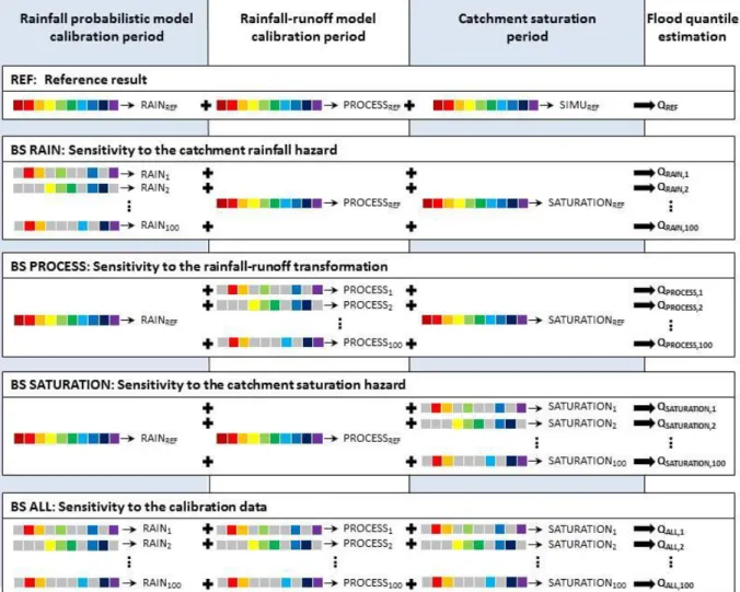
The methodology used aims at quantifying the sensitivity of the SCHADEX method to observed hydroclimatic variability. As stated in section 1, the sensitivity will be firstly assessed for each model constituting the SCHADEX method using independent block-bootstrap experiments (noted ‘‘BS’’ hereafter), and then for all models by a general bootstrap experiment. The general methodology used is illustrated in Figure 1. It consists of five parts:
1. Definition of a reference SCHADEX result (noted ‘‘REF’’) for each catchment, using a probabilistic rainfall model and a rainfall-runoff model calibrated over all the available data and using the entire available period of record as the simulation period.
2. Quantification of the sensitivity of the SCHADEX flood estimation to the use of 100 different rainfall probabilistic models (‘‘BS RAIN’’ experiment), calibrated over 100 different subperiods.
3. Quantification of the sensitivity of the SCHADEX flood estimations to the use of 100 different rainfall-runoff model parameter sets (‘‘BS PROCESS’’ experiment), calibrated over 100 different subperiods. Note that bootstrap procedures, widely employed in statistical characterization of uncertainty and sensitivity analysis, have been also recently used for calibration of rainfall-runoff models. Thus, Ebtehaj et al. [2010] and Selle and Hannah [2010] show that block-bootstrap allows robust estimations of rainfall-runoff model parameter sets.
4. Quantification of the sensitivity of the SCHADEX flood estimations to the use of 100 different subperiods as simulation periods (‘‘BS SATURATION’’ experiment).
Page 7 on 28
5. Quantification of the most sensitive parameters of the SCHADEX method by using 100 different subperiods as calibration periods for the rainfall probabilistic model and for the rainfall-runoff model and as simulation periods (‘‘BS ALL’’ experiment).
FIGURE 1:
2.2.2 Generation of Subperiods Through 1 Year Block-Bootstrapping Method
For each block of the four bootstrap experiments performed, 100 subperiods of 25 years are generated. Blocks are constituted by assembly single hydrological years, thus keeping the inter-annual autocorrelation of temperature, precipitation, and streamflow series. Nevertheless, the long-term hydroclimatic autocorrelation is not preserved in this approach. For example, long-dry periods which slowly dry up catchment groundwater (typically comprising five or more continuous years) are broken into several non-sequential years in the approach. Note that no replacements have been allowed, meaning that each observed year does not appear more than once in each generated sub-period. The choice of sub-periods length (25 years hereafter) is a subjective choice, made on a trade-off between (i) having long enough calibration periods for an efficient constrain of the model parameters and (ii) having short enough sub-periods for examining climatically contrasted sub-periods. Feedback from the 80 SCHADEX studies performed in France over the last 6 years indicates that 25 years of (good quality) data is an appropriate data length required for reliable extreme flood estimates using the SCHADEX method [Paquet et al., 2012, 2013].
3 DATA
3.1 Catchments Set and Available Data
Six catchments have been studied: three French catchments (the Corrèze river at Brive-la-Gaillarde, the Tarn river at Millau, the Romanche river at Champeau), one Austrian catchment (the Kamp river at Zwettl), one Canadian catchment (the Coquitlam river at the Coquitlam Dam), and one Norwegian catchment (the Atna river at Atnasjø). These catchments are small to medium, with area ranging from 188 to 2170 km². Table 1 presents several characteristics of each catchment, described by three daily series: natural streamflow at the outlet, areal precipitation, and areal temperature. The lengths of the different observed series are given in Table 1. Hydrological regimes are illustrated for each catchment in Figure 2. The principle flood-driving mechanisms of each catchment are detailed in the following:
1. The high streamflows of the Atna river at Atnasjø occur particularly during the late spring and early summer reflecting the melting of the seasonal snowpack, with the largest flooding events occurring due to heavy precipitation during this period. The Atna river at Atnasjø is also subject to peak flows resulting primarily from heavy rainfall (although snowmelt can also make a minor contribution) during the late summer and autumn periods.
2. The highest streamflows of the Romanche river at Champeau occurs equally during the melting period which is starting in April and is reaching a maximum in June. Rainfall events are generating floods during this high base-flow period. Finally, floods also occur during autumn and arise from heavy rainfall events.
3. The periods of highest streamflow in the Coquitlam river at the Coquitlam Dam coincide with the heavy winter rainfall events (from October to March) at which time the air temperature may be above freezing at all altitudes in the catchment. These floods may thus be produced by combination of intense rainfall and snowmelt.
4. Floods are occurring during two different periods for the Corrèze river at Brive-la-Gaillarde: the October-March period where rainfall events are mainly generated by oceanic circulations and the April-July period where rainfall events are mainly generated by South circulations.
5. The Tarn river at Millau is subject to intense floods generated by heavy rainfall events which mainly occur from late September to May and, more particularly, from October to January.
6. Finally, the periods of highest streamflows in the Kamp river at Zwettl is in spring, but high floods are also observed during summer (from July to August), generated by heavy rainfall events.
Page 8 on 28
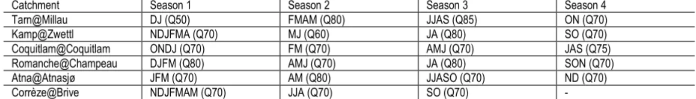
An analysis of the rainfall hazard seasonality has been made for each catchment, in order to group months with similar rainfall hazard in three or four seasons per catchment, typically. Seasonal subsamples of rainfall events are then constituted for the definition of a MEWP distribution. The seasonal splitting chosen for each catchment is shown in Table 2. For example, the season 1 of the Atna at Atnasjø catchment is constituted by the January, the February, and the March months. A last sampling step is performed for each seasonal WP subsamples: heavy rainfall events are identified for estimating the scale parameter values of each seasonal WP subsamples by fitting an exponential law. The quantile thresholds considered for the definition of the heavy rainfall event subsamples are also indicated in Table 2. For example, the season 1 heavy rainfall event subsample of the Atna at Atnasj catchment is constituted by the rainfall events greater than the 0.70 quantile value.
TABLE 1 FIGURE 2
TABLE 2
3.2 WP Classifications
Four different WP classifications previously defined have been used for this study as a basis for MEWP model definition:
1. Eight French WPs [Garavaglia et al., 2010] have been used for the three French catchments. 2. Five Austrian WPs [Brigode et al., 2013b] have been used for the Austrian catchment.
3. Five Coastal British Columbia WPs [Brigode et al., 2013c] have been used for the Canadian catchment. 4. Four Norwegian WPs [Fleig, 2011] have been used for the Norwegian catchment.
The spatial coverage of the rainfall stations used for the definition of the four regional weather pattern classifications is illustrated in the Figure 2.
4 RESULTS
The results are presented separately for the four block-bootstrap experiments: (i) flood estimations performed by using different sub-periods as input to the rainfall probabilistic model (BS RAIN), (ii) flood estimations performed by using different sub-periods as the calibration period for the rainfall-runoff model (BS PROCESS), (iii) flood estimations performed by using different sub-periods as the simulation period (BS SATURATION), and (iv) flood estimations performed by using different sub-periods as input of the rainfall probabilistic model, of the rainfall-runoff model and as simulation period (BS ALL).
4.1 BS RAIN Experiment
Figure 3 presents the 100 extreme rainfall estimations performed with the rainfall probabilistic model calibrated over 100 different sub-periods for each of the six catchments. These estimates are compared with the reference rainfall estimates (performed using the entire record period as calibration period of the rainfall probabilistic model, plotted with orange lines) and with the annual maximum 24h rainfall observations, plotted with blue crosses. The distributions of the 100 rainfall estimates are summarized at three particular return periods (10 year, 100 year, and 1000 year) with violin plots (plotted with black contours). BS RAIN experiment results show that the rainfall estimations are sensitive to the sub-periods used for calibration of the rainfall probabilistic model. Thus, extreme rainfall estimation ranges are significant for all of the six catchments considered, and the spread in the 100 estimations is particularly large for the Tarn at Millau, the Kamp at Zwettl, and the Corrèze at Brive-la-Gaillarde catchments. The 100 estimations are generally distributed around the reference estimations. However, the median values of the 100 BS RAIN estimations (represented with black points on the violin plots for the three particular return periods) are higher than reference estimations for all catchments except for the Tarn river at Millau catchment (where the median BS RAIN values are similar to the reference estimations) and the Atna river at Atnasjø catchment (where the median BS RAIN values are lower than the reference estimations). BS RAIN estimations over the Kamp catchment at Zwettl are rather particularly distributed. This is due to the presence or absence of the 2002 year within the sub-periods used as calibration of the rainfall probabilistic model, since the
Page 9 on 28
August 2002 event is a major ‘‘outlier’’ in the observed distribution. The outlier term reflects an event with a much larger magnitude than other observed heavy precipitation events and which could belong to a different probabilistic distribution (see discussion about ‘‘dragon king’’ terminology in Sornette and Ouillon [2012 for example). Finally, rainfall probabilistic model calibrated over a sub-period containing the year 2002 leads to extreme rainfall estimations which are significantly higher than values estimated with a rainfall probabilistic model calibrated without the year 2002. There are also other cases, for example Atna river at Atnasjø and Corrèze river at Brive-la-Gaillarde for which some of the highest observed rainfall values lie outside the envelope of simulated estimates, although the discrepancies are not as large as those observed for the Kamp catchment.
FIGURE 3
Figure 4 presents the 100 extreme flood estimations performed with rainfall probabilistic model calibrated over 100 different sub-periods, with the reference rainfall-runoff model parameter set and the reference simulation period for each of the six catchments. Each of these simulations is compared with the reference estimations (plotted with orange lines) and with annual maximum 24h streamflow observations (plotted with blue crosses). The distributions of the 100 BS RAIN simulations are summarized at three particular return periods (10 year, 100 year, and 1000 year) with violin plots (plotted with black contours). Since only the rainfall probabilistic model considered differs between the 100 flood estimations performed in the BS RAIN experiment, comments on the obtained BS RAIN flood estimations are the same as those previously made for BS RAIN rainfall estimations: BS RAIN experiment results show that the extreme flood estimations are sensitive to the sub-periods used for calibration of the rainfall probabilistic model. Thus, extreme flood estimation ranges are significant for all of the six catchments considered, and the spread in the 100 estimations is particularly large for the Tarn at Millau, the Kamp at Zwettl, and the Corrèze at Brive-la-Gaillarde catchments.
FIGURE 4
Table 3 describes the relationship between chosen rainfall probabilistic model parameters and the estimated 1000 year return period streamflow values (noted Q1000 hereafter) in order to understand which rainfall
probabilistic model parameter is driving the extreme flood estimations. For each catchment, the Spearman correlation obtained between the 100 values of Q1000 and the scale parameter values obtained over each WP for
the one particular season (parameter k of the equation (1)). The season considered is, for each catchment, the ‘‘season-at-risk one’’ (i.e., the season where the intensity of heavy rainfall events is the highest). For the Tarn at Millau, the Kamp at Zwettl, the Atna at Atnasjø catchment, and the Corrèze at Brive-la-Gaillarde catchments, the Q1000 estimated values are strongly dependent to the scale parameter values of one particular WP. Q1000
estimated values of the Tarn at Millau and Corrèze at Brive-la-Gaillarde catchments are strongly dependent to the seasonal values of the French WP4 scale parameter values, with Spearman correlation of 0.96 and 0.92, respectively. This particular WP is a typical Mediterranean circulation known to be responsible of heavy rainfall events over South-Eastern part of France [Garavaglia et al., 2010]. Q1000 estimated values of the Kamp at Zwettl
catchment are strongly dependent on the seasonal value of the Austrian WP2 scale parameter values, with Spearman correlation of 0.96. This particular WP is a ‘‘continental depression’’ situation which brings rainy days over the eastern part of Austria [Brigode et al., 2013b]. For the Kamp catchment at Zwettl, an analysis of major rainy events (August 1985 and August 2002) reveals that all the major historical events belong to Austrian WP2 [Brigode et al., 2011]. Rainfall hazard in this catchment seems thus to be totally driven by the magnitude of WP2 events. Finally, the central role of the August 2002 event (coherently belonging to the Austrian WP2) for the characterization of the rainfall hazard highlighted in Figures 3 and 4 is confirmed: sub-periods without the year 2002 lead to lower WP2 scale parameter values and thus lower extreme rainfall estimations and lower extreme flood estimations. Q1000 estimated values of the Atna at Atnasjø catchment are strongly dependent on the
seasonal value of the Norwegian WP2 scale parameter values, with Spearman correlation of 0.99. This particular WP regroups days which are particularly rainy in Sweden and in the South-eastern part of Norway. The dependence from Q1000 estimated values to seasonal scale parameter values of each WP is less clear for the two
other catchments. Finally, these four catchments have a heavy rainfall hazard characterized by one particular synoptic genesis, which is the French WP4, the Austrian WP2, the Norwegian WP2, and the French WP4 for the Tarn at Millau, the Kamp at Zwettl, the Atna at Atnasjø catchment, and the Corrèze at Brive-la-Gaillarde catchments, respectively. For the Romanche at Champeau catchment, the scale parameter values are less contrasted between the different French WPs, with a strongest link with WP2 scale parameter values (Spearman correlation of 0.68). For the Coquitlam catchment at the Coquitlam Dam, highest Q1000 estimated values seem to
Page 10 on 28
0.51, 0.41, and 0.38, respectively). These two catchments are thus characterized by a rainfall hazard generated by different type of synoptic situations.
The same analysis (not shown here) has been performed for the other seasons and for another rainfall probabilistic parameter, the Central Rainfall event probability of occurrence of each WP. It reveals that extreme rainfall estimations (and thus extreme flood estimations) are not significantly influenced by the variability of the Central Rainfall event probability of occurrence of each WP. The scale parameter values of the ‘‘season-at-risk’’ and of the ‘‘WPat-risk’’ are thus clearly the driver of extreme flood estimations within the BS RAIN experiment.
TABLE 3
4.2 BS PROCESS Experiment
Figure 5 summarizes the NSE (top graph) and NSECDF (bottom graph) performances obtained by the 100 BS
PROCESS parameter sets (colored boxplots) and obtained by the reference parameter sets (orange points) for the six studied catchments. These scores are estimated over the entire record period of each catchment and are thus calibration scores for the reference parameter sets. The MORDOR model shows good general performance over the different catchments, with all NSE values over 0.7. The variability of the 100 performances values obtained with the 100 BS PROCESS parameter sets for each catchment is limited, expect for the Kamp at Zwettl catchment.
FIGURE 5
Figure 6 presents the 100 extreme flood estimations performed with the rainfall-runoff model calibrated over 100 different subperiods for each of the six catchments. Each of these simulations is compared with the reference flood estimations (plotted with orange lines) and with annual maximum 24 h streamflow observations (plotted with blue crosses). The distributions of the 100 BS PROCESS simulations are summarized at three particular return periods (10 year, 100 year, and 1000 year) with violin plots (plotted with black contours). The BS PROCESS experiment results show that the extreme flood estimations are sensitive to the sub-periods used as calibration of the rainfall-runoff model. Thus, extreme flood estimation ranges are important for the six catchments considered. The 100 estimations are distributed around the reference estimation, which are represented with black points on the violin plots for the three particular return periods. BS PROCESS estimations over the Kamp catchment at Zwetll and over the Atna river at Atnasjø, have especially wide distributions at the larger return periods. Several rainfall-runoff model calibrations for these two catchments produce extreme streamflow estimations which are significantly outside of range of the majority of extreme streamflow estimations.
FIGURE 6
Figure 7 describes differences between the 100 rainfall-runoff model calibrations for each catchment. Since it is impossible to interpret model parameter values for such conceptual models with numerous calibrated parameters, the comparison has been made directly on simulated streamflow. More specifically, extreme flood estimation values have been linked for each catchment to rainfall-runoff simulations of the biggest observed flood. For each catchment, the 100 rainfall-runoff model parameter sets identified within the BS PROCESS experiment have been used for simulating the day corresponding to the highest observed event (i.e., one particular day is selected for each catchment, independent of which calibration years are taken). These streamflow simulated values are noted QSIM hereafter, while the streamflow simulated values simulated using the reference rainfall-runoff model
parameter sets are noted QSIMREF hereafter. The highest observed events are the 5 November 1994 for the Tarn
river at Millau, the 8 August 2002 for the Kamp river at Zwettl, the 31 October 1981 for the Coquitlam river at Coquitlam, the 22 September 1968 for the Romanche river at Champeau, the 1 June 1995 for Atna river at Atnasjø, and the 4 October 1960 for the Corrèze river at Brive-la-Gaillarde. Figure 7 thus presents, for each catchment, the 100 ratios between Q1000 streamflow values obtained within the BS PROCESS experiment and the
reference Q1000REF values (y axis) against the 100 ratios between the QSIM values simulated for the particular day
corresponding to the highest observed event and QSIMREF values simulated for the same day by the reference
rainfall-runoff model parameter set (x axis). Finally, the red points highlight the parameter sets obtained by calibration on sub-periods which contain the highest observed events, while black points highlight the parameter sets obtained by calibration on sub-periods which do not contain the highest observed events. A clear relationship between the highest Q1000 estimations and the highest values of simulated annual streamflow maxima is observed
for the Kamp river at Zwettl, the Coquitlam at the Coquitlam Dam, the Romanche at Champeau, and the Corrèze at Brive-la-Gaillarde catchments. For these four catchments, the highest Q1000 values are estimated by
rainfall-Page 11 on 28
runoff model parameter sets which are simulating particularly high values of the highest observed streamflow values, compared to the other 100 simulations. No clear relationship between the two variables considered is observed for the Tarn river at Millau and the Atna river at Atnasjø. It is important to note that the relative variability of the Q1000 estimated values are different within the different catchments, as highlighted by the Figure 7: the
differences between the minimum and the maximum Q1000 values are particularly large for the Kamp at Zwetll
catchment and the Atna at Atnasjø catchment. Interestingly, for the Kamp at Zwettl catchment, the highest Q1000
values are estimated by rainfall-runoff model calibrated on sub-periods which are not containing the 2002 year and thus the August 2002 events.
Note that numerous indicators have been tested in order to link hydroclimatic characteristics of the 100 calibration periods and the 100 different flood estimations of the BS PROCESS experiment: mean precipitation values of the calibration periods, aridity index of the calibration periods, number of observed floods within the calibration periods, intensity of observed floods within the calibration periods, etc. Nevertheless, no clear relationship has been observed between these indicators and the extreme flood estimations. Thus, it is straightforward that a rainfall-runoff model simulating high streamflow values for the highest flood observations is then producing high extreme flood estimations, but understanding which hydroclimatic characteristic of the rainfall-runoff model is conditioning the extreme flood estimation seems to be a difficult task.
FIGURE 7
4.3 BS SATURATION Experiment
Figure 8 presents the 100 flood estimations performed with 100 different subperiods as simulation periods for each of the six catchments. Each of these simulations is compared with the reference flood estimations (plotted with orange lines) and with annual maximum 24h streamflow observations (plotted with blue crosses). The distribution of the 100 BS SATURATION simulations is summarized at three particular return periods (10 year, 100 year, and 1000 year) with violin plots (plotted with black contours). The BS SATURATION experiment results indicate that the extreme flood estimations are insensitive to the sub-periods used as simulation periods for the catchments considered. The lack of a significant spread in the estimations is similar for all of the catchments, and contrasts quite strongly with Figures 4 and 6.
FIGURE 8
4.4 Comparison of the SCHADEX Model Sensitivities
Figure 9 presents a comparison of Q1000 values estimated by the three BS experiment and the reference flood
estimations for each catchment. For the six catchments, the variability generated by the use of different simulation periods (BS SATURATION) does not imply a significant variability in the extreme flood estimations. Nevertheless, the use of different subperiods as calibration period for the rainfall probabilistic model (BS RAIN) and the rainfallrunoff model (BS PROCESS) induces a large variability in the Q1000 estimations for the six
catchments considered. The variability in the Q1000 estimations is higher for the BS RAIN experiment than for the
BS PROCESS experimentand is particularly large for the rainfall-driven catchments (the Tarn at Millau, the Kamp at Zwettl, and the Corrèze at Brive-la-Gaillarde catchments). Note that the median of the BS RAIN estimations are higher that reference estimations (REF) for all catchments except for the Tarn river at Millau catchment, unlike for the median of the BS PROCESS estimations, which are higher for two catchments (the Kamp at Zwettl and the Romanche at Champeau catchments) and lower for the other four catchments (the Tarn at Millau, the Coquitlam at Coquitlam, the Atna at Atnasjø, and the Corrèze at Brive-la-Gaillarde catchments). In conclusion, the observed hydro-meteorological variability is strongly influencing the extreme streamflow estimations through the sensitivity of the rainfall probabilistic model and of the rainfall-runoff model to their calibration periods.
FIGURE 9
4.5 BS ALL Experiment
Figure 10 presents the BS ALL experiment results showing the 100 Q1000 values estimated against the 100 scale parameters of the rainfall probabilistic model estimated as the drivers of rainfall hazard for each catchment in Table 3. Moreover, the QSIM/QSIMREF ratios (estimated as for the BS PROCESS experiment) of the BS ALL
Page 12 on 28
link between Q1000 estimations and rainfall probabilistic model, while the color gradients are indicators of the link
between Q1000 estimations and rainfall-runoff model. The influence of the scale parameter values of the
‘‘WP-at-risk’’ is clearly highlighted, especially for the rainfall-dominated catchments where a particular WP is critical and clearly driving the rainfall hazard: the Tarn river at Millau, the Kamp river at Zwettl, and the Corrèze at Brive-la-Gaillarde catchments. For these catchments, the highest Q1000 values are estimated when a sub-period with high
‘‘WP-at-risk’’ scale parameters values are considered. Even if several WPs appeared to be responsible for heavy rainfall events over the Coquitlam river at Coquitlam (line 3 of the Table 3), values of the Coastal BC WP3 scale parameter seem to be linked with Q1000 estimated values. For the Atna and the Romanche rivers, the influence of
the critical WPs on the BS ALL Q1000 estimations is less clear. The influence of the rainfall-runoff model is not
straightforward for the six studied catchments. For the Tarn at Millau and the Coquitlam at Coquitlam catchments, no significant influence of the rainfall-runoff model calibration on the Q1000 estimation is found. For the Atna at
Atnasjø catchment, the lowest Q1000 estimated values seem to be due to rainfall-runoff model parameter sets
which are simulating particularly low values of the highest observed streamflow values, regarding to the other simulations (the lowest points are colored in blue). For the Romanche at Champeau catchment, the role of the rainfall-runoff model parameter sets is not clear. Finally, the Kamp at Zwettl and the Corrèze at Brive-la-Gaillarde catchments BS ALL results reveal interesting influence limits of the rainfall-runoff model: it seems that the higher the scale parameter values of the WP-at-risk is, the less important the rainfall-runoff parameter set is. Thus, for the Corrèze at Brive-la-Gaillarde catchment, the extreme flood estimations characterized by scale parameter values higher than the reference value are not influenced by the rainfall-runoff model calibration. Conversely, the extreme flood estimations characterized by scale parameter values lower than the reference value are influenced by the rainfall-runoff model calibration: the highest Q1000 values are estimated by rainfall-runoff model parameter
sets which are simulating particularly high values of the highest observed streamflow values. Finally, for the Kamp at Zwettl catchment, the extreme flood estimations characterized by scale parameter values higher than the reference value are simulations performed considering the August 2002 event, while other simulations are not considering this event within the calibration period.
FIGURE 10
5 CONCLUSIONS
A new methodology has been developed in order to quantify the sensitivity of extreme flood estimations to observed hydro-climatological variability, based on block-bootstrap techniques. Since the extreme flood estimations are performed through an event-based stochastic flood simulation approach, the methodology proposed is based on the three-part decomposition of the flood-producing factors inferred by such methods: the sensitivity of extreme flood estimations to the rainfall hazard, to the catchment saturation hazard and to the rainfall-runoff transformation are quantified. This new methodology is thus able to define to which part of an event-based continuous flood simulation method the final results (estimation of extreme streamflow) are most sensitive. An application of this methodology is done on six different catchments using the SCHADEX method. The application of the methodology to six catchments with different characteristics shows that observed hydro-climatological variability influences the extreme flood estimations. First, the parameters of the rainfall probabilistic model strongly influence the extreme streamflow estimation. For a given catchment, SCHADEX flood estimations are indeed highly driven by the scale parameter values of the ‘‘WP-at-risk’’ of the ‘‘season-at-risk.’’ These parameters are thus indicators of the heavy rainfall driving processes. It is interesting to note that these indicators are different for each catchment: some catchments have a heavy rainfall hazard characterized by one particular synoptic genesis (the French WP4 for the Tarn at Millau and the Corrèze at Brive-la-Gaillarde catchments, the Austrian WP2 for the Kamp at Zwettl catchment and the Norwegian WP2 for the Atna at Atnasjø catchment), while other catchments have a heavy rainfall hazard generated by different types of synoptic situations (the Coquitlam at Coquitlam and the Romanche at Champeau catchments). This observation could be particularly important for studying climate change impacts on heavy rainfall events, since the heavy rainfall producing processes could be identified over each catchment and thus be particularly studied.
The rainfall-runoff model parameters, which depend on the climate variability of the period chosen for the parameter calibration, also significantly influence the results. Considering that rainfall-runoff model parameter set values and rainfall-runoff model internal variables are non-explainable for such types of conceptual rainfall-runoff model, it has been chosen to characterize each parameter set in terms of its rainfall-runoff simulation of the biggest observed flood event, for each catchment. It appears that the parameter sets which simulated particularly
Page 13 on 28
high values for the biggest observed flood event compared to the other simulated values are responsible for the highest values of extreme flood estimations. Note that numerous indicators have been tested in order to link the hydro-climatic characteristics of the rainfall-runoff model calibration periods with the different flood estimations (mean precipitation values of the calibration periods, aridity index of the calibration periods, number of observed floods within the calibration periods, intensity of observed floods within the calibration periods, etc.), but no clear relationship has been observed between any of these indicators and the extreme flood estimations. It is thus hard to identify specific climatic conditions within the calibration period which are most responsible for this sensitivity. The catchment saturation conditions, simulated in the SCHADEX framework through the rainfall-runoff model fed by different simulation sub-periods, have significantly less influence on extreme flood estimations than rainfall hazard and rainfall-runoff transformation. Thus, it seems that the patterns of catchment saturation do not vary significantly between the sampled sub-periods. This observation could be an artifact of the block-bootstrap sampling methodology used in some cases since autocorrelation greater than one hydrological year is not preserved. However, this would only be relevant in strongly groundwater-dominated catchments.
The general sensitivity analysis highlights the rainfall hazard as the first explaining factor of the extreme flood estimation variability obtained, especially for rainfall-driven catchments. The extreme flood estimation is thus most sensitive to the variability of observed rainfall hazard than to the variability of catchment saturation hazard or differences of rainfall-runoff transformations. These observations may be not true for lower and median flood events (analysis not performed in this study). Thus, Merz and Blöschl [2009] highlighted, by a correlation analysis of statistical flood moments, that flood runoff is on average more strongly controlled by the catchment saturation condition than by the rainfall hazard. Thus, a shift in flood-controlling factors seems to exist: the catchment saturation conditions are important for lower and median floods, while the additional rainfall amount is the only driving factor for extreme flood events.
Understanding which process is responsible for the differences in the extreme flood estimations for different rainfall-runoff model calibration periods seem to be the most challenging and interesting question raised by this study. Is it the number of observed floods or the intensity of the observed floods which are conditioning the extreme flood simulation characteristics of the rainfall-runoff model and thus the final extreme flood estimations? Does the rainfall-runoff model need to have observations of particular flood-producing processes within the calibration period for being better constrained for flood simulations? These questions will be investigated more closely in future works. Similarly, finding signatures which describe the ‘‘flood-producing’’ characteristics of a given sub-period could be investigated more closely in the future.
An important point raised by this study is the dominating role played by outliers within the observed records for extreme flood estimations. To this regard, the Kamp at Zwettl catchment is a very interesting case study, since the presence of the August 2002 ‘‘dragon-king’’ event [Sornette and Ouillon, 2012 terminology] within the calibration period of the probabilistic rainfall model or of the rainfall-runoff model is driving the final extreme flood estimations: calibration sub-periods containing this event lead to higher extreme flood estimations than those estimated without consideration of this event within the calibration sub-periods. Viglione et al. [2013] used this case study to illustrate the weight of one event (August 2002) on flood frequency analysis and how this weight is reduced when additional information (e.g., temporal, spatial, and causal information) are combined and used for flood estimations.
Note that the proposed methodology is not able to take into account the long-term memory of catchment to long periods of dryness or wetness. These sub-periods could significantly influence the flood magnitudes and flood frequency [Pathiraja et al., 2012]. The application of the Generalised Split Sample Test developed by Coron et al. [2012] in order to fully quantify the sensitivity of the simulated streamflow to the calibration periods used is an interesting idea. Finally, this general methodology could be applied on several other catchments in order to generalize the obtained conclusions.
This sensitivity analysis provides a basis for the understanding of the major factors influencing the frequency of occurrences and the magnitudes of flood events of each considered catchment. Moreover, these results are important for climate change impact studies on extreme floods. In particular, the focus on the future evolution of climate variables will be put on the most relevant parameters (the scale parameters describing heavy rainfall hazard for example), instead of a general description of future scenarios.
Acknowledgments. The authors thank Alberto Viglione and an anonymous reviewer who provided constructive
Page 14 on 28
6 REFERENCES
Arnaud, P., and J. Lavabre (1999), Nouvelle approche de la prédétermination des pluies extrêmes, C. R. Acad. Sci., Ser. IIa, 328(9), 615–620, doi:10.1016/S1251–8050(99)80158-X.
Bernardara, P., C. De Michele, and R. Rosso (2007), A simple model of rain in time: An alternating renewal process of wet and dry states with a fractional (non-Gaussian) rain intensity, Atmos. Res., 84(4), 291–301, doi:10.1016/j.atmosres.2006.09.001.
Beven, K., and A. Binley (1992), The future of distributed models: Model calibration and uncertainty prediction, Hydrol. Processes, 6(3), 279–298, doi:10.1002/hyp.3360060305.
Blazkova, S., and K. Beven (2002), Flood frequency estimation by continuous simulation for a catchment treated as ungauged (with uncertainty) Water Resour. Res., 38(8), 1139, doi:10.1029/2001WR000500.
Boughton, W., and O. Droop (2003), Continuous simulation for design flood estimation—A review, Environ. Modell. Software, 18(4), 309–318, doi:10.1016/S1364–8152(03)00004–5.
Bradley, A. A., and K. W. Potter (1992), Flood frequency analysis of simulated flows, Water Resour. Res., 28(9), 2375–2385, doi:10.1029/92WR01207.
Brigode, P., P. Bernardara, E. Paquet, J. Gailhard, P. Ribstein, and R. Merz (2011), Complete application of the SCHADEX method on an Austrian catchment: Extreme flood estimation on the Kamp river, Geophys. Res. Abstr., 14, 6771.
Brigode, P., P. Bernardara, J. Gailhard, F. Garavaglia, P. Ribstein, and R. Merz (2013a), Optimization of the geopotential heights information used in a rainfall-based weather patterns classification over Austria, Int. J. Climatol., 33(6), 563–1573, doi:10.1002/joc.3535.
Brigode, P., Z. Mićović, P. Bernardara, E. Paquet, F. Garavaglia, J. Gailhard, and P. Ribstein (2013b), Linking ENSO and heavy rainfall events over Coastal British Columbia through a weather pattern classification, Hydrol. Earth Syst. Sci., 17(4), 1455–1473, doi:10.5194/hess-17–1455-2013.
Brigode, P., L. Oudin, and C. Perrin (2013c), Hydrological model parameter instability: A source of additional uncertainty in estimating the hydrological impacts of climate change?, J. Hydrol., 476, 410–425, doi:10.1016/j.jhydrol.2012.11.012.
Calver, A., and R. Lamb (1995), Flood frequency estimation using continuous rainfall-runoff modelling, Phys. Chem. Earth, 20(5–6), 479–483, doi:10.1016/S0079–1946(96)00010-9.
Cameron, D., K. Beven, J. Tawn, and P. Naden (1999), Flood frequency estimation by continuous simulation (with likelihood based uncertainty estimation), Hydrol. Earth Syst. Sci., 4(1), 23–34, doi:10.5194/hess-4–23-2000. Choi, H. T., and K. Beven (2007), Multi-period and multi-criteria model conditioning to reduce prediction uncertainty in an application of TOPMODEL within the GLUE framework, J. Hydrol., 332(3–4), 316–336, doi:10.1016/j.jhydrol.2006.07.012.
Coron, L., V. Andréassian, C. Perrin, J. Lerat, J. Vaze, M. Bourqui, and F. Hendrickx (2012), Crash testing hydrological models in contrasted climate conditions: An experiment on 216 Australian catchments, Water Resour. Res., 48,W05552, doi:10.1029/2011WR011721.
Cowpertwait, P. S. P. (1995), A generalized spatial-temporal model of rainfall based on a clustered point process, Proc. R. Soc. London, Ser. A, 450(1938), 163–175, doi:10.1098/rspa.1995.0077.
Delgado, J. M., H. Apel, and B. Merz (2010), Flood trends and variability in the Mekong river, Hydrol. Earth Syst. Sci., 14(3), 407–418, doi: 10.5194/hess-14–407-2010.
Ebtehaj, M., H.Moradkhani, and H. V. Gupta (2010), Improving robustness of hydrologic parameter estimation by the use of moving block bootstrap resampling, Water Resour. Res., 46, W07515, doi:10.1029/2009WR007981. Efron, B. (1979), Bootstrap methods: Another look at the Jackknife, Ann. Stat., 7(1), 1–26, doi:10.1214/aos/1176344552.
Fleig, A. (2011), Definition of weather patterns for extreme rainfall analysis over Norway, Scientific Report of the Short Term Scientific Mission. AQ1
Page 15 on 28
Franchini, M., K. R. Helmlinger, E. Foufoula-Georgiou, and E. Todini (1996), Stochastic storm transposition coupled with rainfall-runoff modeling for estimation of exceedance probabilities of design floods, J. Hydrol., 175(1), 511–532, doi:10.1016/S0022–1694(96)80022-9.
Franchini, M., A. M. Hashemi, and P. E. O’Connell (2000), Climatic and basin factors affecting the flood frequency curve: PART II A full sensitivity analysis based on the continuous simulation approach combined with a factorial experimental design, Hydrol. Earth Syst. Sci., 4(3), 483–498, doi:10.5194/hess-4–483-2000.
Franks, S. W., and G. Kuczera (2002), Flood frequency analysis: Evidence and implications of secular climate variability, New South Wales, Water Resour. Res., 38(5), 1062, doi:10.1029/2001WR000232.
Fréchet, M. (1927), Sur la loi de probabilité de l’écart maximum, Ann. Soc. Polonaise Math., 6, 92–116.
Gan, T. Y., and S. J. Burges (1990), An assessment of a conceptual rainfall-runoff models ability to represent the dynamics of small hypothetical catchments, 2: Hydrologic responses for normal and extreme rainfall, Water Resour. Res., 26(7), 1605–1619, doi:10.1029/WR026i007p01605.
Garavaglia, F. (2011), Méthode SCHADEX de prédétermination des crues extrêmes.Méthodologie, applications et études de sensibilité, PhD thesis, Univ. de Grenoble.
Garavaglia, F., J. Gailhard, E. Paquet, M. Lang, R. Garc¸on, and P. Bernardara (2010), Introducing a rainfall compound distribution model based on weather patterns sub-sampling, Hydrol. Earth Syst. Sci., 14(6), 951–964, doi:10.5194/hess-14–951-2010.
Garavaglia, F., M. Lang, E. Paquet, J. Gailhard, R. Garçon, and B. Renard (2011), Reliability and robustness of rainfall compound distribution model based on weather pattern sub-sampling, Hydrol. Earth Syst. Sci., 15(2), 519–532, doi:10.5194/hess-15–519-2011.
Garçon, R. (1999), Modèle global pluie-débit pour la prévision et la prédétermination des crues, La Houille Blanche, 7–8, 88–95, doi: 10.1051/lhb/1999088.
Gumbel, E. J. (1958), Statistics of Extremes, Columbia Univ. Press, New York.
Hashemi, A. M., M. Franchini, and P. E. O’Connell (2000), Climatic and basin factors affecting the flood frequency curve: PART I-A simple sensitivity analysis based on the continuous simulation approach, Hydrol. Earth Syst. Sci., 4(3), 463–482, doi:10.5194/hess-4–463-2000.
Hingray, B., and A. Mezghani (2008), Utilisation des réanalyses NCEP pour la génération de scénarios météorologiques. Application pour la génération de scénarios de crues pour le Rhône à l’amont du Leman, La Houille Blanche, 6, 104–110, doi:10.1051/lhb:2007090.
Klemeš, V. (2000a), Tall tales about tails of hydrological distributions. I, J. Hydrol. Eng., 5(3), 227–231. Klemeš, V. (2000b), Tall tales about tails of hydrological distributions. II, J. Hydrol. Eng., 5(3), 232–239.
Lamb, R. (1999), Calibration of a conceptual rainfall-runoff model for flood frequency estimation by continuous simulation, Water Resour. Res., 35(10), 3103–3114, doi:10.1029/1999WR900119.
Le Lay, M., S. Galle, G. M. Saulnier, and I. Braud (2007), Exploring the relationship between hydroclimatic stationarity and rainfall-runoff model parameter stability : A case study in West Africa, Water Resour. Res., 43, W07420, doi:10.1029/2006WR005257.
Lennartsson, J., A. Baxevani, and D. Chen (2008), Modelling precipitation in Sweden using multiple step Markov chains and a composite model, J. Hydrol., 363(1–4), 42–59, doi:10.1016/j.jhydrol.2008.10.003.
Li, Z., F. Brissette, and J. Chen (2012), Finding the most appropriate precipitation probability distribution for stochastic weather generation and hydrological modeling in Nordic watersheds, Hydrol. Processes, 27, 3718– 3729, doi:10.1002/hyp.9499.
Merz, B., and A. H. Thieken (2005), Separating natural and epistemic uncertainty in flood frequency analysis, J. Hydrol., 309(1–4), 114–132, doi:10.1016/j.jhydrol.2004.11.015.
Merz, R., and G. Blöschl (2008a), Flood frequency hydrology: 1. Temporal, spatial, and causal expansion of information, Water Resour. Res., 44, W08432, doi:10.1029/2007WR006744.