Non-Gaussian spatiotemporal simulation of multisite daily precipitation: downscaling framework.

1 1

Non-Gaussian spatiotemporal simulation of multisite daily

precipitation: downscaling framework

4

5

M. A. Ben Alaya1, T.B.M.J. Ouarda3, 2 and F. Chebana2

6 7

1

Pacific Climate Impacts Consortium, University of Victoria,

8

PO Box 1700 Stn CSC, Victoria, BC V8W2Y2, Canada

9 10

2

INRS-ETE, 490 rue de la Couronne, Québec (QC),

11

Canada G1K 9A9

12 13

3

Masdar Institute of science and technology

14

P.O. Box 54224, Abu Dhabi, UAE

15 16

17

18 *

Corresponding author: mohamedalibenalaya@uvic.ca 19 20 21 2017-01-23 22 23

2 Abstract:

24

Probabilistic regression approaches for downscaling daily precipitation are very useful.

25

They provide the whole conditional distribution at each forecast step to better represent

26

the temporal variability. The question addressed in this paper is: How to simulate

27

spatiotemporal characteristics of multisite daily precipitation from probabilistic

28

regression models? Recent publications point out the complexity of multisite properties

29

of daily precipitation and highlight the need for using a non-Gaussian flexible tool. This

30

work proposes a reasonable compromise between simplicity and flexibility avoiding

31

model misspecification. A suitable nonparametric bootstrapping (NB) technique is

32

adopted. A downscaling model which merges a vector generalized linear model (VGLM

33

as a probabilistic regression tool) and the proposed bootstrapping technique is introduced

34

to simulate realistic multisite precipitation series. The model is applied to data sets from

35

the southern part of the province of Quebec, Canada. It is shown that the model is capable

36

of reproducing both at-site properties and the spatial structure of daily precipitations.

37

Results indicate the superiority of the proposed NB technique, over a multivariate

38

autoregressive Gaussian framework (i.e. Gaussian copula).

39

Keywords: Statistical downscaling, Vector generalized linear model, Multisite daily 40

precipitation, Copula, Multivariate autoregressive Gaussian field, Binary entropy, Non

41

parametric bootstrapping.

3 Introduction

43

Atmosphere–ocean general circulation models (AOGCMs) are very useful for assessing

44

the evolution of the earth’s climate system. However, the spatial resolution of AOGCMs

45

is too coarse for regional and local climate studies. The above limitation has led to the

46

development of downscaling techniques. These techniques include dynamical

47

downscaling which includes a set of physically based limited area models (Eum et al.

48

2012), and statistical downscaling which identifies a statistical link between large scale

49

atmospheric variables (predictors) and local variables (predictands) (Benestad et al.

50

2008). Among a number of weather variables, precipitation poses the largest challenges

51

from a downscaling perspective because of its spatio-temporal intermittence, its highly

52

skewed distribution and its complex stochastic dependencies. In several hydro-climatic

53

studies, precipitation is shown to be the most dominating weather variable to explicitly

54

affect water resources systems, since it plays an important role in the dynamics of the

55

hydrological cycle. Precipitation data is generally collected at various sites, and

56

downscaling techniques are required to adequately reproduce the observed temporal

57

variability and to maintain the consistency of the spatiotemporal properties of

58

precipitation at several sites. Properly reproducing the temporal variability in

59

downscaling applications is very important in order to adequately represent extreme

60

events. Furthermore, maintaining realistic relationships between multisite precipitations

61

is particularly important for a number of applications such as hydrological modelling.

62

Indeed streamflows depend strongly on the spatial distribution of precipitation in a

63

watershed (Lindström et al. 1997).

4

Several statistical downscaling techniques have been developed in the literature. These

65

methods can be divided into three main approaches: stochastic weather generators (Wilks

66

and Wilby 1999), weather typing (Conway et al. 1996) and regression methods (Hessami

67

et al. 2008, Jeong et al. 2012). Classical regression methods are commonly used because

68

of their ease of implementation and their low computational requirement but they have

69

several inadequacies. First and most importantly, they generally provide only the mean or

70

the central part of the predictands and thus they underrepresent the temporal variability

71

(Cawley et al. 2007). Second, they do not adequately reproduce various aspects of the

72

spatial and temporal dependence of the variables (Harpham and Wilby 2005).

73

In this regard, probabilistic regression approaches have provided useful contributions in

74

downscaling applications to accurately reproduce the observed temporal variability.

75

Probabilistic regression approaches include: the Bayesian formulation (Fasbender and

76

Ouarda 2010), quantile regression (Bremnes 2004, Friederichs and Hense 2007, Cannon

77

2011) and regression models where outputs are parameters of the conditional distribution

78

such us the vector form of the generalized linear model (VGLM), the vector form of the

79

generalized additive model (VGAM) (Yee and Wild 1996, Yee and Stephenson 2007)

80

and the conditional density estimation network (CDEN) (Williams 1998, Li et al. 2013).

81

Probabilistic regression approaches enable the definition of a complete dynamic

82

univariate distribution function. In the case of VGLM, VGAM and CDEN, the output of

83

the model is a vector of parameters of a distribution which depends on the predictor

84

values. In addition to the location parameter (namely the mean), the scale and shape

85

parameters can vary according to the updated values of atmospheric predictors and thus

86

allowing for a better control and fit of the dispersion, skewness and kurtosis. Therefore,

5

simulation of downscaled time series with a realistic temporal variability is achieved by

88

drawing random numbers from the modeled conditional distribution at each forecast step

89

(Williams 1998, Haylock et al. 2006). In this respect, the problem that arises is how to

90

extend probabilistic regression approaches to multisite downscaling tasks.

91

Operationally, the multi-site replicates of the field predictands are readily obtained in the

92

simulation stage. Generally, generating from a probabilistic regression model can be

93

achieved by drawing random numbers from the uniform distribution and then applying

94

the inverse cumulative distribution function of the parent distribution obtained from the

95

probabilistic regression model. We must keep in mind that, the parameters of the parent

96

distribution change at each forecast step based on the updated values of large-scale

97

atmospheric predictors. To obtain spatially correlated simulations using probabilistic

98

regression models, we need to simulate uniform random variables that are correlated.

99

Thus, generating from a multivariate distribution on the unit cube (i.e, with uniform

100

margins) could solve the issue. Such a multivariate distribution is called a copula. Copula

101

functions allow describing the dependence structure independently from the marginal

102

distributions and thus, using different marginal distributions at the same time without any

103

transformations. During the last decade, the application of copulas in hydrology and

104

climatology has grown rapidly. An introduction to the copula theory is provided in Joe

105

(1997) and Nelsen (2013). The reader is directed to Genest and Chebana (2015) and

106

Salvadori and De Michele (2007) for a detailed review of the development and

107

applications of copulas in hydrology including frequency analysis, simulation, and

108

geostatistical interpolation (Bárdossy and Li 2008, Chebana and Ouarda 2011, Requena

109

et al. 2015, Zhang et al. 2015). In recent years, copula functions have been widely used to

6

describe the dependence structure of climate variables and extremes (AghaKouchak

111

2014, Guerfi et al. 2015, Hobæk Haff et al. 2015, Mao et al. 2015, Vernieuwe et al.

112

2015).

113

To extend the probabilistic regression approach to multisite and multivariable

114

downscaling, Ben Alaya et al. (2014) proposed a Gaussian copula procedure.

115

Nevertheless, this approach does not take into account cross-correlations lagged in time

116

and thus it cannot reproduce the short term autocorrelation properties of downscaled

117

series such us the lag-1 cross-correlation. To solve this issue Ben Alaya et al. (2015)

118

employed a multivariate autoregressive field as an extension to the Gaussian copula to

119

account for the lag-1 cross-correlation. On the other hand, a careful examination of the

120

dependence structure in hydrometeorological processes using copula reveals that the

121

meta-Gaussian framework is very restrictive and cannot account for features like

122

asymmetry and heavy tails and thus cannot realistically simulate the multisite

123

dependency structure of daily precipitation (El Adlouni et al. 2008, Bárdossy and Pegram

124

2009, Lee et al. 2013).

125

To exploit this knowledge for precipitation simulation, Li et al. (2013) and Serinaldi

126

(2009) considered copulas to introduce non-Gaussian temporal structures at a single site.

127

Bargaoui and Bárdossy (2015) employed a bivariate copula to model short duration

128

extreme precipitation. For multisite precipitation simulation, Bárdossy and Pegram

129

(2009) and AghaKouchak et al. (2010) introduced non-Gaussian spatial tail dependency

130

structures by simulating precipitation from a v-transformed normal copula proposed by

131

Bárdossy (2006). Other theoretical models of copula can also be used to reproduce this

7

spatial tail dependency such as metaelliptical copulas (Fang et al. 2002) or using vine

133

copula (Gräler 2014).

134

In the case of precipitation simulation it would be useful to implement a spatiotemporal

135

flexible copula that allows simultaneously modelling both temporal and spatial

136

dependency. To our best knowledge, such a copula has not been exploited in the

137

hydrometeorological literature including for downscaling, except for the multivariate

138

autoregressive meta-Gaussian copula. Nevertheless, in the statistical literature Smith

139

(2014) employed a vine copula to achieve this end. In the last decade, vine copulas

140

emerged as a new efficient technique in econometrics. Vine copula use pair copula

141

building blocks offering a flexible way to capture the inherent dependency patterns of

142

high dimensional data sets, with regard to their symmetries, strength of dependence and

143

tail dependency. On the other hand, the full specification of a vine copula model is not

144

straightforward, since it requires the choice of a tree structure of the vine copula, the

145

copula families for each pair copula term and their corresponding parameters (Czado et

146

al. 2013). In addition, the application for spatial and temporal structure dependency

147

greatly increases the number of parameters which would unquestionably make the model

148

less parsimonious and increase the associated uncertainty.

149

In order, to avoid any model misspecification, information about the data dependence

150

structure can be reproduced in the simulation step by resampling using the data ranks

151

(Vinod and López-de-Lacalle 2009, Vaz de Melo Mendes and Leal 2010, Srivastav and

152

Simonovic 2014). Indeed the data ranks are the statistics retaining the greatest amount of

153

information about the data dependence structures (Oakes 1982, Genest and Plante 2003,

154

Song and Singh 2010). In this respect, the aim of the present paper is to propose a new

8

approach to maximize the amount of information about the dependence structure that is

156

preserved in the simulation step from a probabilistic regression downscaling model.

157

Hence, instead of using a flexible copula, a simple non-parametric bootstrapping

158

technique is employed. The procedure consists in generating uniform random series

159

between 0 and 1 and then sorting them according to their observed ranks. The resulting

160

multisite precipitation downscaling model involves a new hybrid procedure merging a

161

parametric probabilistic regression model (the VGLM) and a non-parametric

162

bootstrapping (NB) technique. The introduced bootstrapping technique represents a fair

163

compromise between simplicity and flexibility to generate realistic multisite properties of

164

precipitation from a probabilistic regression model.

165

Since traditional multisite resampling techniques are closely related to observed data,

166

they suffer from the inability to generate values that are more extreme than those

167

observed. In this respect, the main advantage of the proposed non parametric resampling

168

approach compared to traditional non-parametric techniques, is its ability to mimic only

169

the observed ranks without affecting the univariate marginal properties. Indeed the

170

proposed VGLM-NB model takes advantage of the probabilistic regression component to

171

allow univariate margins to be dynamic and thus varying in the future according to the

172

large scale atmospheric predictors. This attractive characteristic helps to preserve the

173

dependence structure without tying the simulations too close to observed data.

174

The paper is structured as follows: after this introduction, the proposed hybrid multisite

175

VGLM-NB model is described. An application to a case study of daily data sets from the

176

province of Quebec is carried out. The model validation is done using statistical

177

characteristics such as mean, standard deviation, dependence structure (both spatial and

9

temporal), precipitation indices and an entropy-based congregation measure. Obtained

179

results are compared to those corresponding to a VGLM-MAR which is a VGLM

180

combined with multivariate autoregressive (MAR) Gaussian field. Finally discussions

181

and conclusions are given.

182

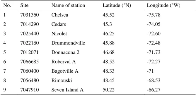
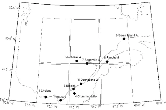
2. Study area and data 183

Observed daily precipitations from nine Environment Canada weather stations located in

184

the province of Quebec (Canada) are used in this study (see Figure 1). The list of stations

185

is presented in Table 1. Predictor variables are obtained from the reanalysis product

186

NCEP/NCAR interpolated on the CGCM3 Gaussian grid (3.75 ° latitude and longitude).

187

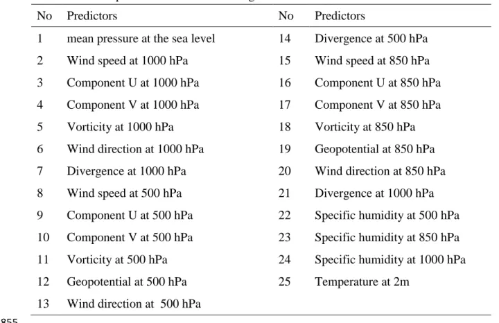
Six grids covering the predictand stations area are selected (see Figure 1), and 25 NCEP

188

predictors are available for each grid (see Table 2). Thus, a total of 150 daily predictors

189

are available for the downscaling process. To reduce the number of predictors, a principal

190

component analysis (PCA) is performed. The first principal components that preserve

191

more than 97% of the total variance are selected. The data sets cover the period

192

between January, 1st 1961 and December, 31st 2000. This record period is divided into

193

two periods for the calibration (1961-1980) and the validation (1981-2000).

194

3. Methodology 195

In this section, the proposed VGLM-NB model is presented. The corresponding

196

probabilistic framework is presented with a description of the conditional

Bernoulli-197

Generalized Pareto regression model and the proposed nonparametric bootstrapping

198

technique.

199

10 3.1. Vector generalized linear model

201

The precipitation amount distribution, at a daily time scale, tends to be strongly skewed,

202

and is commonly assumed to be gamma distributed (Stephenson et al. 1999, Giorgi et al.

203

2001, Yang et al. 2005). In a regression perspective, the generalized linear model (GLM)

204

extends classical regression to handle the normality assumption of the model output. Here

205

the output may follow a range of distributions that allow the variance to depend on the

206

mean such us the exponential distribution family and particularly the Gamma distribution

207

(Coe and Stern 1982, Stern and Coe 1984, Chandler and Wheater 2002). Nevertheless,

208

recent findings suggest that the gamma distribution can be unsuitable for modeling

209

precipitation extremes since it is very restrictive and cannot account for features like

210

heavy tails. Therefore, to treat this issue, other options have been proposed in the

211

literature, particularly the generalized Pareto (GP) and the reverse Weibull (WEI)

212

distributions (Ashkar and Ouarda 1996, Serinaldi and Kilsby 2014). However, due to the

213

fact that the variance does not depend on the mean, these two distributions cannot be used

214

in a GLM. Vector generalized linear models (VGLMs) have been developed to handle

215

this inadequacy (Yee and Stephenson 2007). Instead of the conditional mean only,

216

VGLM provides the entire response distribution by employing a linear regression model

217

where the outputs are vectors of parameters of the selected conditional distribution

218

(Kleiber et al. 2012). Moreover, in downscaling applications, VGLM has a particular

219

advantage since it allows reproducing a realistic temporal variability of the downscaled

220

results by drawing values from the obtained conditional distribution at each forecast step.

221

The structure of the proposed model allows considering a suitable distribution for each

222

station. Among several options proposed in the literature, Gamma, mixed exponential,

11

GP and reverse WEI are the most commonly used and are therefore considered in the

224

current work to represent the precipitation amount on wet days (days with positive values

225

of precipitation amounts, when precipitation falls). However, for the sake of simplicity,

226

only one distribution that provides a good overall fit for all stations is selected. In our

227

study, the examination of the Q-Q plots presented in Figure 2 reveals that all these

228

distributions fit fairly well the precipitation amounts. However, the GP distribution is

229

chosen since it is more successful in reproducing the upper tails. The expression of the

230

zero adjusted GP distribution is given by:

231 232 1 ( ) 1 1 y ; 0 f y y         _{ }    (1) 233 234

where y is the precipitation amount,  ( 0)and  (where1 y 0) are

235

respectively the scale and the shape parameters of the zero-adjusted GP model.

236

Therefore, a mixed Bernoulli–GP distribution with a vector of parameters p( , , )   is

237

considered to represent the whole precipitation distribution that includes both occurrences

238

and amounts in a single distribution. The vector of parameters includes the probability of

239

precipitation



and shape  (where1

 

parameters of the zero adjusted GP distribution. Hence, the proposed precipitation model

242

can be considered as a mixture of Dirac mass on zero (representing the probability on

12

zero) and GP distribution for precipitation amounts (representing positive values of

244

precipitation amounts). Using the VGLM, these parameters are considered to vary for a

245

given day t according to the value of large-scale atmospheric predictors x t( ). However,

246

only the shape parameter  is fixed to guarantee the convergence of the maximum

247

likelihood estimates. For the parameter of the probability of precipitation occurrences we

248

adopt a logistic regression which is expressed as:

249 1 ( ) 1 exp T ( ) t a x t      _ _ (2) 250

where a is the coefficient of the logistic model. The scale parameters ( )t are modeled

251

using an exponential link written as:

252

( )t exp b x tT ( )

  _ _ (3)

253

where bis the coefficient of the model. Thus, the conditional Bernoulli-GP density

254

function for the precipitation y t( ) on a day

t

255 1 1 1 if ( ) = 0 1 exp ( ) [ ( ) | ( )] 1 ( ) 1 1 if ( ) > 0 1 exp ( ) exp ( ) T t T T y t a x t f y t x t y t y t a x t b x t     _  _{  }      _{   }  _{     }  _{       }       _ _  256 (4) 257

The coefficientsa, b and  are obtained following the method of maximum likelihood

258

by minimizing the negative log predictive density (NLPD) cost function (Haylock et al.

259

2006, Cawley et al. 2007, Cannon 2008):

13











L

via the simplex search method of Lagarias et al. (1999). This is a direct search method

262

that does not use numerical or analytic gradients.

263

Now, consider a calibration period of length T and precipitation series at several sites

264

1, 2, ,

j



m

265

very general and can also be conducted using large number of sites.The proposed VGLM

266

regression can be trained separately for each precipitation variablesy_jat the site j, and

267

thus to obtain the estimated parameters ˆ ( )p t and the conditional distributions _j

268

ˆ ( | ( ))_{tj j}

f y x t for each dayt1, 2, ,T. Figure 3a shows the steps involved for estimating

269

the parameters of the VGLM models.

270

3.2. Non parametric bootstrapping technique 271

These dynamic marginal distributions obtained from the VGLM models can be coupled

272

with a random field with uniform margins. Thus, in simulation, generation of the

multi-273

site replicates of the precipitation field is readily achieved by generating properly

274

associated multivariate variants between 0 and 1 with uniform margins, which are

back-275

transformed to synthetic field predictands by applying the inverse cumulative distribution

276

function. To address this point, hidden multivariate variants u t( )=





uniformly distributed between 0 and 1 are extracted where u t_j( ) for j1, ,m are

278

obtained from the following equation:

14 ˆ ( ) ( ( )) j tj j u t F y t (6) 280

where ˆF is the cumulative distribution function at time _tj

t

281

VGLM model. Figure 3b shows the steps involved in obtaining the hidden multivariate

282

variants over the calibration period. First, the VGLM can be evaluated during the

283

calibration period separately for each station. This will allow obtaining the entire

284

conditional distribution for each day from the calibration period. Then the obtained

285

conditional CDFs can be applied to their corresponding predictand values to express

286

precipitation as a probability of non-exceedances ranging from 0 to 1. In order to map

287

( )

j

u t onto the full range of the uniform distribution between 0 and 1, the cumulative

288

probabilities F y t_tj( _j( )) are randomly drawn from a uniform distribution on [0,1( )t ]

289

for dry days. The resulting data matrix u t( )represents values between 0 and 1 that

290

contain the unexplained information by the VGLM model including spatial dependence

291

structures and long term and short term temporal structures.

292

The question that should be addressed in this step is: "how to extract information about

293

the data dependence structure from the data matrixu t( ), and how to preserve this

294

information in the simulation step?”. This information is contained in the ranks matrix R

295

of the data matrix ( )u t (Oakes 1982, Genest and Plante 2003, Song and Singh 2010).

296

Hence, if the ranks of the data matrix u t( )are preserved in the simulation, the data

297

dependence structure will be preserved as well. Recall that copula functions allow

298

modelling the data ranks in order to model the data dependence structure. Thus, the rank

299

matrix R can be modeled using a multivariate copula. In the case of precipitation

15

simulation it would be useful to simulate from a flexible multivariate copula model that

301

preserves both temporal and spatial dependence structures. However achieving such

302

flexibility may require an increasing number of parameters which would makes the

303

copula model less parsimonious and increases the associated uncertainty without ensuring

304

that the ranks of the data will be preserved. In this respect, to avoid any model

305

misspecification, the rank matrix R can be used in the simulation to preserve a great

306

amount of information about the data dependence structure. The idea consists in

307

generating multivariate random variables from the uniform distribution with the same

308

dimension as the matrix R, and then ordering each column according to the

309

corresponding column in R.

310

Finally the synthetic precipitation series during the validation period can be obtained

311

from the VGLM-NB model using the following three steps.

312

(i) Randomly generate multivariate random variables from the uniform

313

distribution with same dimension as the matrix

R

314

period.

315

(ii) Sort each column of the obtained matrix in step (i) according to the

316

corresponding column in R.

317

(iii) Apply the inverse cumulative Bernoulli-GP distribution expressed in Equation

318

(3) for each site j and for each forecast day t from the validation period to the

319

sorted matrix obtained in step (ii).

16

Let us now consider the univariate variant u tj( ) at a site j and the same variant 321

( )

j

u th lagged by h days. Since the rank column R_j on this site j is preserved, the

322

ranks matrix R of the data matrix h_j [u t u t_j( ), _j( h)] will be preserved as well. This

323

implies that the proposed approaches can be expected to preserve the temporal correlation

324

at individual sites during the simulation. The proposed NB approach is similar to a

325

copula, since both are based on the generation of uniformly distribution random variables

326

that are correlated, except that copula allows modelling the ranks matrix whereas the

327

proposed approach mimics the data ranks rather than modeling them.

328

As discussed by Serinaldi and Kilsby (2014), taking into account the spatial correlation

329

and the short term autocorrelation in a probabilistic regression model can be introduced

330

in two ways: (i) by introducing the precipitation at previous time steps as an additional

331

covariate, or (ii) by using a random field with uniform marginals and a suitable

spatio-332

temporal structure. The first way implies a sequential simulation; it can be used for cases

333

involving a small number of sites (Serinaldi 2009, Kleiber et al. 2012). In the second

334

way, multisite characteristics and temporal autocorrelation are introduced in the

335

simulation stage using correlated random numbers with uniform marginal distributions.

336

This second way is adopted in the current work. This technique avoids a sequential

337

simulation conditioned on the simulation of the precipitation at the previous time steps

338

and can be adapted for a large number of sites. In the proposed approach the probabilistic

339

regression component uses a single discrete-continuous distribution and thus avoids the

340

split between occurrence process (the transition between wet and dry days) and

341

precipitation amount process (positive precipitation values in wet days). In this way, the

342

number of the random field substrates to be used in the simulation stage is reduced from

17

two (one for the occurrence process and one for the amount process) to one, thus making

344

the model more parsimonious.

345

3.3. Quality assessment of downscaled precipitation 346

To assess the performance of the proposed NB model, we compare it to

VGLM-347

MAR which is a downscaling model using the same mixed Bernoulli-Generalized Pareto

348

distribution and extended to multisite tasks using a first order multivariate autoregressive

349

random field framework (Ben Alaya et al. 2015).

350

3.3.1. Quality assessment of univariate characteristics 351

Two approaches are considered for the quality assessment of univariate characteristics of

352

the VGLM-NB model. The first approach is based on a direct comparison between the

353

estimated and observed values using statistical criteria, while the second approach is

354

based on calculating climate indices. In the two validation approaches, the VGLM-NB

355

model results are compared to those obtained using the VGLM-MAR.

356

In the first validation approach, four statistical criteria are used for model validation.

357

These criteria are:

358













18 a FAR b  (10) 362

where n denotes the number of observations,

t

obs

y refers to the observed value,

t

est y is

363

the estimated value, t denotes the day,  is the standard deviation, a the number of

364

false alerts for observed dry days, and b is the total number of observed dry days. 365

The first criterion is the mean error (ME) which is a measure of accuracy. The second

366

criterion is the root mean square error (RMSE) which is given by an inverse measure of

367

the accuracy and must be minimized, and the third criterion D measures the difference

368

between observed and modeled variances, this criterion evaluates the performance of the

369

model in reproducing the observed variability. The last criterion, the false alarm rate

370

(FAR), is the fraction of false alerts associated with observed dry days and must be

371

minimized.

372

In a second validation approach, a set of several precipitation indices that reflect

373

precipitation variability on a seasonal and monthly basis are considered. Five indices

374

related to precipitation amounts are considered: the mean precipitation of wet days

375

(MPWD), the 90th percentile of daily precipitation (Pmax90), the maximum 1-day

376

precipitation (PX1D), the maximum 3-day precipitation (PX3D), and the maximum 5-day

377

precipitation (PX5D). In addition, three other indices are considered for precipitation

378

occurrences: the maximum number of consecutive wet days (WRUN), the maximum

379

number of consecutive dry days (DRUN) and the number of wet days (NWD). All

380

indices are calculated on a monthly time scale, whereas the P90max is calculated on a

381

seasonal time scale.

19

3.3.2. Quality assessment of multisite characteristics 383

Multisite characteristics are verified using scatter plots of observed and modeled lag-0

384

and lag-1 cross-correlations and log odds ratios (LOR). Lag-0 cross correlations

385

correspond to cross correlations between all pairs of data (not lagged in time) whereas

386

Lag-1 cross correlations correspond to cross correlations between all pairs of data lagged

387

by 1 day.

388

A log-odds ratio between a pair of stations i and j is expressed as:

389 , , , , , 00 11 ln 10 01 i j i j i j i j i j p p LOR p p         , (11) 390

Where p00 , 11 , 10 , 01_{i j,} p _{i j,} p _{i j,} p _{i j,} are the joint probabilities of no rain at either one of the

391

two stations, rain at both stations, rain at station i and no rain at station j, and finally no

392

rain at station i and rain at station j, respectively. The log odds ratio provides a measure

393

of the spatial correlation between precipitation occurrences at each pair of stations where

394

higher values indicate better defined spatial dependence (Mehrotra et al. 2004, Mehrotra

395

and Sharma 2006).

396

The dynamics of flood events are strongly related to the simultaneous occurrence of

397

extreme precipitation at several sites. A pairwise correlation is often used for the

398

specification of multisite precipitation models (this is the case of the VGLM-MAR). On

399

the other hand multisite properties of extreme precipitation could be related to

higher-400

order correlations than a traditional pairwise correlation (Serinaldi et al. 2014). In this

401

respect, a diagnostic based on higher order correlations between extreme precipitations is

402

necessary but often ignored. To this end, Bárdossy and Pegram (2009) introduced the

20

binary entropy as a measure of dependence in a given triplet. This measure overcomes a

404

pairwise validation in order to look effectively at the high-order dependence properties.

405

The entropy theory was first formulated by (Shannon 1948) to provide a measure of

406

information contained in a set of data. To calculate the binary entropy, we first fix a given

407

quantile threshold to divide each precipitation series into binary sets by allocating 0 to the

408

lower partition defined by the threshold and 1 otherwise. At each day, the eight possible

409

states of a given binary triple can be defined using the set





410

the eight binary probabilitiesp i j k( , , ), for i j k, , 0,1 can be calculated over all days

411

from the validation period. For example, p(1,1,1) represents the probability that all three

412

binary sets on a given day are simultaneously equal to 1, and p(0, 0, 0) that they are all

413

equal to 0. The binary entropy H can be computed as

414 1 , , 0 ( , , ) ln( ( , , )). i j k H p i j k p i j k   



Hence, the lower the entropy is, the stronger will be the association between the variables

416

at a given threshold.

417

4. Results 418

The VGLM-NB model was trained for the calibration period (1960-1980), using

419

precipitation data series from the nine stations and the 40 predictors obtained by the PCA.

420

Once the parameters of the conditional Bernoulli-GA distribution (_j( ),t _j( )t and_j( )t )

421

have been estimated for each day

t

422

obtained conditional marginal distributions were used to obtain the hidden variables

u t

( )

21

and then to calculate the rank data matrix R. Finally, for each of the nine sites, 1000 daily

424

precipitations series were generated during the validation period (1981-2000) using

425

VGLM-NB described in Section 3 and the VGLM-MAR for comparisons. We assume

426

that 1000 simulations are sufficiently enough to provide stable estimates of precipitation

427

characteristics. Figure 4 shows an example of one precipitation simulation obtained using

428

the VGLM-NB model at Cedars station during the year 1981. Based on the simulated

429

series, VGLM-NB seems to be able to preserve at site properties of the natural process of

430

both precipitation amounts and precipitation occurrences.

431

For the evaluation of the univariate characteristics of VGLM-NB and VGLM-MAR using

432

statistical criteria, the RMSE and ME where calculated using the conditional means of

433

1000 realisations, whereas the differences between observed and modeled variances

434

where calculated using the mean variance values of the 1000 simulations. Table 3 shows

435

values of the obtained criteria. Generally, the two compared models give similar results

436

in terms of RMSE, ME and D. This result is expected since both NB and

VGLM-437

MAR have the same probabilistic regression component. For precipitation occurrences, in

438

terms of FAR results show that VGLM-NB has fewer FAR over all stations. This result

439

shows that, although both VGLM-NB and VGLM-MAR are trained using the same

440

probabilistic regression component (the Bernoulli-generalized Pareto regression model),

441

the non-parametric bootstrapping technique leads to better at-site results than the MAR

442

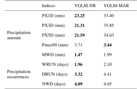
approach. In addition, by the evaluation of univariate characteristics using precipitation

443

indices, the RMSE values of these indices (presented in Table 4) show that VGLM-NB

444

performs better than VGLM-MAR for all indices, except for the 90th percentile of daily

445

precipitation. This result demonstrates that the VGLM-NB is more able to represent

22

precipitation variability on a monthly basis than the VGLM-MAR. To evaluate the ability

447

of both VGLM-NB and VGLM-MAR to simulate short term autocorrelation, Figure 5

448

shows observed and modeled lag-1 autocorrelation for precipitation series at the nine

449

stations during the validation period. It can be seen from Figure 5 that VGLM-NB

450

preserves more adequately the lag-1 autocorrelation at a single site.

451

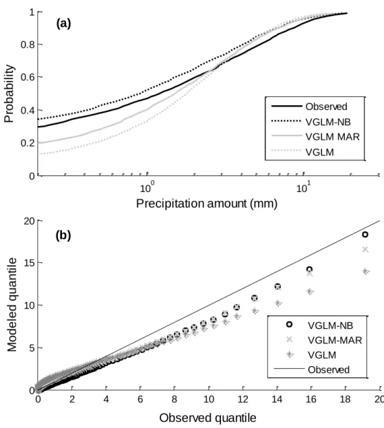
To evaluate the ability of the models to simulate spatially realistic precipitation fields,

452

Figure 6 compares the distribution of observed and downscaled daily average

453

precipitations over the 9 stations for VGLM-NB, VGLM-MAR and univariate VGLM

454

without multisite extension. The comparison with the univariate VGLM is beneficial to

455

identify the real gain contributed by the two multisite components of VGLM-NB and

456

VGLM-MAR. The observed and modeled CDFs are presented in Figure 6.a and the Q-Q

457

plots for quantiles corresponding to non-exceeded probabilities ranging between 0.01 and

458

0.99 with a step of 0.01 in Figure 6.b. Results indicate that the performance of

VGLM-459

NB in reproducing the distribution of daily average precipitation is satisfactory compared

460

to VGLM and VGLM-MAR. Both VGLM and VGLM-MAR underestimate the higher

461

precipitation amounts and overestimates the lower precipitation amounts. Although

462

VGLM-NB slightly overestimates observed quantiles, it tends to fairly well reproduce

463

low and high values. This overestimation may be explained by the fact that VGLM-NB

464

supposes that the rank matrix of the variants u t( ) remain the same during the validation

465

period.

466

Figure 7 shows scatterplots between observed and modeled lag-0 and lag-1

cross-467

correlations for all station pairs considering only wet days during the validation period.

468

Lag-0 cross-correlation is presented in Figure 7.a and lag-1 cross-correlation in Figure

23

7.b. The correlation values for each model are obtained using the mean of the correlation

470

values calculated from the 1000 realisations. For lag-0 cross-correlation, the points

471

correspond to all 36 combinations of pairs of stations, while for lag-1 cross-correlation

472

points correspond to all 81 combinations because lag-1 cross-correlations are generally

473

not symmetric. Figure 7.a shows that observed values of lag-0 cross-correlation range

474

between -0.02 and 0.65. VGLM-NB gives better preservation of lag-0 cross-correlation

475

than both VGLM-MAR and traditional VGLM. Because VGLM is not a multisite model,

476

it gives the poorest performances and generally underestimates lag-0 cross-correlations.

477

Figure 5b indicates that, for the lag1 crosscorrelation, observed values range between

-478

0.1 and 0.28. For VGLM-NB the performance in reproducing lag-1 cross correlation is

479

less good than the on corresponding to lag-0 cross correlation. However, this

480

performance seems to be always better than the two other models.

481

To further evaluate the multisite performance, Figure 8.a presents observed and modeled

482

log odds ratios for the VGLM-NB, VGLM-MAR and univariate VGLM at all stations.

483

Results indicate that the VGLM-NB model provides very close correspondence with

484

observed log odds ratios and gives better results than the two other models. VGLM-MAR

485

outperforms the univariate VGLM but its results are less accurate than VGLM-NB,

486

especially when the observed correlations are high.

487

Figure 9 shows scatter plots of observed and modeled binary entropy for precipitation

488

occurrences (Figure 9a) and at three quantile thresholds: 0.75 (Figure 9.b), 0.90 (Figure

489

9.c) and 0.975 (Figure 9.d). Points correspond to all combinations of stations triplets. It

490

can be seen from Figure 9.a that simulated precipitation occurrences using both VGLM

491

and VGLM-MAR data exhibit higher binary entropy values than observed data. Similar

24

results were found for binary entropy corresponding to the quantile thresholds 0.75, 0.90

493

and 0.95. This result indicates that the Gaussian dependence structure is not enough to

494

capture the stronger association of extreme precipitation. It is clear that the VGLM-NB is

495

closer to the data across the range of the binary entropy H than the VGLM-MAR model,

496

indicating that non-parametric bootstrapping simulation is an improvement over the

497

multivariate autoregressive Gaussian framework. In reality, this result is expected, since

498

the VGLM-MAR captures the spatial structure by modeling a combination of bivariate

499

relationships using the Gaussian copula. Improving the capture of spatial structure using

500

parametric models requires the application of high-dimensional copulas such us a vine

501

copula.

502

5. Discussions 503

Unlike the VGLM-MAR, an attractive characteristic of the proposed VGLM-NB is that

504

pairwise correlations are not used for the model definition. Indeed, the employed

non-505

parametric bootstrapping technique does not model dependency structures but mimics the

506

observed data ranks to preserve the unexplained multisite properties by the VGLM. As it

507

is the case for most resampling methods (Ouarda et al. 1997, Buishand and Brandsma

508

1999, Buishand and Brandsma 2001, Mehrotra and Sharma 2009, Lee et al. 2012), this

509

approach is data driven, non-parametric and thus avoiding any model misspecification

510

when preserving multisite properties. However, while resampling models suffer from the

511

inability to generate values that are more extreme than those observed, the probabilistic

512

regression component of the proposed hybrid model allows overcoming this drawback.

513

Indeed, regression methods and resampling techniques can be combined to take

514

advantage of their strengths for downscaling tasks. For this purpose, a widely used

25

approach consists in using resampling or randomisation methods to address the inability

516

of the traditional regression component to preserve the temporal variability and multisite

517

properties (Jeong et al. 2012, Jeong et al. 2013, Khalili et al. 2013). These hybrid

518

approaches are based on a static noise observed during the calibration of the regression

519

component. Therefore, the part of the variability which is explained by the randomization

520

component does not depend on the predictors, and thus, it is supposed to be constant in a

521

changing climate. For this reason, this traditional hybrid structure may not represent local

522

change in the temporal variability in a climate change simulation. Hence, the hybrid

523

structure employed here to describe the VGLM-NB (as well as the VGLM-MAR), allows

524

the temporal variability to be reproduced in the regression component (using the VGLM

525

component) and thus it may change in the future according to the large scale atmospheric

526

predictors.

527

Although the proposed non parametric approach allows preserving the multisite

528

dependence structure at gauged sites, this dependence structure is still unknown. In

529

regionalization applications where simulations at ungaged locations are required it is

530

imperative to know the structure of the spatial dependence. In such a situation, a spatial

531

model is required and thus modelling the data ranks through copulas would be more

532

advantageous. Another limitation of the proposed approach is that the data rank matrix of

533

the hidden variants u t( ) is supposed to be the same (i.e. stationary) in the future. In this

534

respect, allowing the dependence to be dynamic requires also a parametric modelling.

535

It should be mentioned that a very important point that has not been considered in this

536

work is the selection of predictor variables. The selection of predictor variables in the

537

development of statistical downscaling models requires comprehensive considerations. In

26

the case of precipitation, the best description of the conditional distribution may require

539

the use of different subsets of predictor variables for precipitation amounts and

540

precipitation occurrences. Predictor variables must be physically sensible, realistically

541

modeled by the AOGCM, and able to fully reflect the climate change signal. In the

542

current work, NCEP/NCAR data are used for calibration and validation in order to assess

543

the potential of the proposed approach, although the final objective is to use AOGCM

544

outputs. Even if NCEP data are complete and physically consistent they are still subject

545

to model biases (Hofer et al. 2012). NCEP variables which are not assimilated (such as

546

precipitation), but generated by the parameterizations based on dynamical model can

547

significantly deviate from real weather. The use of such variables for the calibration and

548

validation of empirical downscaling techniques may not be a good idea, since it may

549

induce a significant deviation of the modeled relationships predictors/predictands from

550

the reality which makes evaluation of downscaling techniques more difficult.

551

The downscaling problem as is tackled in this paper can be viewed as a regression

552

problem, where we try to predict climate variables at small scale from climate variables

553

at synoptic scale. However, due to the large literature that addresses the precipitation

554

modelling in general, the downscaling issue may be viewed as an adjustment of existed

555

precipitation models to account for large scale climate drivers (GCM precipitation, SLP,

556

wind speed, etc.). Wilks (2010) suggested that these adjustments can be accomplished in

557

two ways: (i) through imposed changes in the corresponding monthly statistics, (ii) or by

558

controlling the precipitation model parameters by daily variations in simulated

559

atmospheric circulation. In this context, the VGLM component of the proposed model

560

focuses on the second way in the adjustment procedure. Indeed, through the VGLM

27

component, large scale climate drivers are employed as exogenous variables to describe

562

parameters of the mixed Bernoulli-GP distribution.

563

6. Conclusions 564

A VGLM-NB model is proposed in this paper for simultaneously downscaling AOGCM

565

predictors to daily multisite precipitation. The VGLM-NB relies on a probabilistic

566

modeling framework in order to predict the conditional Bernoulli-Generalized Pareto

567

distribution of precipitation at a daily time scale. A non-parametric bootstrapping

568

technique is proposed to preserve a realistic representation of relationships between sites

569

at both time and space. This rank-based sampling method is easy to implement and does

570

not model the dependency structures, but mimic the observed historical characteristics of

571

multisite precipitation and thus avoids any model specification error. However, it should

572

be mentioned that it cannot be used for simulations at ungagged locations. Indeed, in such

573

a situation, modeling the data ranks through spatial copulas would be more appropriate.

574

The developed model was then applied to generate daily precipitation series at nine

575

stations located in the southern part of the province of Quebec (Canada). Model

576

evaluations suggest that the VGLM-NB model is capable of generating series with

577

realistic spatial and temporal variability. The developed model can be easily applied to

578

other variables such as temperature and wind speed making it a valuable tool not only for

579

downscaling purposes but also for environmental and climatic modelling, where often

580

non-normally distributed random variables are involved.

581

28 7. References

583

AghaKouchak, A. (2014). "Entropy–copula in hydrology and climatology." Journal of 584

Hydrometeorology 15(6): 2176-2189. 585

586

AghaKouchak, A., A. Bárdossy and E. Habib (2010). "Conditional simulation of remotely sensed 587

rainfall data using a non-Gaussian v-transformed copula." Advances in Water Resources 33(6): 588

624-634. 589

590

Ashkar, F. and T. B. Ouarda (1996). "On some methods of fitting the generalized Pareto 591

distribution." Journal of Hydrology 177(1): 117-141. 592

593

Bárdossy, A. (2006). "Copula-based geostatistical models for groundwater quality parameters." 594

Water Resour. Res. 42(11): W11416. 595

596

Bárdossy, A. and J. Li (2008). "Geostatistical interpolation using copulas." Water Resour. Res. 597

44(7): W07412.

598 599

Bárdossy, A. and G. G. S. Pegram (2009). "Copula based multisite model for daily precipitation 600

simulation." Hydrology and Earth System Sciences 13(12): 2299-2314. 601

602

Bargaoui, Z. K. and A. Bárdossy (2015). "Modeling short duration extreme precipitation patterns 603

using copula and generalized maximum pseudo-likelihood estimation with censoring." Advances 604

in Water Resources 84: 1-13. 605

606

Ben Alaya, M. A., F. Chebana and T. Ouarda (2014). "Probabilistic Gaussian Copula Regression 607

Model for Multisite and Multivariable Downscaling." Journal of Climate 27(9). 608

609

Ben Alaya, M. A., F. Chebana and T. B. Ouarda (2015). "Probabilistic Multisite Statistical 610

Downscaling for Daily Precipitation Using a Bernoulli–Generalized Pareto Multivariate 611

Autoregressive Model." Journal of Climate 28(6): 2349-2364. 612

613

Benestad, R. E., I. Hanssen-Bauer and D. Chen (2008). Empirical-statistical downscaling, World 614

Scientific. 615

616

Bremnes, J. B. (2004). "Probabilistic forecasts of precipitation in terms of quantiles using NWP 617

model output." Monthly Weather Review 132(1). 618

29

Buishand, T. A. and T. Brandsma (1999). "Dependence of precipitation on temperature at 620

Florence and Livorno (Italy)." Climate Research 12(1): 53-63. 621

622

Buishand, T. A. and T. Brandsma (2001). "Multisite simulation of daily precipitation and 623

temperature in the Rhine basin by nearest‐neighbor resampling." Water Resources Research 624

37(11): 2761-2776.

625 626

Cannon, A. J. (2008). "Probabilistic multisite precipitation downscaling by an expanded 627

Bernoulli-gamma density network." Journal of Hydrometeorology 9(6): 1284-1300. 628

629

Cannon, A. J. (2011). "Quantile regression neural networks: Implementation in R and application 630

to precipitation downscaling." Computers & Geosciences 37(9): 1277-1284. 631

632

Cawley, G. C., G. J. Janacek, M. R. Haylock and S. R. Dorling (2007). "Predictive uncertainty in 633

environmental modelling." Neural Networks 20(4): 537-549. 634

635

Chandler, R. E. and H. S. Wheater (2002). "Analysis of rainfall variability using generalized linear 636

models: a case study from the west of Ireland." Water Resources Research 38(10): 10-11-10-11. 637

638

Chebana, F. and T. B. Ouarda (2011). "Multivariate quantiles in hydrological frequency analysis." 639

Environmetrics 22(1): 63-78. 640

641

Coe, R. and R. Stern (1982). "Fitting models to daily rainfall data." Journal of Applied 642

Meteorology 21(7): 1024-1031. 643

644

Conway, D., R. Wilby and P. Jones (1996). "Precipitation and air flow indices over the British 645

Isles." Climate Research 7: 169-183. 646

647

Czado, C., E. C. Brechmann and L. Gruber (2013). Selection of vine copulas. Copulae in 648

Mathematical and Quantitative Finance, Springer: 17-37. 649

650

El Adlouni, S., B. Bobée and T. Ouarda (2008). "On the tails of extreme event distributions in 651

hydrology." Journal of Hydrology 355(1): 16-33. 652

653

Eum, H.-I., P. Gachon, R. Laprise and T. Ouarda (2012). "Evaluation of regional climate model 654

simulations versus gridded observed and regional reanalysis products using a combined 655

weighting scheme." Climate Dynamics 38(7-8): 1433-1457. 656

30

Fang, H.-B., K.-T. Fang and S. Kotz (2002). "The meta-elliptical distributions with given 658

marginals." Journal of Multivariate Analysis 82(1): 1-16. 659

660

Fasbender, D. and T. B. M. J. Ouarda (2010). "Spatial Bayesian Model for Statistical Downscaling 661

of AOGCM to Minimum and Maximum Daily Temperatures." Journal of Climate 23(19): 5222-662

5242. 663

664

Friederichs, P. and A. Hense (2007). "Statistical downscaling of extreme precipitation events 665

using censored quantile regression." Monthly Weather Review 135(6). 666

667

Genest, C. and F. Chebana (2015). "Copula modeling in hydrologic frequency analysis." In 668

Handbook of Applied Hydrology (V.P. Singh, Editor) McGraw-Hill, New York, (in press). 669

670

Genest, C. and J. F. Plante (2003). "On Blest's measure of rank correlation." Canadian Journal of 671

Statistics 31(1): 35-52. 672

673

Giorgi, F., J. Christensen, M. Hulme, H. Von Storch, P. Whetton, R. Jones, L. Mearns, C. Fu, R. 674

Arritt and B. Bates (2001). "Regional climate information-evaluation and projections." Climate 675

Change 2001: The Scientific Basis. Contribution of Working Group to the Third Assessment 676

Report of the Intergouvernmental Panel on Climate Change [Houghton, JT et al.(eds)]. 677

Cambridge University Press, Cambridge, United Kongdom and New York, US. 678

679

Gräler, B. (2014). "Modelling skewed spatial random fields through the spatial vine copula." 680

Spatial Statistics 10: 87-102. 681

682

Guerfi, N., A. A. Assani, M. Mesfioui and C. Kinnard (2015). "Comparison of the temporal 683

variability of winter daily extreme temperatures and precipitations in southern Quebec (Canada) 684

using the Lombard and copula methods." International Journal of Climatology. 685

686

Harpham, C. and R. L. Wilby (2005). "Multi-site downscaling of heavy daily precipitation 687

occurrence and amounts." Journal of Hydrology 312(1): 235-255. 688

689

Haylock, M. R., G. C. Cawley, C. Harpham, R. L. Wilby and C. M. Goodess (2006). "Downscaling 690

heavy precipitation over the United Kingdom: A comparison of dynamical and statistical 691

methods and their future scenarios." International Journal of Climatology 26(10): 1397-1415. 692

693

Hessami, M., P. Gachon, T. B. M. J. Ouarda and A. St-Hilaire (2008). "Automated regression-694

based statistical downscaling tool." Environmental Modelling & Software 23(6): 813-834. 695

31

Hobæk Haff, I., A. Frigessi and D. Maraun (2015). "How well do regional climate models simulate 697

the spatial dependence of precipitation? An application of pair‐copula constructions." Journal of 698

Geophysical Research: Atmospheres 120(7): 2624-2646. 699

700

Hofer, M., B. Marzeion and T. Mölg (2012). "Comparing the skill of different reanalyses and their 701

ensembles as predictors for daily air temperature on a glaciated mountain (Peru)." Climate 702

Dynamics 39(7-8): 1969-1980. 703

704

Jeong, D., A. St-Hilaire, T. Ouarda and P. Gachon (2012). "Comparison of transfer functions in 705

statistical downscaling models for daily temperature and precipitation over Canada." Stochastic 706

Environmental Research and Risk Assessment 26(5): 633-653. 707

708

Jeong, D., A. St-Hilaire, T. Ouarda and P. Gachon (2013). "A multivariate multi-site statistical 709

downscaling model for daily maximum and minimum temperatures." Climate Research 54(2): 710

129-148. 711

712

Jeong, D. I., A. St-Hilaire, T. B. M. J. Ouarda and P. Gachon (2012). "Multisite statistical 713

downscaling model for daily precipitation combined by multivariate multiple linear regression 714

and stochastic weather generator." Climatic Change 114(3-4): 567-591. 715

716

Joe, H. (1997). Multivariate models and multivariate dependence concepts, CRC Press. 717

718

Khalili, M., V. T. Van Nguyen and P. Gachon (2013). "A statistical approach to multi‐site 719

multivariate downscaling of daily extreme temperature series." International Journal of 720

Climatology 33(1): 15-32. 721

722

Kleiber, W., R. W. Katz and B. Rajagopalan (2012). "Daily spatiotemporal precipitation simulation 723

using latent and transformed Gaussian processes." Water Resources Research 48(1). 724

725

Lagarias, J. C., J. A. Reeds, M. H. Wright and P. E. Wright (1999). "Convergence properties of the 726

Nelder-Mead simplex method in low dimensions." SIAM Journal on Optimization 9(1): 112-147. 727

728

Lee, T., R. Modarres and T. Ouarda (2013). "Data‐based analysis of bivariate copula tail 729

dependence for drought duration and severity." Hydrological Processes 27(10): 1454-1463. 730

731

Lee, T., T. B. Ouarda and C. Jeong (2012). "Nonparametric multivariate weather generator and 732

an extreme value theory for bandwidth selection." Journal of Hydrology 452: 161-171. 733