The dynamics of sustained reentry in a loop model with discrete gap junction resistance

AVIS

Ce document a été numérisé par la Division de la gestion des documents et des archives de l’Université de Montréal.

L’auteur a autorisé l’Université de Montréal à reproduire et diffuser, en totalité ou en partie, par quelque moyen que ce soit et sur quelque support que ce soit, et exclusivement à des fins non lucratives d’enseignement et de recherche, des copies de ce mémoire ou de cette thèse.

L’auteur et les coauteurs le cas échéant conservent la propriété du droit d’auteur et des droits moraux qui protègent ce document. Ni la thèse ou le mémoire, ni des extraits substantiels de ce document, ne doivent être imprimés ou autrement reproduits sans l’autorisation de l’auteur.

Afin de se conformer à la Loi canadienne sur la protection des renseignements personnels, quelques formulaires secondaires, coordonnées ou signatures intégrées au texte ont pu être enlevés de ce document. Bien que cela ait pu affecter la pagination, il n’y a aucun contenu manquant.

NOTICE

This document was digitized by the Records Management & Archives Division of Université de Montréal.

The author of this thesis or dissertation has granted a nonexclusive license allowing Université de Montréal to reproduce and publish the document, in part or in whole, and in any format, solely for noncommercial educational and research purposes.

The author and co-authors if applicable retain copyright ownership and moral rights in this document. Neither the whole thesis or dissertation, nor substantial extracts from it, may be printed or otherwise reproduced without the author’s permission.

In compliance with the Canadian Privacy Act some supporting forms, contact information or signatures may have been removed from the document. While this may affect the document page count, it does not represent any loss of content from the document.

The Dynamics of Sustained Reentry in a Loop Model with Discrete Gap Junction Resistance

Par Wei Chen

Institute de génie biomédical Faculté de médecine

Mémoire présenté

à

la Faculté des études supérieures en vue de l'obtention du grade de Maîtrise ès sciences appliquées

en génie biomédical

Avril 2007

r ' Université de Montréal

. Faculté des études supérieures

Ce mémoire intitulé:

The Dynamics of Sustained Reentry in a Loop Model with Discrete Gap Junction Resistance

présenté par: Wei Chen

a été évalué par un jury composé des personnes suivantes:

A. Robert LeBlanc, Ing., D.Sc.A président-rapporteur

Alain Vinet, Ing., Ph.D. directeur de recherche

Jacques Bélair, Ph.D. membre du jury

Résumé

Lors d'un battement cardiaque normal, l'activation électrique débute dans le nœud sinus al et se propage dans les deux oreillettes. Elle atteint ensuite le faisceau de His, puis finalement les fibres de Purkinje qui distribuent l'excitation dans les ventricules pour déclencher la con-traction. Cette propagation se produit parce que les myocytes cardiaques peuvent produire un potentiel d'action quand ils sont dépolarisés au-delà d'un seuiL que les cellules sont connectées électriquement, la dépolarisation d'une partie du tissu cardiaque provoque une augmentation du potentiel dans le tissu voisin, jusqu'à ce que ce dernier atteigne son seuil d'excitation et devienne à son tour une source qui permet à la propagation de se poursuivre. Les propriétés électriques de la membrane des myocytes cardiaques ventriculaires ont été décrites par différents modèles mathématiques. Dans ce travail, nous utilisons une variante du modèle de Beeler et Reuter, qui fournit une représentation de type Hodgkin-Huxley des conductances de courants ioniques membranaires. En voltage imposé, le modèle est constitué par un système d'équations différentielles ordinaires qui décrivent la dynamique temporelle du potentiel membranaire, des variables portes contrôlant la conductance des différents canaux ioniques et de la concentration interne de calcium. Pour' ce qui est de description du tissu ventriculaire, la plupart des travaux de modélisation considèrent la membrane et les milieux intra et extracellulaires comme continus, de telle sorte que les flux de courants à travers la membrane et les milieux résistifs intra et extracellulaires sont représentés par une équation aux dérivées partielles. Cependant, le tissu cardiaque est constitué par des myocytes discrets, dont les milieux intracellulaires sont joints par des protéines. Ces

agissent comme des résistances connectant électriquement les milieux intracellulaires des cellules voisines. C'est ce dernier point de vue que nous avons adopté dans cet mémoire.

Le but de notre étude est d'examiner l'effet des résistances de jonction sur les car-actéristiques des réent rées pouvant se produire dans un modèle de boucle unidimension-nelle de cellules cardiaques. La réentrée cardiaque correspond à la propagation soutenue

d'un front d'activation autour d'un obstacle anatomique ou fonctionnel. La propagation autour d'une boucle unidimensionnelle est donc le modèle de réentrée le plus simple. Des travaux précédents sur des boucles uniformes et continues, dont les propriétés membranaires étaient représentées par divers modèles ioniques, ont montré que la réent rée pouvait demeurer soutenue mais devenir quasi-périodique quand la dimension de la boucle était inférieure à une longueur critique Lcrit et qu'elle s'interrompait pour des longueurs inférieures à une longueur minimale Lmin. Ces travaux ont montré que la transition de réent rée périodique à

quasi-périodique était contrôlée par les courbes de restitution et de dispersion, décrivant respectivement la variation de la durée des potentiels d'action et de la vitesse de propaga-tion en foncpropaga-tion de la prématurité de la stimulapropaga-tion. Nous avons étudié une boucle formée de cellules discrètes par des résistances de jonction et avons développé une méthode numérique pour solutionner le système de réaction-diffusion décrivant ce milieu. Nous avons trouvé que la diminution de LCl'it et de Lmin résultant de l'augmentation des résistances de jonction n'était pas réductible à un simple facteur d'échelle appliqué sur les résultats des boucles uniformes continues. Nous avons plutôt montré que les résultats étaient expliqués par les changements dans les courbes de restitution et de dispersion induits par l'effet des résistances de jonction sur la dynamique locale.

Mots clé : Potentiel d'action, Réentrée, Réentrée stable périodique et quasi-périodique, Résistance de jonction, Bifurcation, Durée de potentiel d'action, Intervalle diastolique, Longueur de boucle, Temps de conduction, Vitesse de conduction, Mode-O, Mode-l.

Abstract

In a normal heartbeat, electrical activation starts from the SA node and propagates to both atria. It travels successively through the AV node, the His Bundle and finally the Purkinje fibers that distribute the excitation and contract ventricles.

The electrical activation is formed by the unequal ionic distribution on both sides of the sarcoplasmic membrane, producing a difference of potential between the intra and extracel-lular media. The electrical properties of the ventricular cardiac myocytes are described by the different mathematical models. The Hodgkin-Huxley model and Beeler-Reuter model use the ordinary differential equation to simulate membrane potential as a time-dependent function. The bifurcation phenomena of action potential duration and diastolic interva.l are simulated, which are proved by the finite difference model.

The action potential propagates in cardiac tissue. The low-dimensional model was em-ployed. In the one-dimensional model, since cardiac tissue is regarded as the uniform con-tinuous cable, bifurcation phenomena are simulated, and these results are proven by the integral delay model. The other model is that the gap junction resistance exists between cells. The propagation delay is shown between cells. The action potential propagates in the one-dimensional ring with the gap junction resistance, shown to be the most interesting in recent research.

The purpose of our study is to investigate the effect of gap junction resistance on the characteristics of reentry in a one-dimensional ring of model cardiac tissue. Tachyarrhythmia is commonly induced by reentry. Cardiac reentry corresponds to the self-sustained propaga-tion of an activapropaga-tion front around a funcpropaga-tiona.l or anatomica.l obstacle. Propagapropaga-tion around a one-dimensional ring is the simplest model of reentry. Previous work on a uniform contin-uous I-D ring model, with membrane properties represented by an ionic model, has shown that reentry was still sustained but quasiperiodic, below a critical length Lcrit , and that it was blocked for rings shorter than a minimum length Lmin. The transition from periodic to

quasiperiodic reentry was shown to be controlled by the restitution and dispersion curves, giving respectively the action potential duration and speed of propagation as a function of prematurity. However, cardiac myocytes are connected by discrete channels, called gap junctions, acting as resistance between the cells. 'vVe have studied a ring of cells connected by discrete gap resistances (R) and developed a numerical method of solving the resulting reaction-diffusion system. We found that the decrease of Lcrit and Lmin as a function of R

was not a simple scaling of the results of the uniform ring, but could be explained by the change in the restitution and dispersion C"llrves induced by the resistance that modulates the effect of neighbors on the local dynamics.

Keywords: Action potential, Reentry, Stable Reentry, Quasiperiodic reentry, Gap junction resista.nce, Bifurcation, Action potential duration, Diastolic interval, Ring length, Conduc-tion time, ConducConduc-tion velocity, Mode-O, Mode-l.

Contents

Résumé. Abstract List of Tables List of Figures Acknow ledgments 1 Introduction III v lX XU XV 1 1.1 Membrane Potential . . . 1

1.2 Rhythmical Excitation of the Heart 4

1.3 Arrhythmias. 4

1.4 Reentry .. . 5

1.5 Beeler-Reuter-Roberge-Drouard Model of the Cardiac ventricular myocyte 7 1.5.1 Description . . . 7 1.5.2 Dynamics on the Space-Clamped M BR 11 1.6 Modified Beeler-Reuter Loop Model . . . 17 1.7 Role of gap junction in the propagation of the cardiac action potential . 24

2 Dynamics of Sustained Reentry in a Loop Model with Discrete Gap

Junc-tion Resistance 34 2.1 Introduction 2.2 Methods 2.3 Results. 36 37

40

2.4

Lcril., Perit in transition to QP reentry.

2.5

QP reentry

..

.

~ . .

2.5.1

mode-O Q P reentry

2.5.2

Higher Q P Modes

2.6

Discussion and Summary .

3 Discussion and Conclusion

Appendix 1: Methods to Solve the One-Dimensional Cable Equation with Discrete Gap Junction Resistance

1 2 3

Ca1culation of terms A, Band C Solution of

V; . . . .

Connection the Cell .

Appendix II: Agreement of coauthors of article

Bibliography

41

44

45

48

49

52 57 58

60

61

70 71

List of Tables

List of Figures

1.1 Schematic diagram of transmembrane action potential for ventricular cell. . . 3 1.2 Schematic diagram of reentry [4]. . . . . '. . . 6 1.3 The action potential duration is also a function of prematurity for two different

basic cycle lengths (BeL = 1000 and 350ms). . . . 12 1.4 The two different basic cycle lengths (BeL = 1000 and 350ms). 13

1.5 Left panel:

A

changes when expressed as a function

S2 - SI.

Rigth Pannel: When A is expressed as a function of D [23]. . . . . 14 1.6 The first and the second rows show 1:1 response, the third and the forth rows

show 2:2 response. . . . 15 1.7 The maximum inward current

(IIion(J.lA/cm

2

₎₁₎

_{following each stimulus}

pro-vides a synthetic view. . . .. 16 1.8 The Schematic diagram gives the relationship between BeL, APD aild DIA. 16 1.9 The fini te difference model reproduces the bifurcation of the M BR model.. 17 1.10 Analysis of temporal activity recorded at a single point on rings of different

lengths (A and B) [27]. . . .. 21 1.11 Mode-O at L

=

Xmin

=

12.8cm, and mode-1 at L = 18.65cm, MBR model [29]. 22

1.12 Mode-O is represented by the solid line, and mode-1 is given by the dash line as a function of L [29]. . . .. 24 1.13 Gap junction in the series branches of myocytes from the most superficial

1.14 Top panel: the molecule of connexion topology. The bot tom panel, the se-quences of amino acids of the different connexion [50]. . . . 1.15 A small segment of the theoretical model with the gap junction [70] .. 1.16 The intracellular potential and the extracellular potential [69] . . . 1.17 Effects of variations in axial (longitudinal) resistivity on velocity in cell and

27 27

29

on average velocity between cells [73]. . . .. 30 1.18 Delay of the propagating action potential as a function of disk resistance, both

in the cell (curve 2) and at the intercalated disk (curve 1) [73]. . . .. 31 1.19 Increase in inter cellular conduction delay with decrease in gap junction

cou-pling [70]. . . . . . 1. 20 Principles of discontinuous propagation [71].

32 33

2.1 A)

L

erit (dashed line), and

L

min (solid line) as a function

R.

B) Normalized

values of

L

erit and

L

min as a function of

R. . . ..

41

2.2 Solid line: For each value of R, the critical cycle length Perit

(ms)

at L erit , the short est loop with period-l reentry. Dashed Line: Perit,th, the critical cycle length computed from the restitution curve (see text). . . .. 43 2.3 Action potentials (mV) in the first no de of 3 successive cells as a function of

time

(ms)

during period-l reentry. 43

2.4 B(Derit ) the intercellular activation speed

(cm/s)

at Derit as a funtion of R,

Bnorm(Dcrit), normalized activation speed . . . , 44 2.5 Characteristics of the mode-O

QP

solution at

L

min for

R

=

3Kn

and

R

=

103Kn. . . .

45

2.6 D

of the period-l solution and from

L

L

crit (arrow) Dma.l{ and D min of the

mode-O

QP

solution as a function of

L

for

R

Kn

(left panel) and 50

Kn

(right panel). . . . . . . 46

\,

2.7 For the mode-O QP solutions, left Panel: Dmin (soHd Hne) and Dmax (dashed Hne), respectively, at Lmin as a function of R. Right Panel: hj, the product of the sodium current inactivation gates taken at Dmin (solid line) and Dmax (dashed line) at Lmin. . . .. 47 2.8 Mode-O (top panel) and mode-l (bottom panel) QP solutions for L =1.80cm

and R =50KO. The plots show D, the diastolic interval, as a function of

position

(x /

L),

for three turns abutted end to end. . . . 48

1 2

3

The schema of N elements .. The 40 elements of

V.

The 40 elements of X.

57

68

69

List of Symbolic Abbreviations

A or AP D Action potential

Ac Area of extracellular membrane

Ai

Area of intracellular membrane

AT P Adenosine triphosphate

A V

Atrioventricular

ex Rate constant of dynamic value

!3

Rate constant of dynamic value

BCL Basic length

BR Beeler-Reuter

Ca Calcium

[Ca]

Concentration of calcium

Cl Chlorine

Cm

Membrane capacity

ct Conduction time

D or DIA Diastolic interval

" ENa Sodium Nernst potential

ECa. Calcium Nernst potential

'~Ca. Current of calcium

Iext External current

'i_Kl Time-independent potassium current

'i_Na Current of sodium

1., x 1 Time-dependent potassium current

Ith·r Threshold current of exciting membrane

K Potassium

L Ring length

Àn VVave length

Le Cell length

L crit or Xc:rit Critical ring length

Lmin or Xmin Minimal ring length

M BR Modified Beeler-Reuter

Nf - 0 Mode-O

M -1 Mode-1

Na Sodiurn

Q

P Quasiperiod

R or r 9 Gap junction resistance

5 A Sinoatrial

T y Time constant of dynamic value

e

or Theta Conduction velo city

V or V m Membrane potential

Ve

Extracellular potential

Vi

Intracellular potential

VT Ventricular Tachycardias y Dynamic va.lue

Acknowledgments

First of aH 1 would like to express my sincere gratitude to Professor Alain Vinet for his continuaI encouragement, for his warm-hearted guidance, for his helpful comments and discussions. Without his cordial support, this work would have never taken place. 1 am very honoured to begin my scientific career under his guidance.

1 am also grateful to Dr. YaLin Yin, Dr. Mark Potse, Mr. Louis-Philippe Richer and Mf. Feng Xiong, for their useful comments and discussion.

The numerical calculations were performed using the PC at the Research center of Hôpital du Sacré-Cœur at Université de Montréal.

Finally, 1 would like to thank the CNRSG for providing financial support during my master's course.

Chapter 1

Introduction

In Canada and the USA, cardiovascular diseases remained the main cause of death in 2003, being respectively responsible (rate per 100,000 population) for 133.3 [1] and 232.3 [2] deaths in these two countries. Cardiac Rhythm disorders lead to over 400,000 cases of sudden annually in the USA alone [3]. Reentry, which tefers to the self-sustained propagation of an activation front in the cardiac tissue, is one of the major mechanisms causing cardiac arrhythmia

[4-8].

Understanding the effect of the ionic and structural properties of the tissues at the onset and perpetuation of reentry could thus be useful in designing more appropriate prophylactic or curative interventions. The purpose of our study is to investigate the effect of intercellular gap junction resistance on the characteristics of reentry in one-dimensional ring of model cardiac tissue.

1.1

Membrane Potential

In the cardiac myocyte, there are high concentrations of intracellular potassium (K+) inside the ceU while the concentrations of sodium (Na+), chloride (CZ-), and calcium (Ca2+) are less than in the extracellular fluid

[9-11].

The unequal ionic distribution on both sides of the sarcoplasmic membrane produces a difference of potential between the intra and extracellular media. Ions can cross the membrane through channels that are specifie to each ionic species. The movement of the ions across the channels is driven by both the gradient of concentration specifie to each species and the gradient of the potential resulting from the whole population

of ions. In addition, pumps such as the AT P-driven Na K can move the ions against their electrochemical potentials and can restore or the gradients of concentration.

In the resting state, the membrane is much more permeable to K+ l such that the resting membrane potential (Vm = Vin - Vout ) is close to the K+ reversaI potential given by the Nernst equation

[9-11]:

RT Ka

Vm

=

yln( K.) ~ -90mV at T = 300K t

( 1.1)

When a myocyte is depolarized by the effect of neighbouring excited cells or an external stimulus raising the potential over a threshold value ('" -50m V) [9-11], sodium channels open and give a transient inward current that brings

v'n

close to the Na potentia.l [9-11]. Because this phase does not depend on a current provided by an external source, it is called a regenerative or active membrane response. The fast Na-driven of potential i5 called the upstroke. This increase in sodium permeability is transient, and within a few milliseconds it is markedly curtailed. At the end of the upstroke, the sodium permeability of the membrane diminishes to a level near that of the resting state. However, the membrane potential does not return to the resting potential. It is maintained near zero for a period before it repolarizes. This long lasting depolarized phase lS called the plateau. plateau is caused by the opening of the Ca channels that lets the calcium ion flow inward. This calcium current is often referred to as the slow current to distinguish it from the rapid sodium current. It is the calcium inflow, that triggers the release of calcium for the reticulum, which is important in the contractile response. At a later time, the channels begin to close as the K channels start to open, which ends the plateau and initiates the final repolarizing phase of the action potential. The plateau is important it delays repolarization. Binee the cardiac cell cannot be excited again until it has repolarized to negative potential below the threshold level (-50m V), the plateau defines a long absolute refractory period, the period of inexcitability following an excitation. The duration of the

(

~\ 20 0 -20

î

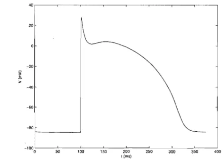
:> -40 -60 50 100 150 200 t (ms) 250 300 350 400

Figure l.1: Schematic diagra.m of transmembrane action potential for ventricular ceil.

The schematic diagram of the action potential is given by Fig. 1.l.

In normal cardiac cells, refra.ctoriness is primarily controlled by the membrane potential. The absolute refractory period coincides with the period when the membrane potential is more positive than the threshold potential. The relative refractory period, in which a higher stimulation current has to be applied to launch an action potential, corresponds fairly closely to the phase of repolarization when the membrane potential is between the threshold po-tential and the resting popo-tential. In sorne cardiac ceUs, the relative refra.ctory period is followed by a. supernorma.l period of enhanced excitability near the termination of repolar-ization. The excitability of ca.rdiac cells, assessed by applying electrical stimuli, has received considerable alteration. The strength, duration, and polarity of the applied current are aU important in determining responses. In general, the longer the duration of the stimulus, the less the intensity of current is required for excitation. For a fixed stimulus duration, the minimal stimulus required to pro duce an action potential is referred to as the stimulus threshold. relationship between current strength and duration for threshold stimuli is approximately hyperbolic. Certain cardiac cells, such as cells of the sinoatrial

(SA)

node, spontaneously depolarize to threshold potential to generate action potentials. Generally,

such automatic ce11s exist in the sinoatrial node, the atrioventricular (AV) node, the His bundle and the peripheral Purkinje network. There is considerable functional heterogeneity among these components; however, each has properties of automaticity and/or conduction that differentiate it from ordinary working myocardial ce11s.

1.2

Rhythmical Excitation of the Heart

In a normal beat, electrical activation starts from the

SA

node which propagates to both atria. It travels successively through the AV node, the His Bundle and fina11y to the Purkinje fibers that distribute the excitation around both ventrides

[9-11].

In human, when the system functions norma11y, the atria contract about one sixth of a second ahead of the ventrides, which a110ws the final fi11ing of the ventrides before they pump the blood through whole body [10,12]. Another especia11y important property of the system is that it a110ws a11 the tissue in the ventrides to contract in order to optimize the ejection of blood.

1.3

Arrhythmias

Genera11y human heart rhythm is considered normal if excitation originates in the

SA

node, is conducted through the normal pathway, and has a regular rate between 60 to 100 beats per minute [12]. But this simple definition, although attractive, cannot account for the c6mplex-ity of a11 the cardiac rhythms. According to the standard definition, sinus rhythm less than 60 beats per minute should be regarded as abnormal. But young adults, particularly athletes, frequently display resting heart rates of 40 beats per minute or less, often with intermittent junction escape rhythms and occasiona11y with AV nodal block [13]. Children and young adults may also manifest irregular heart rates that may be seen as sinus arrhythmia but that, on doser inspection, has no pathological significance. In contrast, these same rhythms in the symptomatic elderly patient are frequently manifestations of serious underlying diseases. A low sinus rate can also suggest an underlying pathology such as hypothyroidism.

than 100 beats per minute is a1so regarded as abnormal, it may be a normal response to stress. In fact, aH cardiac rhythms must be evaluated in the clinical settings in which they are seen. Any evaluation of the significance, untoward effects, and treatment of a disorder of cardiac rhythm is inadequate without the relevant clinical information.

The abnormal rhythm of heart beat is called arrhythmia. This is the most common term and it has become widely accepted, despite the fact that it erroneously suggests an irregu-larity of the heart beat. On the contrary, many of the arrhythmias have an entirely regular rhythm as, for example, paroxysmal atrial tachycardia, atrial flutter, ventricular tachycardia, complete A V heart block, and others. The term is dysrhythmia. arrhythmias can be classified among three groups according to their mechanisms: of impulse formation (Le., those caused by abnormal automaticity), disorders of impulse conduction and disorders produced by abnormalities of both impulse formation and impulse conduction

[12J.

1.4

Reentry

Tachyarrhythmia is commonly produced by reentry. Reentry is self-sustained propaga-tion of an activapropaga-tion front in an excitable medium. The onset of reentry requires sorne form of unidirectional block within a conducting pathway. Furthermore, the effective refractory period of involved action potentials plays a major role in determining whether or not a reentry circuit becomes established

[4,12].

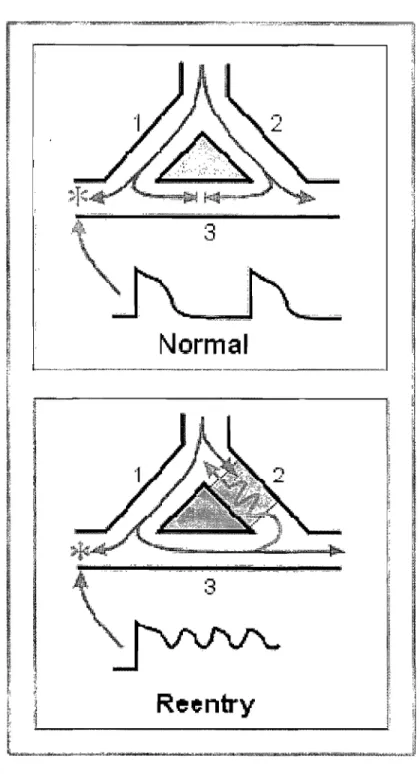
The reentry is the highest proba.ble mechanism of ventricular tachycardias (VT) occurring during the chronic phase of myocardial infarction. It is also the mechanism for atrial flutter. Fig. 1.2 illustrates the requisite conditions for re-excitation by means of a re-entrant circuit. First, a barrier must exist in order to form a circuit. This barrier could be an anatomical or functional obstacle. In the case a ring of tissue, the barrier is the central hole. Second, the conduction time around the ring must exceed the refractory period. In the case of normal cardiac muscle, the long refractory period makes reentry difficult. A locus of abnormally slow conduction may help sa,tisfy the requirement that the transit Ume exceeds the refractory

Normal

Reentry

Figure 1.2: Schematic diagram of reentry. Top panel: normal propagation, the excitation propagates through branches 1 and 2, and dies out at position 3. Bottom panel, the branch 2 acts as a site of unidirectional block. When the excitation front comes, the branch 2 is refractory and the excitation only propagates from branches 1 to branch 3. Excitation can then be conducted in branch 2, if it has regained its excitability. If branch 1 is again excitable when the excitation front exits from branch 3, a reentry is established [4].

period of site that is l'c,-av'-" [4,12]. In normal propagation, shown in the top panel of Fig. 1.2 the excitation propagates through branches 1 and 2, and dies out at position 3. In the bot tom panel of Fig. 1.2, the branch 2 acts as a site of unidirectional block. \iVhen the excitation front cornes, the branch 2 is refractory and the excitation only propagates from branches 1 to branch 3. Excitation can then be conducted in branch 2, if it has regained its excitability. If branch 1 is again excitable when the excitation front exits from branch 3, a reentry is established.

Even if it represents an oversimplified experimental model of clinieal tachyarrhythmias, the study of reentry in rings of eardiac tissue have allowed a careful analysis of a. variety of dynamic events that are relevant to ventricular tachycardia occurring around an inexcitable obstacle as weIl as atrial flutter [8,14-16]. a complete understanding of the spatial and time properties of the phenomenon, however, there serious complicating factors, such as the anisotropie tissue properties, the spatial in membrane properties and cellular interconnections.

1.5

Beeler-Reuter-Roberge-Drouard Model

of the

Car-diac ventricular myocyte

1.5.1

Description

Different mathematical models of the electrical properties of ventricular cardiac myocytes have been proposed, they differ in the number of ionie meehanisms that they include [17-20]. In our study, we used the Beeler-Reuter model, as modified by Drouard and Roberge [18,20J. We chose this model because its dynamic properties were thoroughly established both in the space-clamped and continuous one-dimension al ring configurations. Since our goal was to contrast the dynamics in the continuous and discrete one-dimensional loop, we have decided that this was an appropriate choice to analyze the changes specifically indueed by discrete intercellular gap junction resistance.

the excitatory inward sodium current,

i

_{Na ,} a slow inward calcium current, iCa, assumed to be carried by calcium ions, and , a K+ outward current. There is also an additional time-independent outward potassium current, i_{k1 ,} exhibiting inward-going rectification. The

iNa. primarily controls the rapid upstroke of the action DotelltI:!l.l while the other currents determine the configuration of the plateau and the repolarization phases. In the space-clamped configuration, the variation in membrane potential (Vm , in mV) is expressed by the relation:

dVm 1 (' . . .

dt

= -

Cm ~kl

+

~xl

+

~Na

+

~Ca (1.2)

The membrane current density is expressed in fLA/ cm2

, while the membrane capacity

Cm is set at 1fLF / cm2) the generally accepted value for the capacity of biological membranes

Cm [19,20]. _iext corresponds to a stimulus current that can be injected in the internaI medium. The scaling of the individual ionic current is chosen to provide éurrent-voltage relationships which match the best estimates obtained experimentally and taken together, pro duce an acceptable shape for the ventricular action potential. The individual Ionie currents (iNa) are given by the relations:

(1.3)

where gNa

=

15mS/cm2 is the maximum conductance of the sodium (mS/crn2 = 1/ Kn/crn2) and where ENa is the Nernst potential associated to the Na+ ions (fixed at -40mV). The state of each sodium channel is controlled by three types of independent gates that can be open or close: one activation gates (m), and two inactivation (h and

j).

The variables m, h, and j represent the proportions of each type of gates that are in the open state.

The individua.l ionic currents (ica) are given by the relations:

(1.4)

where gCa = 0.09mS/ crn2 is the maximum conductance of the calcium, the cl and

f

are the proportion of the activation gates and inactivation gates of the Ca2_{+ channels in the open}

state, respectively. Eca, the calcium Nernst potential, varies with the internaI concentration

of [Ca] (mM) according to the relation:

ECa

=

-82.3 13.02871n[Ca] (1.5 )

The dynamics of [Ca] is described by the relation:

(1.6) The time dependent activated outward potassium current ixl is given by

(1.7)

where Xl is the activation gate variable and Zxl is given by -: 0.8{ exp[0.04(~n

+

77)]- 1}

~xl

=

exp[0.04(~n

+

35)] (1.8)

The time-independent potassium current exhibiting inward-going rectification (ik1 ) is given by

o

035{ 4(exp[0.04(Vrn.

+

85)]- 1)

+ _ _

~_

... _-:---'----:-:::} ( )

. exp[0.08(Vm

+

53)]

+

exp[0.04(~n

+

53)] 1 _ ' 1.9

the dynamics of the gate variable m, h, j, d,

f

and xl is described by the relation

(1.10) (1.11) where Yoo and Ti are related to the rate constants of the transition from close to open state (a) and open to close state ((3) by the relation

1

Ti=

-ai

+

(3i

The voltage-dependent rate constants a and (3 are given by

a((3) = Clexp[C2(~n

+

C3 )]

+

C4(Vm.

+

C5 ) exp[Cô(Vm

+

C3 )]

+

C7

(1.12)

(1.13)

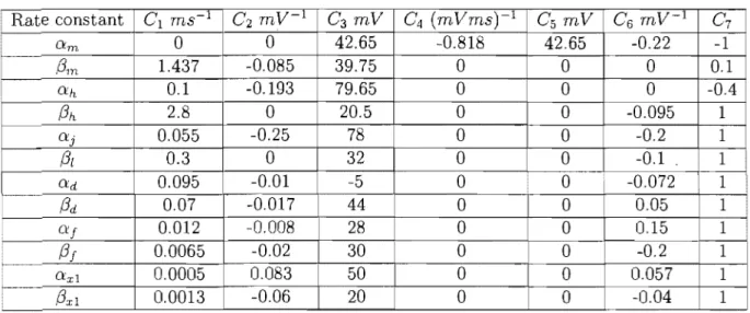
Table 1.1: C, defining function and values for rate constants

(0:

and (3) Rate constant

Cl

ms-1 _C 2 m C3 mV C4 (mVms) 1 C5 mV C6 mV-1 C7 O:m 0 0 -0.818 42.65 -0.22 -1 /3m 1.437 -0.0 0 0 0 0.1 O:h 0.1 -0.1 0 0 0 -0.4

/3h

2.8 0 0 0 -0.095 1 O:j 0.055 -0.25 78 0 0 -0.2 1 /3/ 0.3 0 32 0 0 -0.1 1 O:d 0.095 -0.01 ·5 0 0 -0.072 1

/3d

0.07 -0.017 44 0 0 0.05 1 O:f 0.012 -0.008 28 0 0 0.15 1

/3i

0.0065 -0.02 30 0 0 -0.2 1 O:xl 0.0005 0.083 50 0 0 0.057 1

/3xl

0.0013 -0.06 20 0 0 -0.04 1

by table 1.1. The dynamics of these gates variables fo11O\v the formulation first proposed by Hodgkin and Huxley [19]. Using this approach, with a fixed membrane potential Vm , the proportion of any specifie gate

popu-lations in the open state converges toward a voltage dependant steady-state _{Yi,cx,(Vm) with} a characteristic time constant Tlv~n). If Yi,=(Vm ) is small at low

V

m values and increased

toward 1 as Vm is increased, the Yi gate is said to be an activation variable, and is called

an inactivation variable in the inverse case. Typica11y, the value of the steady-state and· time constant function of the gate variable are obtained by fitting the experimental results obtained using the voltage-clamp technique [19]. In essence, this technique involves abruptly changing the transmembrane potential from an initial value to a predetermined clamp po-tential and maintaining this clamp popo-tential constant by the injection of a feedback current despite changes in the membrane conductance. It involves different procedures in order to isolate the contribution of a specifie current, as weIl as multistep protocols to obtain char-acteristics of the activation and inactivation gates when they contributed together to the dynamics of the current [21,22].

1.5.2

Dynamics on the Space-Clamped

M

BR

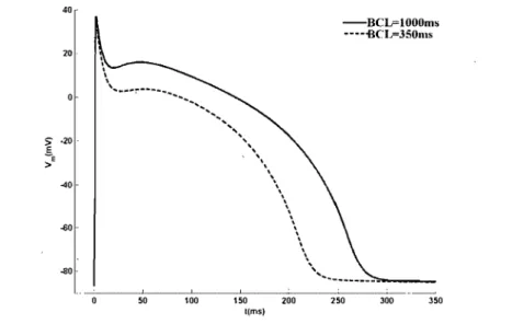
The Figure 1.1 shows the action potential obtained from the M BR model stimulated from rest by a square current pulse of 1 ms. The dynamics of the space-clamped M BR model have been studied both for the presence of constant bias currents and repetitive pacing with square pulses of current. In the case of the constant bias current, it was shown that there was an interval over which the model is automatic, producing repetitive action potentials [23]. However, the results obtained with pacing are more relevant to the present work on reentry. For pulse stimulation, the response of the M BR model is aU or none [24]. If the current is below a threshold, it produces a small passive depolarization and repolarizes as soon as the stimulus is removed. If the stimulus is ab ove the threshold, it produces an action potential as in Fig. 1.1, whose duration does not depends on the intensity of the stimulus above the threshold. This can be seen in the Fig. 1.3, which shows the stable entrainment response of the model to 40

pA/

cm2 _{square pulses of current of 1ms duration applied at two}

different basic cycle lengths (BC L = 1000 and 350ms). In both cases, the system produces a stable period-1 repetitive response with fixed action potential duration (A) and diastolic interval (D) that it reaches after a transient period at the beginning of pacing. During the plateau of the action potential, the slow inactivation variable

J

controlling ica. closes, and the slow activation variable Xl of ik opens, both contributing to the repolarization. Then, these

gates variables return toward their respective resting value during the next diastolic interval. However, as BCL is decreased, they do not have the time to recover completely, leading to a buildup of the Xl and a graduaI decrease

J,

which lead together to an abbreviation of the action potential duration. Period-1 response corresponds to an equilibrium, where Xl and

J

reach a mean value such that the changes occurring during the depolarized phase are exactly compensated by the recovery during the next diastolic interval.

The value of the threshold current

(Ithr)

depends on the duration of the pulse, and on the prematurity of the stimulation. The action potential duration is also a function of prematurity. As shown in Fig. 1.4, the prematurity can be measured by the time interval

40 . 20 >" ·20· E

;E

40·· -60--80· -BCL=lOOOms ---BCIp350ms .. ... : ... 1 ... .1 •••••••••••••••••••••••••• .1 ••••••••••••••••••••••••• _ ••••••••••••••••••••••••••••••••••••••••••••••••••••••••••••••••••••••••••••••• 50 100 150 200 250 300 350 t(ms)

Figure 1.3: The action potential duration is also a function of prematurity, This graph shows the stable entrainment response of the model to 40 muA/cm2ms square pulses of current of 1 ms duration applied at two different basic cycle lengths (BeL

=

1000 and 350ms). The

duration of the action potential is reduced when the BeL, which is the time between the successive stimuli, becomes shorter [23].

between the onset of the new stimulus 52 and that of the prevlOUS stimulus 51 having produced an action potential, the so-called 52 - 51 interval. Alternately, prematurity can also. be measured by the diastolic interval D, consisting of in the time span between the end of the previous action potential and the onset of the new stimulus 52. For the AI BR model,

the action potential duration

(A)

is defined to end at the moment when

V

m reaches -50

m V in repolarization. The restitution curve, giving the duration of the action potential as a function of the prematurity of the stimulus, provides a global picture of variation in the action potential duration. As illustrated in Fig. 1.5, the restitution curve can be constructed by first obtaining stable entrainment of the system for a given BeL pacing, and then applying 52 stimuli with a varying prematurity on the reference action poteiltial. The duration of the resulting action potential for each value of the 52 - 51 interval are recorded.

Fig. 1.5 shows the restitution curves obtained after a pacing of BeL at 1000.and 350ms,

of which stable responses are displayed in Fig. 1.4. The two restitution curves are different because the action potentials after which 82 is applied are different. The action potential

11<: L=1OOOms D

---1

nCL=350ms D

---

---~

n'----_ _ _ _

----'n

51 52

Figure 1.4: The two different basic cycle lengths

(BeL

=

1000 and 350ms). Two stimuli

SI

and

S2

applied [23].

duration ofthe stable entrainment response at

BeL

=

350ms is much shorter than the action

potential obtained at

BeL

= 1000ms. In consequence, the absolute refractory period at

BeL

=

1000ms is longer, as the minimal

S2 - SI

interval to obtain an active response is longer. The two restitution curves expressed as a function of

S2 - SI

appear to be shifted, relative to each other. However, as seen in the right panel of Fig. 1.5, the two curves are almost identical when

A

is expressed as a function of the diastolic interval

([S2 - Sl]-

As,

the

As

of the response to pacing). In reference [23], it was shown that the

A(D)

restitution curves of the l'vI BR model were almost identical for reference action potentials obtained from

a wide range of pacing frequencies and durations of square pulse stimulation. It was also shown that

Ithr(D; Tpulse) ,

the variation of threshold current as a function of the diastolic interval for each duration

Tpulse

of the square pulse stimulus, was also an invariant function for each duration. Memory effect, by which the threshold and/or the A would depend not only on the last action potential but also on the preceding sequence of activations, can therefore be neglected in the standard

1\11 BR model. However, it was shown that for sorne

A(ms) 250 -llCL=IOOOl11s 150 50 200 ----·BCL=350ms -",., .... ,. ... " 1 1 1 1 1 : : :

/",_.

,-"

1

1

!

, J , 300 400 S2-SI (ms) 500 1\(I11S) 250 150 50 o 100 200 300 D(l11s)

Figure 1.5: Action potential duration

(A)

obtained by premature stimulations of the stable response at two BeL. S2 - SI is the time from onset of the last pacing stimulus to the premature stimulation. D is the time from the end of the action potential to the onset of

the premature stimulation. Left panel: A changes when expressed as a function S2 - SI. Rigth Pannel: When A is expressed as a function of D, the two curves merge, showing that A only depends on D [23].

the memory effect could no longer be neglected [25,26].

As it will be explained below, the invariance of the A and It1~T curve as a function of D permits understanding of the change in entrainment response with respect to the frequency of stimulation. Fig. 1.6 shows the stable entrainment response of the model to 40pA/ cm2

square pulses of current of Ims duration applied at different BeL.

In

each of the two top panels, aU stimuli produced the same action potential. This entrainment can be caUed a 1: 1 response, meaning that each stimulus pro duces the same active response. However, as expected, the duration of the action potential is reduced when the BeLis shortened. The two subsequent panels, with BeL

=

265 and 260 ms, show another type of entrainment where each stimulus still produces an active response, but with duration alternating between a long and short action potential. This can be caUed a 2:2 entrainment, meaning that the periodic pattern of response repeats after two stimuli and induces two different active responses. Finally, at a shorter BeLin the bottom panel, the pattern of response still repeats

o~~---_

-50

1-

--~-'

- _

... _

-100- _BCL=270ms

r

I"--

t\ ~ 1:1

-5~ ~.---~"

I---~···~

1

---~

__ ..

_I-..

---...~

~_~

_._ ... _....J 100 - BCL=265ms . ~ ~ 2:2

-5~~---~·_~r---~_

..

J

---~~ ----~"-_

..

--

100-o[>----_~, ~

-501-

~

~

1

__

BCL=260ms

----~ 1~2:2

___ J ~ _ _ _ ..

·100-~

l

1\ BCL=260ms 0.. - . -.. - - - . 1'---~:1 -50 - _", _ _ . _ L - -

~-

...

T-~

.... _ _ L _ ....

_'---=:_Tm~

-100 0 1~0--200 300 40-0--50-0--600 700 800 900 1000 t(ms) ..

Figure 1.6: The first and the second rows show 1:1 response, the third and the forth rows show 2:2 response and the last row shows 2:1 response.

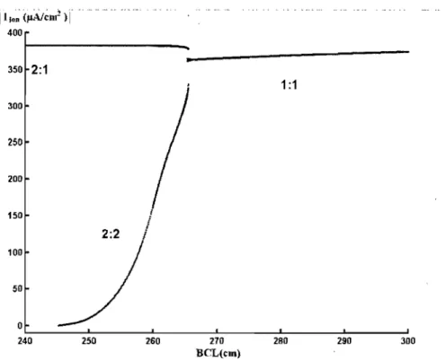
after two stimuli but each periodic sequence contains an active and a passive response, a rhythm that can be called a 2:1 response. Fig. 1.7, showing the maximum inward current following each stimulus, provides a synthetic view of the bifurcations.

Fig. 1.8 provides a schematic representation of the dynamics for producing successive stimuli that provoke an active response during pacing at a fixed

BCL. Di,

the diastolic interval preceding the onset of the ith stimulus, is equal to

BCL -

Ai-l, where A i- l is the duration of the action potential produced by the stimulus i - 1. Since

A

is only a function of the diastolic interval, this relationship leads to the finite-difference

(F

D) equation:

(1.15)

A 1:1 response corresponds to a fixed point (i.e. Di

=

Di+l

=

Ds)

of the system and is stable if and only if

(1.16)

Illon <llA1~It1!

)1

400 350 2:1 300 250 200 150 100 50 o

...

1:1 2:2 ~ _ _ _ _ - L _ _ _ _ _ _ ~ _ _ _ _ ~~ _ _ _ _ - L _ _ _ _ _ _ ~ _ _ _ _ ~ 240 250 260 270 BCL(cm) 280 290 300

Figure 1.7: The maximum inward current

(IIion(flA/cm

2

₎₁₎

_{following each stimulus provides}

a synthetic view of the bifurcations.

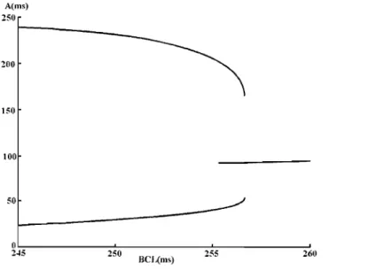
A(llls) 250 200 150 100 50 ~~':-:-5---:-2~50---:2~55:---:-'26-0 BCL(ms)

Figure 1.9: The finite difference model reproduces the bifurcation of the

AI BR

model. The model was simulated using A(D) function fitted from Fig. 1.7.

that the 1: 1 response loses its stability when A and D faH on the portion of the restitution curve where the slopes are greater than 1. Fig. 1.9 presents the bifurcation from 1:1 to 2:2 predicted by the F D model, with A( D) fitted from Fig. 1. 7. It reproduces the nature and the position of the bifurcation obtained in the M

BR

model. In fact, the F D model, complemented by rule to account for the threshold and the absolute refractory period, has also been shown to correctly reproduce the complex bifurcation structure, appearing with respect ta the

BCL

and the amplitude of stimulation. However, as we shaH see in the next section, the bifurcation from 1:1 to 2:2 response is the most relevant with respect to reentry.

1.6 Modified Beeler-Reuter Loop Model

The bifurcation from 1:1 to 2:2 response observed as the frequency of pacing is increased in the space-clamped M

BR

model suggests that transitions may also occur during reentry. Much work has been do ne on reentry in a one-dimensionalloop, using either ionic models or low-dimensional representations of the dynamics [25,27-36]. Most of the studies using ionic models have used the cable equation, which considers the membrane as an homogeneous

and continuo us cylinder, the extracellular medium as an equipotential and neglects the radial current in the intracellular medium [21]. With these hypotheses, the evolution of the membrane potential V on a loop of length L is described by the partial differential equation:

~

82Vi(x, t) _~

=

S[e. 8Vi(X, t) Ii ( )] XE[O, L]

2 ln ~

+

ton X, t ,

P uX ut (1.17)

with the boundary condition

V(O, t)

=

V(L, t) (1.18 )

where p (KD·cm) is the constant axial intracellular resistivity, Cm (p,F/cm2

) is the membrane

capacitance and S (l/cm) is the ratio of the surface of the membrane to the volume of the intracellular medium. Iion(x, t) is the ionic current crossing the membrane. For the M BR

model presented in the previous section, the dynamics variables (Yi, i

=

1,6) and [Cai]

become functions of space and time in such a way that their equations must be solved at each site of the membrane. There is no diffusive term for these variables, but they must fuI fi Il the boundary conditions (Yi(O, t)

=

Yi(L, t), [Cai(O, t)]

=

[Cai(L, t)]. Diverse numerical methods exist for solving this type of system [27,34]. We present here a numerical method devisecl for parallel processing [27]. This method is described in Appendix l of this thesis, we have modified for the loop with dis crete gap junction resistances. The loop is first divided in a number of segments

(j

=

1, N) of length Le and the system is solved with a constant

i '

time step 6.t. For each time step, the system describes the spatial evolution of V within each segment at time t

+

6.t becomes an ordinary differential equation:

d2Vj(x,t+6.t)=pSCmVj ( J\)_pSCmVj ( ) SIj ( )

dx2 6.t x,t+ut 6.t x,t +p ton x,t (1.19)

Since aH the quantities at time tare known, this system is equivalent to: __d2_----'V J=--::-' (x----,) K2

vj -

j ( ) [ L ] ' - 1 N

dx₂ - - 9 X XE 0, e J - ... (1.20)

With the boundary conditions:

V1(0) V N (Le), (1. 22) dVi(O) _dVi-1(Le) j = 2,N-1 (1. 23) dx - dx dVl(O) dVN (Le) (1. 24)

=

dx dx

conditions assure the continuity of the voltage and of the axial current between the loop.

The solution of Eq.(1.20) is given by the sum of a particular solution

V;

and of the solution

Vk

of the homogeneous system;

(1.25)

The

V;

is obtained by solving Eq.(1.20) for each segment with the Neumann boundary conditions:

(1.26) To obtain this particular solution, each segment is discretized with a constant spatial step of .6.x and the is solved by using a linear finite element method [34]. Then the segments are reconnected by calculating the Aj and Bj to fulfill the continuity conditions. Reentry can be initiated by disconnecting the loop, stimulating one of the free ends and then closing the loop after a delay. Once reentry has stabilized, it is possible to shorten the loop gradually to investigate the effect of the circumference on the dynamics of reentry. Quan and Rudy [35] have shown that reducing the loop length results in an increased degree of head-tail interaction that, in turn, brings about shortening and eventually alternation in . action potential durations. Vinet et al. [27,28] as weIl as Courtemanche et al [30,31], working respectively with the Iv! BR model and the original BR model, have provided a complete study of the effect of the loop length.

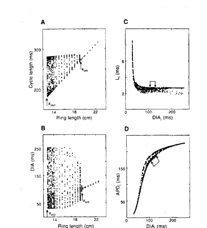
Results for the M BR model are presented in Fig. 1.10 (A). For each loop of length

L, measurements are taken at one site for multiple turns. a, long L, the cycle length, which is the time between successive acti0n potentials at the measuring, is constant. Moreover, the action potential duration (APD: from the of the upstroke to -50mV

downcrossing in repolarisation), the diastolic interval (D l A: from the end of the action potential to the next upstroke) are the same for aIl action potentials. In this case, the reentry is periodic (period-1) and corresponds to a fixed waveform traveling at constant speed around the loop. As the loop is shortened, the cycle length decreases because the speed of propagation remains almost constant. Both DIA and AP D also diminish, they take place in a space-clamped membrane when the pacing frequency is increased. Then, below a critical length Xcrit, the cycle length, DIA and AP D become multiple values. At Xc.rit , the cycle length has exactly the value for which there is a transition from 1:1 to 2:2 response in the space-clamped model. However, the response is not 2:2 in the loop but rather wanders between an upper and a 10we1' bound. These bounds part as L becomes shorter, until a minimum Xmin below which sustained reentry becomes impossible.

To get a clear picture of reentry below Xcrib propagation must be followed as it proceeds along the loop, recording successive AP D and DIA values at each site. 1.11 shows the spatial variation of DI A along the loop for successive turns abutted end-to-end. There is a spatial oscillation of DIA as propagation proceeds, with a wavelength that is an irrational fraction of L. Hence, the sequence of DIA measured at one site becomes quasiperiodic (QP).

As shown in figure l.I1, two different types of QP reentry were observed on the MER loop, one with a wavelength close to 2L, and a second with a wavelength close to 2/3L.

Courtemanche et al. [31] have extended the

F D

model that was developed for the paced space-c!ampe. As for the F D model, AP D is assumed to be a function of the previous action potential, which yields

(1.27) where DIA(x) stands for the diastolic interval of the ith action potential at site X, and

C Li

(x) is the cycle length between the new activation and the previous one. If the successive turns are abutted end-to-end and X is extended to span multiple loop length L, DIAi_l(X)

_300 li)

g

250

-

(/) E

--<Ct CI 150 50

A

B

14 18 22 Rîng length (cm)

Ii".'" .' .

~i"!\ •• : •

~

_:

_...

f.

_.

, .1 ••

.

_...

-.

_..

_""

_...

.

.

~

.

, • • r • 1. l..f1 .: . . t · ••• ... '" •• " • t • J

V-." "

l • t • •• rlJ". ~ ••

Il.

_!

{(o"'" : • ' ' • t4~: . • ,' ""

,1'

.:'\l~ ... :. • •.

-1. .'

l'· :::'

• : ;

j-Ir"

I;i

-•• '.. J".

i ; ;

~

:;;1

t

:, l , t •

txm'J'

14 18 22 Ring length {cm)

c

6

-

o E

---2 ~---~---~--_{100 200}

o

DIA_I (ms)

D

150

--

li) E

-50

o

100 200 DIA_i (ms)

Figure 1.10: Analysis of temporal activity recorded at a single point on rings of different

lengths. (A and B)

CL

and

DIA

for a maximum of 25 successive turns at each ring length.

Stable reentry occurs for X

>

Xcrit

=

19.6cm,

complete block for X

<

Xmin = 12.8cm,

and

irregular propagation for

12.8cm

<

X

<

19.6cm.

(C and D) Scatter diagrams of latency and

APD

versus

DIA

for aIl patterns displayed in (A) and (B). Arrows in

(C)

and (D) indicate

the set of points corresponding to stable reentry (X

>

19.6cm) [27].

- - l ' j

f\

rr

1\

f\

250_1,

f-

ti&

('

200 1 11

l,

r

~

: \. ' 1

\

{ o~ " j

d

1

t

f

_i

₁₀₀ Il _Il

_{J \}

Il 'i 1 1 t l ~1~1 ₁ '~,

j

\

1 1 li! ! f

..,

\ i

\ 1

t

1

1

g'

1

il

:::l

)

1

J'

,1 _lOf.) 1

\ / \ 1

1

1

:

₁

/

! 1

\ 1

1

,

;' ~.o, l'

tl

, , /

./

1)

~i

V

V

1

50 1". ~ :2 <l :2 3 j Xl'1. :J,I\,

Figure 1.11: Mode-O at L = Xmin = 12.8cm, and mode-l at L = 18.65cm, MBR model [29]. delay equation:

DIA(x) = CL(x) - APD(DIA(x - L)) (1.28)

The last hypothesis, appropriate for the BR and M BR models, is that the speed of

propa-gation e is also a function of DIA. Then,

l

x 1

CL(x)

=

x-L e(DIA(y))dY (1.29)

and the complete model becomes an integral-delay equation:

l

x 1

DIA(x) = x-L e(DIA(y))dY - APD(DIA(x - L)) (1.30)

Courtemance et al. [31] have analyzed the stability of the constant solution (DI A(x) =

constant) corresponding to period-l reentry. They have proven that it remains stable until

DI A = DI Acrit where '

d(APD)

1 d(DI A) IDIACTit= 1 (1.31 )

Renee, the criterion for the stability of the 1:1 response in the paeed spaee-clamped model also controls the stability of the period-l reentry in the loop. Furthermore, they have also proven that an infinite number of quasiperiodic mode of reentry appears at the bifurcation, with wavelength

À

~

2L

[ l

The two modes of shown in Fig. 1.11 have a wavelength close to n

o

and

n

=

1 respectively, and are accordingly designated as mode-O and mode-1 reentry.

two modes were observed in the

BR

and

M BR

models. In both cases, mode-O reentry was shown to appear through a supercritical Hoph bifurcation. The amplitude of the spatial

DIA

oscillation grows from 0 as L is shortened below

Xcrit?

and reaches a maximum at

X

min ,

where sustained reentry stops. Vinet et al. [27] found that the mode-1 reentry to display a large amplitude at a length shorter than Xcrit and to disappear when L is larger than

Xmin . Higher modes (n

>

1) of propagation were never observed, even after a systematic

search for appropriate initial conditions [27,29]. Although successful in predicting the loss of period-1 solution, the integral-delay model could not explain the difference in the way mode-O and mode-1 are created, as weIl, the absence of n

>

1 modes goes unexplained. Vinet et al. also observed that the

AP D

vs

DI A

relationship was becoming dual value (Fig. 1.1 O(D)) in quasiperiodic reentry. They suggested that this was a consequence of the effect of coupling on repolarization, by which the surrounding of a point influences its repolarization and modifies the

APD

[29,37,38]. They proposed to include in the integral-delay model the effect of coupling on

AP

D through the equation:

APD(x)

=

fUuw(y)APDr(DIA(X+y))dy

(l.33)

where

APDADIA)

is the restitution curve as in the

DF

model,

w(y)

is a weighting function chosen as a normalized Gaussian (i.e. w(O) = 1), and u is the extent of the neighborhood influence. This led to the modified integral delay model

DI A(x)

=

l~L ()(DI~(Y))

dy - f: w(y)APDr(DIA(x -

L

+

y))dy

(l.34) As shown in Fig. l.12, the modified integral-delay model can correctly reproduce the bifur-cation structure of the

M BR

model as weIl as the multiple-value

AP D

vs

L

relationship observed in quasiperiodic propagation. FormaI analysis of the model [29,37,38] ruso shows that the coupling displaces the value of the loop Iength at which the mode is created and may forbid the appearance of higher modes. The study of bifurcation has been extended to

APD(llIs) ,,~ 150 19 .. 4 L(em) 1 1

Figure 1.12: Mode-O is represented by the solid line, and mode-1 is given by the dash line as a function of

L [29].

the two-dimensional ring, a more complex system due to additional contribution of curvature of activation and repolarization front to the stability of reentry [39-42].

1.7

Role of gap junction in the propagation of the

car-diac action potential

Real cardiac tissue does not form a syncytium as hypothesized in the cable equation. Rather, the tissue is formed by discrete myocytes electrically connected by gap junction resistances such the cell to cell propagation is discontinuous [43,44]. Gap junctions play an important role in the velocity and the safety of impulse propagation in cardiac tissue. Under phys-iologie conditions, the specifie subcellular distribution of gap junctions together with the tight packaging of the rod-shaped cardiomyocytes underlies anisotropie conduction, which is continuous at the macroscopic scale. During gap junction uncoupling, discontinuities reap-pear and are accompanied by slowed and meandering conduction. Junction resistance can -be modulated to obtain very high values in abnormal cases such as ischemia and infarction,

Figure 1. B: Gap junction in the series branches of myocytes from the most superficiallayer of the monkey's right ventricle (1660x). They consist of steps and risers [45].

leading to very slow conduction. In extreme cases, it may lead to complete decoupling of neighboring cells, resulting in a conductioll block. Fig. 1.13 shows an electron microscope picture of the gap junctions in myocytes extracted from a lllonkey's right ventricle.

The cellular structure of the myocardium is important for understanding both normal propagation and arrhythmogenesis. Structural anisotropy may be related to cell shape and also to the cellular distribution pattern of proteins involved in impulse conduction, such as gap junction conllexins and membrane ion channels. The functional connections bctween cardiac cells, consisting of so-called gap junctions, vary in their molecular composition, degree of expression and distribution pattern. Each of these variations may contribute to the specifie

propagation properties of a given tissue in a given species. The gap junction is formed by the junction of two connexin proteins, eaeh being embedded in the membrane of one cell. Fig. 1.13 presents a sehematic representation of a gap junction eonnexin protein. There exist different forms of connexin as Fig. 1.14 demonstrate [46-50]. Connexin 43 (Cx43) is the most abundant protein in the heart and is also present in many other organs. Cx43 ean