Application of the Wavelet Transform for GPS Cycle Slip Correction and Comparison with Kalman Filter

manuscripta geodaetica (1995) 20: 161-172

manuscripta

geodaetica

© Springer-Verlag 1995

Application of the wavelet transform for

GPS cycle slip correction

and comparison with Kalman filter

F. Collin

and R.

Warnant

Royal Observatory of Belgium, Avenue Circulaire 3, B-1180 Brussels, Belgium

Received 23 November 1992; Accepted 4 January 1995

Abstract

In the past, severa! authors introduced a method based on phase and/or code combinations of GPS

data together with a Kalman fil ter to solve the prob-lem of the cycle slips. In this paper, the same phi-losophy is used but a comparison of the results ob-tained with Kalman filtering and the wavelet

trans-form is performed. The wavelet transform is a

rather new spectral analysis method which is in-troduced in the second paragraph. The comparison

of the two rnethods is accomplished in severa! steps: first. sorne data points are removed and jumps are

simulated in theorical and real signais to test the capability of the wavelet transform to mode! the signal i.e. to recover the removed data points and to compute the value of the jumps. Then. the anal-ysis is performed on real cycle slips. This last study

shows t hat the wavelet transform and the Kalman filter are very complementary and give both correct values for the cycle slips.

1

GPS

cycle slip problem and

Kalman filter

1.1

Introduction

The P-Code dual frequency GPS receiwrs can pe r-form two types of measurements:

• Pseudoran~'=' ( P-Code) measurements P,(l)

with:

?;(/)

=

r· ~1,( l)

=pt/) -i- /;(1)

+

T(t)

+

c(~s-(1) -tiR( Il) where

- ôs

is tilt' ~att>llite clock f'>rror - li 11 _{is the recE'i ver clock error}

- i

=

1. ".! refers to the carrwr L 1 or I .,

t

is the ti me of the pseudorange measure-ment

c is the speed of light

è!..t; is the code signal time of transit from

satellite to receiver

pis the geometrical distance between the

position of the satellite at time of emis-sion of the GPS signal and the receiwr at time

t

- /; is the frequency dependent path

lengthening clue to ionospheric refraction

-

T

is the frequency independent path

lengthening due to tropospheric refr

ac-tion

• carrier beat phase measurements <l>;(

t)

<l>;(t)

=r<I>

f(t)

-

c{lr(t)

+

.\

where

=- (

~)

(p(t)- l;(t) + T(t))

+f;(

o

(t)-

o

5(t)) + .V;

r<I>f

ts the phase of the L; carrier re -ceived from the G PS satellite by the G PS

recel ver

<l>r

is the phase of theL; reference signal generated by the receiver

- N; is the unknown inte_ger ambiguit.y in -herent in the GPS phase observations - /; is the nominal

L;

carrier frequency This mathematical mode! of the G PS obser

v-ables is very simple: it is valid under the assumpt!on thaL the receiver and satellite reference frequemie~ are wnstant with time . .-\ccept.ing this assumptic•n does not arfect the rcsults of this pap~r . .-\ mor~ complete mode! can lw found in Kin~ c'1 al.( 19~-;-· ..

G PS receivers continuously monitor the carrier beat phase <I>;. \\"hen they !ose lock on a satellite, an unknown integer n~mber of cycles is !ost. This

event is called a ·cycle slip'. These cycle slips have to be recovered in order to compute accurate posi-tions.

The first step in the cycle slip correction consists in setting up a test quantity which is a combination

of code and/or phase measurements. This co mbina-tian has to be a slowly time varying function so that a jump in this function will indicate the occurrence

of a cycle slip.

A first approximation of the cycle slip is com-puted using two phase-code combinations PC;

(uni ts of cycles):

PC;(t)

=

(<I>;(t) + (

~)

P;(t))

-(

<I>;(to)

+ (

~)

P;(to))

=

2 (

~)

(I;

(t)

-

1;(10 )) where 1₀ is the time of the first measurement. This function describes the evolution of the ion o-spheric refraction etfect since the first measurement. If a cycle slip of .;;,.V; cycles occurs. it will give rise to a jump

D..X;

in the beat phase <I>; but not in

the pseudorange

P;.

As a consequence. this cycle slip will result in a jump l::..N; in the phase-code combination PC;. When such a JUmp has been

de-tected. a first approximation of the cycle slip can be

computed using the fact that L:::..N; has to be an

in-teger number. l"nfortunately, the noise leve! of the pseudorange measurement obtained with the best P-Code receivers is of the order of one

L;

cycle for

ele\·ations above -!.)degrees. Larger values (.5 to 10

cycles) are obserHd in the case of multipath, Anti-Spoofing, and for low elevations. As a consequence. this method only gi v es a first approximation of the JUmp.

The final correct ion is obtained by us mg ;1

L 1 / L:. rombination PP:

lt ran be easily ~r-en that the occurrence of a cy-cle :;]ip (.::,.JV1, .::,..\":.!) will gi\·e a jump .::,.pP in the

L

1/

L:.

rombinati<)U:

l::..PP

=~

N

t-(;:)

D..

N2

(1)

The precision of the carrier beat phase measur

e-ments ( <I> 1) is of the or der of a few millimeters. This

means that the resolution of this method is much

better than the previous one. The disadvantage of

equation (1) lies in the fact that it contains two un-knowns

D.N

1 ,

D..N2.

Theorically this equation can be solved by using the first approximation given by the phase/ code combination. In practice, a dis-turbed ionosphere. a low elevation angle, the multi-path etfect can seriously degrade the usefullness of this method. A more complete description can be found in (Bastos and Landau, 1988; Landau. 1989:

Lichtenegger and Hoffmann- \·Vellenhof, 1989).

1.2

Kalman Filtering

In fact. in arder to be able to detect a JUmp, we have to compare a predicted value of PP (or PC,) with an observed one. Hence we need a mathemat-ical method to mode! the evolution of PP (or PC, )

versus time.

The above mentioned authors make use of the following discrete Kalman filter (details in Gelb. 19ï4: Bastos and Landau, 1988):

System and measurement models:

xk ~k-txk-t+Wk-1

;Ik H k X k

+

l::;.;

State and error covariance prediction:

X.,(-

)

E

k(

-

)

~-~xk-1(+)

~-1 Pk-t(+l~Ll

+

Q,_l State and error covariance update:

Xd+l

Ed+J

[( k

with:

X k the st<tte vector

'É_k the transi ti on mat rix IV k the state prediction error

H k the matrix forming the observation equations

E

k

the covariance of the state vector

Z.k

the vr-ctor of obst'rvations

.l.k

thE' measuremen t err or

1.

the identity matrix

l\. k the Kalman gain mat rix

0

the state transition noise matrix -=-k '

Ek

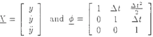
the covariance matrix of observations

The state transition mode! and the state transition

covariance matrices are taken from Bastos and

Lan-dau

(1988):

!:::..t 1

0

~t

!:::..t

l

1

with

::.t

,

the sampling rate, y,

y

,

jj the considered

combination

(PC;

or

PP)

and its derivatives. Phase/Code combination:

[ 10-8

Q=

0

0

0

10-10

0

0

0 10-12

\\'e use the elevation dependent measurement noise mode! given by Eueler and Goad

(199

1

)

for a Rogue Receiver : w he re h is the elevation angle. Ph<1.se combination:

Q

= [

10-~ 0 0

0

10-

8

0

0

0

ro-

to

][

R(cyc/es2)

=

.)10-

4 cycles2 ] cycles-2

ln the next section. we will compare the results ob -t ained by using this Kalman fil ter and the wi\velet

transform.

2

Introduction to

the

wavelet

transform

The 1\'ilVclet transform is born 6 years ago when

scientists realized that the fourier transform didn ·t

answP.r al! the questions about the frequency anal-ysts.

To detect the frequencies present in a signal. Fourier projects this signal on trigonometrie

func-tions 1 sine and cosme) and their harmonies. \\ïth t.he ~ame goal. the wavelet trélnsform

projf?rtS the signal on a family of functions ( named

wavPiets and noted g,,b(t)) issued from a basic fune

-r ion tnoted g(l) ) by dilatation (of factor '1z'- callt'd

the scale) and translation (of factor 'b'. called the

time parameter). Formally the relation between

!lab(t) and g(t) is: gab(t)

=

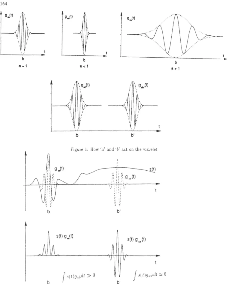
g( t~6).

Figure 1 shows how the parameters

'a'

and 'b'

act on the basic wavelet.

When

'a'

raises the wavelet stretches itself: the analysed part of the signal is larger and the wavelet essentially searches for the low frequencies. When 'a' decreases the wavelet contracts itself and a

smaller part of the signal is considered. In this case the wavelet detects the high frequencies present in the signal.

The parame ter

'b'

shifts the wavelet over al! the signal; this corrçsponds to a translation in time.

The coefficients of the wavelet transform

5(

a,

b

)

of a signal s(

t)

are gi ven by :

S(a, b)

=

j

gab(l).s(t)dt

(2)

Generally the wavelet transform is a complex

function of

'a

'

and 'b'- Therefore the information

about the signal is included in the modulus and in

the phase of the wavelet transform.

The use of the wavelet transform can be

summa-rized as follows: a basic wavelet (g(l)) is choosen. it is dilated of a factor

'a'

and translated of a factor 'b' (gab(l )) (see figure 1 ). Then using equation (2).

the signal is projected on flab(l) giving the result

S(a, b). \\'e make this operation for all the values

of 'b' ( shifting the wavelet over ali the signal) and for all the values of'a' (searching for all the

frequen-cies) to ob tain the wavelet transform of the signal. While Fourier only gives the frequency co

mpo-sition of a signal with the assumption that ail the

component frequencies are present from the origin

to the end of the 'infinite' signal. the wa\·elet

trans-form gi\·es the time location of each frequency. it

allows the visualisation of transient frequencies. the analysis of the law of dispersion ami the dete

rmina-tion of the occurrence of discontinuities in a signal.

This new method of analysis has bet>n applied

to a widt> range of physical problems: \'uclear \lagnetic Resonance spectroscopy (\!an ens.

1089:

G

uillcmain et al.

.1%9),

syn thesis of audio-soumis

1 Guillemain et al.. 1091 ), galaxy counts 1 ')lezat ~t

;Jl.. 1090). ;;tudy of multifractals 1 .-\rne·Jdo et al..

1088)

.

.:t.stronomy (Bijaoui et al..

10PI

J

.:~nd many

':

b

a-1 ' ' ' '

:

~ ' ' ' '

b

a<

1

/ \.g.Jt)

'

.

:

.

'

.

:

b :

/

\ 9.,.(t)

'

.

.

..

' b' ' ' Figure 1: How 1

a' and 1 _{b' act on the wavelet}

.

'• ,,

::

g

..,(1) b

b

., '• s(t)

g

_..,

(t) ,, '• ,,

:":

:: :':

g

(t)

!~I~i~_

.tt

·

·

.: \!

\

i

·

..

:

' 1 . ;

j

\!

b'

s(t)

g

(t)

"'

b' b B > 1

figure :! : Effcct of time-scale fil ter of the wavelets. ln the first part of figure 2, a signal s( t) is represented.

The da.,;hed line shows a wavelet for

t

=

b

and

t

=

b'.

The second part of figure 2 displays the wavelt't

2.1

Proper

t

ies of the wavelet trans-

The basic idea of this work is based on this

be-form

haviour of the modulus near a discontinuity. I n-For simplicity. the following properties are given

without any complicated mathematical Jemonstr a-tion. The evolution from the Fourier transform to

deed, when this kind of behaviour is obsen·ed in the wavelet transform of a signal, the presence of a discontinuity will be deduced.

the wavelet transform and the mathematical just ifi-cations of the wavelet transform can be fou nd by the

3

readers in Daubechies

(

1

992

)

,

Chui

(

1

99

1

),

Combes

(

1

988),

i'v!eyer

(1992),

Grossman et al.

(

1

99

2)

.

Cycle slip detection using

the wavelet transform

2.1.1 Zero mean of the wavelet

The wavelet must have zero mean, so that the pr o-jection of a signal dissimilar to the wavelet is al -most zero

(1

S(a. b) 1~

0)

and the projection of a signal similar to the wavelet has a large amplitude

(1

S(a.

b

)

1>>

0).

This is an effect of the time-scale filter: the wavelet (!lu b ( l)) only sees th at part of the signal which it resembles (Figure 2).

The wavelet used to detect the cycle slips is built from this idea. The Doppler effect present in the

G PS observations (due to the fact th at the sate l-lite is moving with respect to the receiver) leads to

a parabolic wal.k of the signal. We will build the wavelet so that it will "see" the discontinuities in the

G

P

S

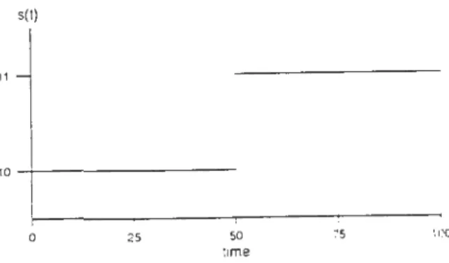
signal but not this second arder walk. 2.1.2 Wavelet transform of a signal with a

discontinuity

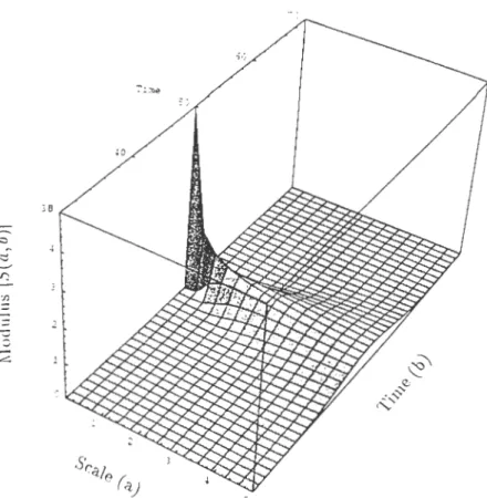
Figure 6 shows the shape of the wavelet transform

of a signal s(l) with a discontinuity in

t

=

.50

as presented in Figure 3. s(t) 0 25 50 ume 75 lOO figure

:L

Sit;nal with a discontinuity in

t

=50

lt appt"ars that:

The modulus of :hf tcareld lran8[orm 1s riwxzmum ru·ar the ril.sr.ont::w!ly. c;ro~sman et al .. ( l !)!)2).

3.1

Construction of the appropriate

wavelet

Owing to the fact that the wavelet detects only parts of the signal similar to itself, a wavelet which looks like the discontinuities encountered in the

GPS observations was built (Figure 4). Figure 7

shows such a discontinuity in the phase combina -tian

PP.

1

i Figure -1: Original \Vavelet Figure;): Final \\'avelet

165

figure 6: :Vlodulus of the wavelet transform

IS(a,

b)l

of a signal

s(t)

with a discontinuity in .)Q.

IS(

a.

b)l

grows for

a

-

0

and as a function of

b: IS(a, b)l

is maximum near the discontinuity.

pp

(cycles) \Va n'let Transform 2C: .GC ~ j j

o

.cc

-~ ~ GPS Time ""

-

22

.

0C

~.--~---~----~

:·::ooo

c:. Î r::. -.~-,-. ...,.l.t.... .... - ·- '-'

Figure ï: Cycle slip in the PP Combination

4.00

l

1,

O.OC

...!

~

~

_{Ti me}

-

4

oc

s

·

sooo

:20COO

5

:5

-JOO

530000

535000

1-'igure ,): \lodulus of the Wan•let transform of the signal displayed in figure ï. The occurrence of a cycle

This original wavelet was adapted in order to elim -inate the artefacts introduced in the wavelet trans-form by the parabolic behaviour of the signal (as mentioned before). Indeed, the GPS carrier beat phase has a parabolic behaviour due to the Doppler effect. The original Wavelet was built to detect jumps versus an horizontal right line. The parabolic behaviour of the signal is "seen" by the Wavelet as a succession of jumps. The Wavelet to be used will detect jumps versus a parabola. The final Wavelet (figure 5) has been obtained by deriving the orig-inal wavelet in order to remove the parabolic be-haviour of the GPS signal. This wavelet is real: ali the information \viii be contained in the amplitude of the transform.

To detect a discontinuity in the signal. it is suf-ficient to compute the wavelet transform of this sig-nal for one value of the parameter "a" near zero. ln-deed. figure

ô

shows that the module of the wavelet transform is maximum near a

=

0 when a disconti-n ui ty appears in the signal.

This wavelet transiorm is reduced to the convo-lution product between the signal and the chosen wavelet.

finally. in this case. the wavelet transform moves to the application of a discrete filter to the signal. Mathematical formulation:

Given X

=

{xi}

.

i

=

O

...

V a signal with a discontinuity and given the filter F& defined by the coefficients of the discrete wavelet y( l)

=

(1.-l.-2.2.1,-1). then

}' =

{yb}

,

b =O . .... n(n = N

+

1- 6), is the

wavelet transform of the signal given by:

Sao

=Y&=

F[

X

where T indicates the transpose of the vector.

F

o

=

(

....___,

0, ..

..

0.

l. -

1

.

-

2. 2.

1

,

-

1.

0

..

... 0 )

L

bx

ln other words.

!/b

=

I;. - I&+l -:!.rb+:! + 2.r&+3 + Xh+4- J:&+~

b

=

1) ... \'

+

1 - •)

Examole:

.

\·

=

1 ;) .

0

.

0.

0.

0

.

0. 0

. 0

.

1. l. 1. 1. 1, 1.

1)

T

:t si~nal 1rith a jump at the index i

=

S. :-:

=

1-! The W<tvt>let transforrn is:

}

'

=

10.0.0.-1.0 2.0.-I.O.Ulr (n=!Jl.

The jump in the signal at the index i is detected in 3 points in the response signal

Y

at the it;~dex

j

=

i - :), j

=

i -3 and j

=

i -

1

(j

=

:3

,

j

=

.')

and

j

=

ï).

Only the occurrence of this sequence of 3 points allows to detect cycle slips out of the noise of the signal.

The values of the coefficients give information about the amplitude of the cycle slip.

Example of a result

The wavelet transform of the signal shown in Figure ï using the wavelet given in Figure 5 is represented in Figure 8.

The presence of three outliers in the wavelet trans-form indicates the occurrence of a cycle slip.

3.2 Study of simulated jumps on

the-oretical and real GPS signais

'vVe performed our study in three steps. We succes-sively study:

• the capability of the wavelet transform to e\·aluate '!ost· data,

• the capability of the wavelet transform to

evaluate jumps in the data,

• the capability of the wavelet transform to

t>valuate jumps in the data that occur after

a gap in the data.

These tests were performed on tluee kinds of data: • simulated data with white noise.

• real GPS signais in which artificial gaps and jumps are introduced.

• real G PS signais with real cycle slips . 3.2.1 Simulated data with white noise

First. the case of a parabola with white noise w<tS

considered.

Sorne data points were removed to test if the

wavelet t ransform was able to re co ver these '!ost·

pOl Il IS .

This ~imulation 1\·a:; accomplished for t.wo reasons:

•

1f

the samplin~ rn.te is. let's say :lü ~ec. is the 11·a\·elet transr'orm able to compute an

accu-r:-~te predicted \·;due after t.iO sec. 00 sec .... ·~

• when a cycle slip occurs after a gap in the

data. the reconstruction of the !ost

measure-ments is necessary for the evaluation of the cycle slip by the wavelet transform.

lt is important to point out that the aim is not to 'build' data points but to evaluate the error on the calculation of a cycle slip occurring after a gap in the data.

In a second step. a jump was introduced in the parabola to evaluate the capability of the wavelet transform to detect and evaluate the jump. Finally,

we introduced a jump after the gap in the data. The wavelet transform passed these tests

success-fully: the accuracy of both recovered values and

computed jumps was of the orcier of the noise

in-troduced in the parabola.

3.2.2 Simulated gaps and jumps m real

GPS data

The same three tests were carried out on Rogue

data. :\ satellite pass was chosen where no jumps and no .gaps were detected. The sample rate was

:30

seconds. The work was accomplished with the

phase combinat ion PP which has to be used to com

-pute the final cycle slip correction.

The results of the first test are presented in

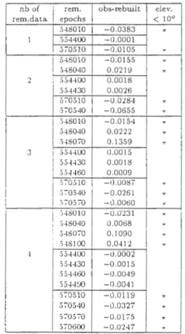
Ta-ble 1: we removed one to four data points at three different epochs in the satellite pass corresponding to different elevation angles and we tried to rebuild

these removed values.

The fi.rst and the last epochs choosen

(.548

010

and

.)ï0510l correspond to an elevation angle below 10

degrees. the other d~ta points are above

30

degrees.

It was important to consider low elevation angles in

our 1vork to study the limitations of this method as the si~nal to noise ratio of the GPS signal is much lower for low elevations. Consequently. the

mea-surement noise is higher and the number of cycle

slips is more important. In addition. the multipath

effect is also more frequent in the case of low P.!eva-tion an~les. Table

1 shows that the accuracy

of the restored 1·alue:; is oï the orcier of the measurement noise. The accuracy of the recovered data depends

of course on the number of '!ost' data.

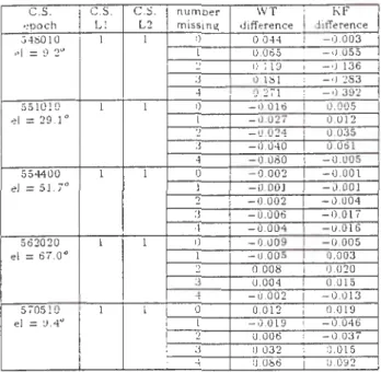
Table :; ~ives the results of the second and t.hird tests ·.,·here we introduced a jurnp of 1 cycle on L1 and 1 ,:.-de on L~( l. 1 ). Before this jump, a gap of ze:r0 !ù four data points was simulated. Again

the accuracy

o

i

the computed jump is of the ordcr

of the measurement noise. The rcsults obtained by

I..:alm::m filtE'ring and the wavdet transform arc of

the same orcier. Obviously, the computed jumps are

worse in the case of a low elevation angle. Other values th an ( 1.1) for the cycle slip give the sa me

results.

Table 1 and Table 2 display results for 4 missing

data. :; o test has be en made for !ar ger gaps, but it is obvious that the more the measurement noise is important, the more it will be difficult to recover

data and evaluate cycle slips after a large gap.

nb of rem. obs-rebuilt elev.

rem.data epochs

<

100 5-!8010 -0.0383 _"' 1 554400 -0.0001 570510 -0.0105 _" 5-!8010 -0.0155

*

5-!8040 0.0219

*

2 554400 0.0018 55-1430 0.0026 5 70510 -0.0284

*

570540 -0.0655

*

1 548010 -0.0154

*

548040 0.0222 _"' .)480ï0 0.1359 _"' 3 554400 0.0015 55-!430 0.0018 55-!460 0.0009 .570510 -0.008ï _"' 570540 -0.0261 _"' 1 .)705ï0 -0.0060 'K 1 548010 -0.0231 1 " 548040 0.0068 _"' 5480ï0 0.1090 _" .548100 0.0412 _" ·1 554400 -0.0002 .)5.J.J30 -0.0015 .)5.J.J60 -0.0049 S5H90 -0.0041 1 .570510 -0.0119 _"' 1 570540 -0.0327 _"' S705ï0 -0.01 ï5 "' .)70600 -0.024ï _"'

Table 1: Reconstruction of removed observations using the modulus of the wavelet transform.

Col-umn 1 gives the number of removed data points.

Column 2. the epochs (in GPS time) of remm·ed observations and Column 3. the differences between

the observed and the reconstructed values in cycles.

:\

*

appears in Column 4 when the removed data

correspond to an elevation lower than

10

degrees.

.-c.s. c.s. c.s. number WT KF

~po ch LI L2 missi ng difference difference

j48010 1 1 tl 0.044 -0.003 el = 9.:?~ 1 0.065 1 0.055 ~ 0 119 1 - 0.136 :J 0.181 0.283 4 0.2ï1 1 - 1) 392 551010 1 1 0 -0.016 0.005 el = 29.1" 1 -0.02ï 0.012 :! 0.024 0.035 3 -0.040 0.061 4 -0.080 0.005 554400 1 1 0 -0.002 - 0.001 el = 51. ï" 1 -0.001 -0.001 2 -0.002 - 0.004 :J 0.006 0.01 Î 4 -0.004 -0.016 562020 1 1 0 -0.009 - 0.005 el = 6ï.O" 1 0.005 0.003 2 0.008 0.020 :J 0.004 0.015 4 - 0.002 1 - 0.013 5 ï051 0 1 1 0 0.012 1 0.019 el = 9.4" 1 .).0 19 ₁ 0.046 2 0.006 1 - 0.03ï :.l 0.032 1 0.015 4 0.086 0.092

Table 2: Evaluation of known jumps. Column 1 gives the epoch (in

G

P

S

seconds) at which a cycle slip has been added and the elevation

(e

l

)

of the satellite at this epoch: Column 2 and Column 3 give (in cycles) the jumps added respectively on Ll and L2; Column 4 indicates the number of missing data points before the jump; Column 5 gives (in cycles) the difference between the jump added and the jump detected by the wavelet transform on the

P

P

combi11ation: Column 6 gives (in cycles) the results of the sa me test for the Kalman fil ter.

FILE S. V.# epoch of '!lev gap Wavelet Transt'orm

1

Kalman tilter

il

·1ata cycle slip PC1 PC:! 1 pp PC1 PC:! pp

1471.1 21 380310 gù ~0 6 - 17 1 0.009 1 2 0 -0.315 1 1471.:? 2 ·113790 12v 60 - 1 -2 1 [) 07. 1 -4 - 1 -ù 055

.

1 1481 2 1 l ï 446880 12° (10 1 13 0 1 -O.Oï6 1 1 -3 - 0.126

Il

1491.1 1 19 537030 13u 60 1 - 3 2 1 - 0.036 0 0 -0.036

I

l

26 530760 10° 90 -7 15 0.065 - 3 -2 -0.248 31 537510 sa ~0 -7 0 0.025 0 0 0.096 1491.2 13 522630 24° 120 1 1 - 0.041 1 0 -0.039 1 14 522720 19° 210 3 - 1 0.073 -3 - 1 0.048 19 522660 37° 150 2 2 - 0.044 1 0 0.065 !1 ~:? 522660 10° 60 0 0 - 0.036 3 l -0.021 24 '>22660 45° 150 0 -1 -0.012 -3 -2 0.062 29 .';22660 39° 150 0 0 0.014 0 0 -0 006

i

l

Table

:3

:

Comparison of calculated residuals and 'real' residuals. [n the tirst part of Table

:3.

Column 1 givcs the name of the data file. Column 2. the satellite number. Column 3. the epoch of the cycle slip (in

c_

;p

s

seconds). Column -+.the satellite elevil.tion. and Column .}. the duration (in seconds) of the gap in

the Jata. The ~econd part of this Table display,; the rPsults obtained by the wavelet transform tin cycles!. I t giws the difference het ween the ., real" residual compll ted wi th the value of the cycle slip fou nd by the double differ~nce ,;oftware and the residual computed by the wavelet transform ( l) for the si~nal

PC

₁ (Colurnn 1). (:.!l fr;r the signal

PC

2 (Colurnn :.!). and (:3) the

PP

combination (Column :)). The thire!

part oit he Tablè ron tains the sa me information as part :2 conce rn in:?; the resul ts of the l(;dman til tt'r tin cycles'!.

3.3

Real

cycle

slips

in GPS

data

ln 1993, the Royal Observatory of Belgium' (ROB)

has purchased four Turbo Rogue GPS receivers in

orcier to participate in the

IGS

network and as

sup-port to deploy the national G PS geodetic network.

This new receiver type is characterized by a very

law measurement noise.

The results of the previous paragraph de

mon-strate clearly th at the quality of the signal will play

a very important role in the cycle slip correction.

In may 1993, two of these four receivers were

con-tinuously operating during three days on a 83

me-ters baseline in the park of the Observatory. The

sampling interval was 30 seconds and the elevation mask 4 degrees.

First the cycle slips 'having no interest' were eli

m-inated. For example, if a satellite pass begins with

three data points followed by a gap of 2 minutes and

finally uninterrupted measurements during severa!

hours. the first three measurements are eliminated.

Then a cycle slip repairing was attempted on the six

data files using the wavelet transform. the Kalman

filter and double differences computed by the se

lf-written ROB-GPS software. Table 3 compares the

differences between the first residuals (Observed

-Predicted) on ?Cl. PC2 and PP computed by the

wavelet transform and the Kalman filter and the

'correct' residuals computed with the value of the cycle slip found using the double differences. From

a general point of vue. the Kalman filter gives

bet-ter results in the ?Ci modelisation: a Kalman filter with good a-priori values is ·weil suited to describe

a noisy signal.

On the other hand. the wavelet transform ob

-tains better

PP

residuals. The two methods are

thus very complementary.

lution was tried: the Kalman filter was applied on

the data in the two directions (from the beginning

to the end of file and from the end to the beginning)

gi ving two res id uals (one in each direction) for

ev-ery test quantity

(PC

1 ,

PC

2 ,

PP).

The mean

PC

residual was computed when encountering a cycle

slip. This supplementary step was not sufficient to

guarantee a correct computation of the PP res

id-ual. Then an attempt was made to madel the error

in the PP value predicted by Kalman filtering in

the two directions giving two more residuals.

The mean of these four PP residuals gave a value

precise enough to obtain an unambiguous value for

the cycle slip.

In the case of the wavelet transform method.

the problem is solved as follows: the first cycle slip evaluation is used to correct the signais PC1 , PC2

and PP giving the corrected signais ?Cl, PC~ and

P P

1_{. The wavelet transform is then recomputed on} the ionospheric free combination PP1

.

A new residual on

P

?

1 _{is found and is due to the} error on the first evaluation of the cycle slips on

PC₁ and PC2 . The first differences around the c

y-cle slip in the corrected signais PCf and PC~ are

used to find the complementary correction to apply on PC/ and PCi. This complementary correction

has to correspond with the new residual found on

ppl

As a last verification. the wavelet transform is r

e-computed on the three signais : PC?. PCi and

P P2 . If there remains a jump, a new iteration is

necessary.

\\"hen these supplementary steps 1\·ere

accom-pished. both methods gave the correct cycle 5lip

value.

These comments are less true for the file 1-191.2 but

4

_{Discussion and Conclusions}

in this case, the cycle slips occur above 19° of ele

-vation when the pseudorange noise is much lower. To be sure to obtain a unique solution for the cycle

slip, the accuracy of the

PC

residual has to be in-duded in a

(-:3. 3) cycles

interval around the correct cycle slip. In this case. the predicted

PP

residu al

has to be in a [ -·~ .1-1. 0 .1·!] interval around the co r-rect PP resiJual provided that a 1.1 or -l.-1 cycle slip gi\·es a -0.28 or 0.28 jump in

PP

Table

:3

shows that none of the two methods ran

rcalize these conditions in a hundred percent of the

cases. This result •'xplains why further de\·elopmem

w;ts necessary.

ln the case of the Kalman filter t.he following

so-The aim of this paper was to demonstrate that the

wavelet transform can be used to remon' cycle slips

in GPS measurements.

We showed th at the method can ev al ua te

mi5s-ing data and correct simulated cycle 5iips even if

they occur after a gap in the data. The accuracie5

achieved by the 1\.a\·elet transform and the 1\alman

filter ;ue of the same arder.

The ad van tage of the wawlet transform method

lies in the fact that the filter is easy to implement.

lt is very precise in the time location 0f a cycle

;;lip and a response on

;3

poims rnakes the detection

The disadvantages of this method are 1) that the

filter is a non-adaptative, one. 2) a signal with a lot

of noise can be seen as successive jumps.

The use of a Kalman tilter requires a set of ini-tial conditions: state vector, covariance matrix of

the observations, state-transition noise matrix. The Kalman filter is very sensitive to these a priori val-ues. Ideally, they should be adapted to the

differ-ent situations that can be encountered: these values vary in function of the receiver type, the site (mul-tipath), the ionospheric conditions, ...

However, a sui table choice of these initial conditions will give a powerful tool to study a signal deterio-rated by noise.

The wavelet transform does not need any a

pri-ori ·value, is very simple to implement but does not

give as good results as the Kalman filter on noisy

signais (i.e. the

PC;

combination) but better

re-sults on the

PP

combination.

As presented in the previous section. The use

of supplementary developments after obtaining the first residuals is necessary to find the exact cycle slip with each of the two methods.

As a consequence, the two mathematically inde-pendent methods seem to be very complementary and should be used together to give mutual confir

-mation of the computed cycle slips.

5

Acknowledgments

VVe should like to thank Prof. J-P. Antoine to have

introduced us to the theory of wavelets. We are also grateful to P. Pâquet, B. Ducarme and C.Bruyninx for useful comments. K.Degryse and \'.Dehant for

their help in the English translation.

References

[1.]1\'ave/ets. Time-Frequency Melhods and Phase

Spa ct ( Proc . .\[ arsezlle. Dec. 1987),

.J .<'.!. Combes. A. Grassmann. Ph. Tchamitchian

(eus.1. Berlin: Springer-Verlag, 1089. :2d eu., 1990.

A. Arnéodo. G. Grasse au, ~1. !Iolschneider. Wanlet anall)sis of multzfracials.

Phys. Rev. Lett. 131. pp. :2281-2284. n1~8. L. Ba.;;tos. H. Landau.

Fixznq cycle slips zn dual frcquency kznonalic GPS

rzpplzcatzons uszng !l'a/man filtering,

~Ianuscripta Geodetica, 13, pp. 249-256, 1988.

A. Bijaoui,

r.-1.

Giudicelli,

Optimal image addition using the wavelet trans-form. Experimental Astronomy, 1, pp. 347-363, 1991. CH. K. Chui, An Introduction ta Wavelets, Academie Press, 264 pp., 1992. I. Daubechies,

Ten Lectures on Wavelels,

SIAM

.

357 pp., 1992. I. Daubechies,

Orthonormal bases of wavelets wilh finite support -Connection with discrete fillers,

in

[1.],

pp. 38-67.

~- Delprat, B. Escudié.

R. Kronland-:\lartinet, Ph. Torrésani.

Ph. Guillemain.

Tchamitchian. B. Asymptolic wavelet and Gabor analysis: Extractzo1z

of Inslantaneous frequencies,

IEEE transactions on Information Theory, 38. 2.

pp.644-664, 1992.

H.J. Eueler and C. Goad,

On optimal filtering of GPS dual frequency

obser-eatzons wilhoul using arbil information.

Bulletin géodésique.

6.5

pp. 130-143. 1991. A. Grassmann. J. ~!arlet, T. PauL

Transforms associated la square integrable group representation !. Gr: nera/ results.

J. l'v! ath. Phys .. 26. pp. 2473-2-!79. 198.).

A. Grassmann. Ph. Guillemain.

R.

Kronland-~lartinet.

Arête associée à la transformée en ondelettes de s ig-naux présentant des singularités isolées.

Proceedings of the International conference on

·wavelets and .\pplications'. Toulouse. 1992. to be published.

P. Guillemain. R. Kronland-~lartinet. B. :VIartens.

"A.pplication de la transformée en ondelettes en

spectroscopie R.\fN''.

rapport CNRS-DIA (~larseille), Noll2. 1989.

Ph. Guillemain,

R

.

Kronland-.Martinet,

Parameters estimation through continuous wavelet

transform for synthesis of audio-sounds,

an audio engineering society, prepint 1991.

M. Holschneider, R. Kronland-Martinet,

J

.

Morlet, Ph. Tchamitchian,

A real-lime algorithm for signal analysis with the

help of the wavelet lransform,

in [1.], pp. 286-297.

R.W. King, EG :\[asters, C.Rizos, A.Stolz and

J

.Collins,

Surveying with Global Positioning System,

Dümmler. Bonn. 1987.

H. Landau.

Preczse J.:inematic CPS positioning: Experiences on

a Land Vehicule using TI ~ 100 receivers and soft

-ware.

Bulletin géodésique.

6

:3.

pp. 8.)-96, 1989. H. Li ch tenegger. B. Hoffmann- Wellenhof. CPS data preprocessing for cycle slip detection.

Paper presented at the 125th Anniversary General

:VIeeting of !AG. Edinburgh. 1989.

B. ;\[artens,

"':lpplica

lion

de

/"analyse

en

ondelettes à la R.l!X··.

:VIémoire de Licence. UCL. Louvain-la-~euve, 1989.

Y. \leyer.

"'Onde/elles : Algorzthmes el applications··

Ed. Armand Colin. 184 pp .. 1992. E. Slezak. A. Bijaoui. G. ;\lars.

!dentzficalzon of structures from galaxy counts: use

vf tht 1cavelet transform,

:\:itron. Astrophys .. '227. pp. :301-:nô. 1990. !3. Torrésani.

Un logzczel d'anailjse en ondelettes par l"agonthmr 11 trous.

Rapport no:). C.:ntrc de Phy~ique théorique C:\R:) -Luminy. 1088.