A Complexity Approach for Core-Selecting Exchange under
Conditionally Lexicographic Preferences
Etsushi Fujita [email protected]
Kyushu University,
Motooka 744, Fukuoka, Japan
Julien Lesca [email protected]
Universit´e Paris Dauphine, PSL Research University, CNRS, LAMSADE, Paris, France
Akihisa Sonoda [email protected]
Kyushu University,
Motooka 744, Fukuoka, Japan
Taiki Todo [email protected]
Kyushu University,
Motooka 744, Fukuoka, Japan
Makoto Yokoo [email protected]
Kyushu University,
Motooka 744, Fukuoka, Japan
Abstract
Core-selection is a crucial property of rules in the literature of resource allocation. It is also desirable, from the perspective of mechanism design, to address the incentive of agents to cheat by misreporting their preferences. This paper investigates the exchange problem where (i) each agent is initially endowed with (possibly multiple) indivisible goods, (ii) agents’ preferences are assumed to be conditionally lexicographic, and (iii) side payments are prohibited. We propose an exchange rule called augmented top-trading-cycles (ATTC), based on the original TTC procedure. We first show that ATTC is core-selecting and runs in polynomial time with respect to the number of goods. We then show that finding a beneficial misreport under ATTC is NP-hard. We finally clarify relationship of misreporting with splitting and hiding, two different types of manipulations, under ATTC.
1. Introduction
Designing rules/mechanisms that achieve desirable properties is a central research topic in the literature of mechanism design and social choice theory. An assignment problem is defined by a set of indivisible goods and a set of agents, and the purpose is to compute an assignment of goods to agents such that no good is assigned more than once. Such an assignment should prescribe a socially desirable outcome in the sense that the assignment should reflect the preferences of the agents over goods. In this paper we study the exchange problems which is a particular assignment problem with following properties: (i) each agent is initially endowed with a set of indivisible goods, (ii) each agent has a strict ordinal preference relation (shortly, a preference) over the set of possible bundles of goods, and (iii) compensation using monetary transfers is prohibited. The
ex-change problem has many real applications, such as on-campus university housing markets (Chen & S¨onmez, 2002) and nation-wide kidney exchanges (Roth, S¨onmez, & ¨Unver, 2004).
Core-selection is one of the most well-studied properties that exchange rules are expected to achieve. An exchange rule is said to be core-selecting if no group of agents has an incentive to make a cartel and trade their goods among themselves. By definition, core-selecting rules encourage agents to participate in the rules (i.e., implies individual rationality) and result in a Pareto efficient trade of goods, which in a sense is a socially optimal outcome. When each agent is assumed to be initially endowed with a single indivisible good, Gale’s Top-Trading-Cycles (TTC) procedure is known to be core-selecting (Shapley & Scarf, 1974; Roth & Postlewaite, 1977).
Another common requirement is strategy-proofness, which requires that each agent has no incentive to misreport her preference. To be more precise, for each agent, submitting her true preference to the exchange rule is a dominant strategy. This is a quite strong requirement for agents’ incentives. Actually, S¨onmez (1999) showed that, when there is at least one agent who initially owns more than one good and the agents’ preferences over bundles of goods are strict, as in our exchange problems, there exists no rule that is simultaneously strategy-proof and core-selecting in general.
In the wake of this impossibility, we tackle the incentive issue from the perspective of com-putational complexity. The idea is as follows: even if an agent is selfish and hopes to benefit by misreporting, if finding a beneficial misreport is hard, e.g., it requires to solve an NP-hard prob-lem, and its power of computation is limited, then it will refrain from doing such a manipulation. Under this assumption, in a sense, the NP-hardness of finding a beneficial preference misreport guarantees that agents do not have strong incentive to misreport their preferences. Such a com-plexity approach for agents’ incentives has attracted much attention from computer scientists, especially in the literature of computational social choice (Bartholdi, Tovey, & Trick, 1989; Pini, Rossi, Venable, & Walsh, 2011).
In the exchange problem, agents have preferences over bundles of goods. Describing prefer-ences by an exhaustive ordering of the bundles may be infeasible whenever the number of goods is too large. Indeed, the number of bundles growths exponentially with the number of goods. There-fore, compact representations are worth considering for representing preferences of the agents in our exchange problem. The lexicographic preferences are a well studied restriction over the pref-erence domain which allows a compact representation of the prefpref-erences (Saban & Sethuraman, 2014; Todo, Sun, & Yokoo, 2014; Aziz, Kalinowski, Walsh, & Xia, 2016). Indeed, under this restric-tion the preferences over bundles can be fully described by an ordering over goods. Informally speaking, lexicographic preferences are defined as follows. In order to compare two bundles of goods, we start by comparing their most preferred goods. If the most preferred good in one bundle is preferred to the most preferred good in the other bundle then the former bundle is preferred to the later one. Otherwise, we compare the second most preferred goods of those bundles, and in case of equality, we compare the third most preferred goods, and so on. Let us consider an illustrative example with three goods: beef (B), cake (C) and white wine (W). Suppose that B is preferred to C which is preferred to W. In lexicographic preferences model, the preferences over bundle is {B, C, W} {B, C} {B, W} {B} {C, W} {C} {W}, where means that the left part is strictly preferred to the right part.
The drawback of focusing on lexicographic preference domain is that such restriction seems too strong to reflect real preferences. In this paper we focus on a larger preference domain over bundles of goods, called conditionally lexicographic preferences, which was introduced by Booth,
Chevaleyre, Lang, Mengin, and Sombattheera (2010). Lexicographic preferences are a special case of conditionally lexicographic preferences. But the compact representation used to represent con-ditionally lexicographic preferences is richer in the sense that the ordering over goods may be conditional to the existence of some more preferred goods in the bundle. Let us change our exam-ple by replacing white wine with red wine (R). In that case, the preferences of an agent over the red wine and the cake may be different if she obtains the beef or not. For example, she may prefer R to Cif she has B, and otherwise she prefers C to R. In that case, the preferences over bundles would be the following: {B, C, R} {B, R} {B, C} {B} {C, R} {C} {R}. Note that such preferences are not lexicographic because C is once preferred to R and R is once preferred to C. Actually, the number of possible conditionally lexicographic preferences is exponentially larger than the number of possible lexicographic preferences (Booth et al., 2010).
In this paper, we propose an exchange rule called augmented top-trading-cycles (ATTC) proce-dure for the exchange problem. The proposed rule possesses nice properties in terms of quality of solutions and agents’ incentives. Concerning the quality of solutions, the ATTC procedure is core-selecting. For agents’ incentives, finding a beneficial misreport for a manipulator under the ATTC procedure is NP-hard. We also consider two different types of manipulations called split-ting and hiding, and clarify their relationship with preference misreporsplit-ting. We show that, for any given splitting/hiding manipulation, there exists a corresponding preference misreport that gives the same bundle of goods to the manipulator, and such a misreport can be computed in polynomial time.
The paper is organized as follows. In Section 2, we review several existing works and clarify the difference with our approach. In Section 3, we give the formal model of our exchange problems and define the conditionally lexicographic preferences. In Section 4, we define the ATTC procedure and illustrate its behavior by a simple example. In Section 5, we show that the ATTC procedure is core-selecting. In Section 6, we formalize the problem of finding a beneficial misreport under the ATTC procedure and show that it is NP-hard. In Section 7, we give the definitions of splitting and hiding manipulations, and present two algorithms to emulate these manipulations by misreporting preference. In Section 8, we conclude the paper and give some possible future research directions.
2. Related Works
The exchange model we deal with in this paper is a generalization of the well-studied housing mar-ket (Shapley & Scarf, 1974), where each agent initially owns a single house, agents’ preferences are strict, and monetary transfers are prohibited. In housing market literature, the TTC proce-dure is characterized by three properties: individual rationality, Pareto efficiency, and strategy-proofness (Ma, 1994). Moreover, it always chooses the unique core assignment (Roth & Postle-waite, 1977). Other properties have been considered in AI, e.g., fairness (Endriss, Maudet, Sadri, & Toni, 2006; Lesca & Perny, 2010; Lesca, Minoux, & Perny, 2013) and envy-freeness (Chevaleyre, Endriss, & Maudet, 2007; de Keijzer, Bouveret, Klos, & Zhang, 2009). Constraints on the set of possible allocations have also been considered, e.g., for exchanges over a social network (Gourv`es, Lesca, & Wilczynski, 2017). On the other hand, when at least one agent initially owns more than one house, as well as the impossibility result presented in the previous section advents, we can no longer guarantee the uniqueness of the core assignment (S¨onmez, 1999). Cechl´arov´a (2009) studied the exchange problem for more than one type of goods and show that deciding the nonemptyness
of the core is NP-hard even for two types of goods. Furthermore, Cechl´arov´a and Lacko (2012) studied the core property for the kidney exchange problem.
One common approach for going beyond such an impossibility result is to weaken one of the requirements. In the literature of exchange with multiple endowments, which is what we are dealing with in this paper, several strategy-proof rules have been developed by weakening the core-selecting property (P´apai, 2003, 2007; Todo et al., 2014). Various restriction over the pref-erence domain have also been considered in the literature, such as binary domain (Luo & Tang, 2015), asymmetric preferences (Sun, Hata, Todo, & Yokoo, 2015), and additive preferences (Sonoda, Fujita, Todo, & Yokoo, 2014; Aziz, Bir´o, Lang, Lesca, & Monnot, 2016).
Our approach maintains the core-selecting requirement, but weakens strategy-proofness by focusing on the computational hardness of beneficial manipulation. In various mechanism de-sign/social choice problems, many works consider the computational hardness of beneficial manip-ulation, such as voting (Bartholdi et al., 1989), two-sided matching (Teo, Sethuraman, & Tan, 2001; Pini et al., 2011) and sequential allocation (Aziz, Bouveret, Lang, & Mackenzie, 2017). Although it has been pointed out that such a computational complexity approach is not always sufficient as a barrier for agents’ incentives (Faliszewski, Hemaspaandra, & Hemaspaandra, 2010; Faliszewski & Procaccia, 2010), we believe that discussing complexity of misreporting in exchange problems is an important first step toward the development of useful exchange rules for self-interested agents in practice.
In this paper we also focus on the conditionally lexicographic preference domain. This re-striction leads to compact representations of the agents’ preferences, and makes sense whenever they are non compensatory (Gigerenzer & Goldstein, 1996). Thus such preferences have been well studied in the AI community and especially in elicitation (Booth et al., 2010) and voting (Conitzer & Xia, 2012; Lang, Mengin, & Xia, 2012). Responsive preferences are one of the most famous re-striction over the preference domain in matching theory. Such domain of preferences generalize both lexicographic and additive preferences. Informally, the requirement for a preference to be responsive is that, for a given bundle of goods, the marginal contribution of an additional good only depends on the ordering over goods. Note that, according to the illustrative example provided earlier, conditionally lexicographic preferences may not be responsive.
Similar exchange rules as ATTC procedure have been studied in recent papers (Sikdar, Adalı, & Xia, 2017, 2018). Sikdar et al. (2017) consider an exchange problem where goods are partitioned into types (car, house, and so on). Each agent has initially a single good of each type and receives at the end of the procedure a single good of each type. Therefore, preferences are over bundles of goods of same size with one good per type. Agents’ preferences are represented by CP-nets where vertices represent types. In short, CP-nets are an oriented graphs which represent condi-tional preferences over types. The preferences over the goods of a given type will depend on the other goods allocated whose types are parents in the graph of the type under consideration. In the paper, the CP-nets considered are lexicographic i.e., there exists a linear order over the types such that a type can be the ancestor of another one only if the first type precedes the second type in this linear order. This model somehow extends the one presented by Fujita et al. (2015), where agent’s preferences over the bundles of goods are lexicographic. However, the model of Sikdar et al. (2017) impose additional constraint on the admissible allocation (exactly one good per type) whereas such constraint does not appear in the paper of Fujita et al. (2015). Conditionally lexico-graphic preferences considered in this paper generalize the model studied by Sikdar et al. (2017) except that it does not allow indifferences. On the other hand, the model of preferences considered
by Sikdar et al. (2018) generalizes conditionally lexicographic preferences in order to allow indif-ferences. Sikdar, Adali, and Xia (2017, 2018) show that TTC-like procedures for these two models of preferences are core-selecting.
The effect of splitting manipulations has been studied in several algorithmic/economic en-vironments, such as scheduling (Moulin, 2008), voting (Conitzer, 2008; Todo, Iwasaki, & Yokoo, 2011), combinatorial auctions (Yokoo, Sakurai, & Matsubara, 2004), two-sided matching (Todo & Conitzer, 2013; Afacan, 2014), and coalitional games (Aziz, Bachrach, Elkind, & Paterson, 2011; Yokoo, Conitzer, Sandholm, Ohta, & Iwasaki, 2005; Ohta, Conitzer, Satoh, Iwasaki, & Yokoo, 2008), some of which are also known as false-name manipulations. Especially for the case of exchange problem, a class of exchange rules resistant to splitting manipulations, as well as to another class of manipulations called hiding (Atlamaz & Klaus, 2007), has been proposed by Todo et al. (2014), while they do not satisfy the core-selecting property.
3. Preliminaries
In this section we provide the formal definition for the exchange problem with multiple indivisible goods studied in this paper as well as several properties of exchange rules that have been discussed in the literature.
3.1 Notation
We consider set of agents N = {1, . . . , n} and finite set of heterogeneous indivisible goods K of size m. An assignment x = (x1, . . . , xn) is a partition of K into n subsets, where xi is the bundle of goods assigned to agent i under assignment x. We denote by X the set of all possible assignments.
The assignment of the goods to the agents is made based on their preferences, which are or-ders/rankings over bundles of goods. In this paper we focus on the domain of conditionally lexico-graphic preferences, in which a preferences over the bundles of goods are modeled by lexicolexico-graphic preference trees (or LP-trees).
Definition 1(LP-tree). An LP-tree over K is a rooted tree such that • every vertex v is labeled with good g(v) belonging to K
• every good appears once, and only once, on any path from the root to a leaf
• every non-leaf vertex v has either one outgoing edge labeled by g(v) ∨ g(v), or two outgoing edges labeled by g(v) and g(v), respectively.
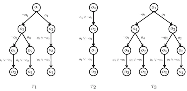
Figure 1 provides three examples of LP-trees over K = {o1, o2, o3, o4}. Let L be the set of all possible LP-trees over K. For any vertex v of an LP-tree, let a(v) be the set of goods labeling the ancestors of v, i.e. the vertices on the path from the root to v. For example, in τ1described in Figure 1, if we define v as the leftmost vertex with label o4then a(v) = {o1, o3}. An LP-tree τ represents a preference over bundles in a graphical manner. In order to evaluate a bundle A ⊆ K, we follow the directed path starting from the root, ending at one of the leaf and containing only edges consistent with A, i.e. for each vertex v visited by this directed path, an edge consistent with A would be labeled by either g(v) or g(v) ∨ g(v) if g(v) ∈ A, and by either g(v) or g(v) ∨ g(v) otherwise. Note that such a path is unique. Let τ(A) denote such a path. For example, τ1({o1, o2})is the path
Figure 1: Three examples of LP-trees
from the root that reaches the rightmost leaf, and τ3({o2, o3})is the path that reaches the leftmost leaf. In order to compare two bundles A and B, with A 6= B, we consider the first vertex v in the sequence of vertices visited by both τ(A) and τ(B) and such that g(v) belongs to exactly one of the two bundles. Let τ(A, B) denote such vertex. For example, τ1({o2, o3}, {o2, o4})is the leftmost vertex labeled by o3 and with two children in τ1, and τ3({o1, o2, o3}, {o1, o3})is the rightmost vertex labeled by o2and with two children in τ3. More formally, τ(A, B) is the unique vertex that is visited by both τ(A) and τ(B) and such that a(τ(A, B)) ⊆ A ⊕ B and g(τ(A, B)) 6∈ A ⊕ B, where A ⊕ B = {o ∈ K | o ∈ A ⇔ o ∈ B}. Preferences associated with LP-trees are defined as follows:
Definition 2. For a given LP-tree τ, let τdenote the preference over bundles such that, for any two bundles A, B ⊆ K, A τ Biff both g(τ(A, B)) ∈ A and g(τ(A, B)) 6∈ B hold.
For example, considering the LP-tree τ1 of Figure 1, we have {o2, o3} τ1 {o2, o4}because g(τ1({o2, o3}, {o2, o4})) = o3 and o3belongs to {o2, o3}but not to {o2, o4}. Note that both τ1 and τ3 are not responsive, and τ2 is lexicographic because τ2 is a path. In order to simplify notation, we denote by %τthe preference such that for any A, B ⊆ K, A %τ Biff either A τ B or A = B holds.
In the rest of this paper, we assume that agent preferences are conditionally lexicographic and that the preference of each agent is represented by an LP-tree. Using this notation, we de-fine an exchange problem (e, τ ) by an initial endowment e = (e1, . . . , en) ∈ X and a pro-file τ = (τ1, . . . , τn) ∈ Ln of LP-trees, where τi denotes the LP-tree that models the prefer-ence of agent i. For any i ∈ N and any τ0
i ∈ L, we denote by (τi0, τ−i)the preference profile (τ1, . . . , τi−1, τi0, τi+1, . . . , τn). Furthermore, we denote by δ(o) the owner of o in e.
Example 1. Consider the set of goods K = {o1, o2, o3, o4}, the set of agents N = {1, 2, 3}, and the initial endowments e such that e1 = {o1, o4}, e2 = {o2}, and e3 = {o3}. The LP-trees τ = (τ1, τ2, τ3)presented in Figure 1 describe the conditionally lexicographic preferences of agents 1, 2 and 3, respectively. The pair (e, τ ) defines an exchange problem.
3.2 Exchange Rules and Properties
An exchange rule is a function ϕ : X ×Ln→ Xthat maps any exchange problem to an assignment. Let ϕi(e, τ )denote the bundle assigned to agent i under assignment ϕ(e, τ ). In this section, we provide the formal definitions of three properties achievable by an exchange rule, namely individual rationality, Pareto efficiency, and core selection. These properties have traditionally been considered as desiderata in the literature of social choice and mechanism design.
Definition 3(Individual Rationality). For a given exchange problem (e, τ ), an assignment x ∈ X is individually rational if xi %τi eiholds for any agent i. An exchange rule ϕ is individually rational (IR) if for any exchange problem (e, τ ), ϕ(e, τ ) is individually rational.
In other words, for each agent, as long as she truthfully reports her preference, she is never worse off by participating in an IR exchange rule. Under such an exchange rule, every agent is incentivized to participate.
Definition 4(Pareto Efficiency). For a given exchange problem (e, τ ), an assignment x ∈ X is Pareto dominated by another y ∈ X if (i) yi %τi xi holds for every i ∈ N, and (ii) yj τj xj holds for some j ∈ N. An assignment is Pareto efficient if it is not Pareto dominated by any other assignment. An exchange rule ϕ is Pareto efficient (PE) if for any exchange problem (e, τ ), ϕ(e, τ ) is Pareto efficient.
When an assignment x is Pareto dominated by another assignment y, choosing x is sub-optimal. Therefore, using a PE exchange rule is socially optimal, in the sense that it never chooses such sub-optimal assignment.
Definition 5(Core Selection). For a given exchange problem (e, τ ), a coalition T ⊆ N of agents blocks an assignment x ∈ X if there exists another assignment y ∈ X such that (i) yi ⊆ S`∈Te` for every i ∈ T , (ii) yi %τi xi for every i ∈ T , and (iii) yj τj xj for some j ∈ T . The core C(e, τ ) is the set of assignments that are not blocked by any coalition. An exchange rule ϕ is core-selecting (CS) if for any exchange problem (e, τ ), ϕ(e, τ ) ∈ C(e, τ ) holds.
Condition (i) means that a blocking coalition is restricted to the goods initially owned by the agents in this coalition. Conditions (ii) and (iii) means that, assignment y Pareto dominates x when we only consider the preferences of the agents belonging to the blocking coalition. Intuitively, the existence of a coalition T of agents that blocks an assignment means that they jointly have incentives to form a cartel and get higher utility by leaving behind the set N \ T of all the other agents. When an exchange rule is CS, one can expect that all agents participate without forming any such cartel. In this sense, CS can be regarded as a refinement of IR to any possible coalition of agents. Furthermore, by setting T = N, the definition coincides with PE. Thus, if an exchange rule is CS, it is also PE and IR.
Example 2. Consider the exchange problem of Example 1. Assignment x1= ({o1, o4}, {o2}, {o3}) = eis obviously individually rational but it is Pareto dominated by x2= ({o1, o3}, {o2}, {o4}). On the other hand, x3 = ({o
1, o2}, {o3}, {o4})is Pareto efficient but not individually rational, since agent 2is worse off than his initial endowment. To see that, observe that τ2({o3}, {o2})is the unique vertex with label o2(see Figure 1), and g(τ2({o3}, {o2})) = o2belongs to {o2}but not to {o3}. The assign-ment x2is individually rational and Pareto efficient, but not in the core, because T = {1, 2} ⊂ N is a blocking coalition with the assignment x4 = ({o
1, o2}, {o4}, {o3}). Finally x4is in the core, and automatically individually rational and Pareto efficient.
Algorithm 1The Augmented Top-Trading-Cycles (ATTC) procedure Input: exchange problem (e, τ )
Output: assignment ϕ(e, τ )
1: t ← 1 2: Vt← K 3: for eachi ∈ N do 4: Xit−1← ∅ 5: end for 6: whileVt6= ∅ do
7: Et← ∅ .Construction of ATTC graph Gt= (Vt, Et)
8: for eacho ∈ Vtdo
9: Et← Et∪ {(o, g(τδ(o)(Xδ(o)t−1, Xδ(o)t−1∪ Vt)))}
10: end for
11: Wt← ∅
12: for eachi ∈ N do .Assignment of goods to agents in each cycle of Gt
13: ifexists o ∈ Vt∩ eivisited by some cycle C in Gtthen
14: Let f denote the successor of o in C
15: else 16: Xt i ← Xit−1∪ {f } 17: Wt← Wt∪ {o} 18: end if 19: end for
20: Vt+1← Vt\ Wt .Removal from Gt+1of assigned goods
21: t ← t + 1
22: end while
23: return(Xit−1)i∈N
Combining the fact that CS property implies both IR and PE properties with the general im-possibility result by S¨onmez (1999), or more straightforwardly with the non-existence of an ex-change rule that is IR, PE, and strategy-proof under the lexicographic preference domain by Todo et al. (2014), we can easily conclude that there exists no exchange rule that is CS and strategy-proof, even under the conditionally lexicographic preference domain. Our purpose in this paper is therefore to design an exchange rule that is CS and computationally hard to manipulate, while it is inevitably not strategy-proof.
4. Augmented Top-Trading-Cycles Rule
In this section we propose a new exchange rule, called augmented top-trading-cycles (ATTC), which is inspired by, and indeed is a natural extension of, the well-known Gale’s Top-Trading-Cycle (TTC) procedure. Informally, TTC is a stepwise algorithm simulating a market place, where at each step, the remaining agents point to the most preferred remaining good according to their preferences. The agents which are part of a cycle during a step of the algorithm are assigned to the good they are pointing to and leave the market. ATTC generalizes TTC to exchange problems where agents may have more than one good by dividing each agent into several atomic agents, each
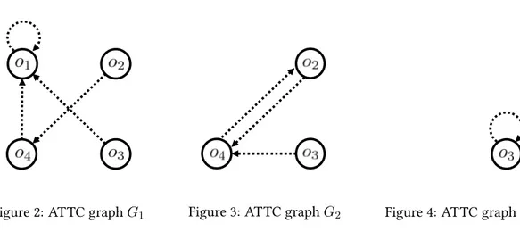
Figure 2: ATTC graph G1 Figure 3: ATTC graph G2 Figure 4: ATTC graph G3
of which is assigned exactly one good from the original agents’ endowments. Then the standard TTC procedure is applied to these atomic agents. Obviously, when each agent is initially endowed with a single good, ATTC results in an assignment identical to the one returned by TTC.
In order to apply the TTC procedure to conditionally lexicographic preferences over bundles, we need to know at each step which good is the best to complete the bundle already assigned to one agent. Assume that Xt
i is the bundle of goods assigned to agent i during the first t steps, and Vt+1are the remaining goods in the market. The best good to complete Xit, according to the preference of agent i, should be the good o labeling the first vertex on the path τi(Xit)with a label in Vt+1. For example, assume that Vt+1= {o2, o3, o4}and X1t= {o1}. In that case, the sequence of labels on the path τ1({o1})is (o1, o2, o3, o4). Therefore, o2is the best good to complete Xit. To see why, one could compare {o1, o2}and {o1, o3, o4}according to agent 1 preference τ1, and see that {o1, o2}is preferred to {o1, o3, o4}. The vertex we are referring to i.e., the first vertex on the path τi(Xit)with a label in Vt+1, is the vertex τi(Xit, Xit∪ Vt+1). Algorithm 1 provides a formal description of ATTC.
In the following, we will refer to the graph Gtas the ATTC graph during step t. Furthermore, function ϕ will denote the ATTC procedure as described in Algorithm 1. Note that at any step t in the procedure, the ATTC graph Gtcontains at least one cycle, and such a cycle contains at least one good, from the characterization of the original TTC procedure. Therefore it is clear that the running-time of ATTC is polynomial with respect to m, the number of goods.
Example 3. Consider once again the exchange problem presented in Example 1, where δ(o1) = 1, δ(o2) = 2, δ(o3) = 3, and δ(o4) = 1. At the beginning of ATTC, agent 1 is divided into two atomic agents, say 10and 100, each of which has the same preference as agent 1, and o
1and o4are the initial endowments of 10and 100, respectively. Furthermore, initially X0
1 = X20 = X30 = ∅. Then the original TTC is applied for the market with four atomic agents 10, 100, 2 and 3 with initial endowment {o
1}, {o4}, {o2}and {o3}, respectively. The set V1of vertices of the ATTC graph G1is {o1, o2, o3, o4}, and the arrows of E1 are (o1, o1), (o4, o1), (o3, o1), and (o2, o4). The graph G1 is illustrated in Figure 2. During step 1, vertex o1 is the only vertex included in a cycle, and thus the good o1is assigned to agent δ(o1) = 1. Furthermore, after this step W1 = {o1}, X11 = {o1}and X21 = X31 = ∅. After the removal of W1, the set of vertices of the ATTC graph G2 is V2 = {o2, o3, o4}, and the arrows are (o2, o4), (o3, o4), and (o4, o2). The graph G2 is illustrated in Figure 3. During step 2, there is a cycle containing the vertices o2and o4. Therefore, the good o2is assigned to agent δ(o4) = 1and the
good o4is assigned to agent δ(o2) = 2. Furthermore, after this step W2 = {o2, o4}, X12 = {o1, o2}, X2
2 = {o4} and X32 = ∅. After the removal of W2, the set of vertices of the ATTC graph G3 is V3 = {o3}, and the unique arrow is (o3, o3). The graph G3 is illustrated in Figure 4. Finally during step 3, the good o3 is assigned to agent δ(o3) = 3. Furthermore, after this step W3 = {o3}, X3
1 = {o1, o2}, X23 = {o4}and X33 = {o3}. After the removal of W3, V4 = ∅and the algorithm terminates. The final assignment is then x = ({o1, o2}, {o4}, {o3}), which is in the core as we observed in Example 1.
5. Core Selection
We observed, from Example 3, that there is at least one exchange problem for which ATTC returns an assignment in the core. In this section we generalize this observation and show that ATTC inherits the CS property from the original TTC procedure under the conditionally lexicographic preference domain.
In order to introduce this result, we first show that the comparison of two bundles, A and B, with A 6= B, through a conditionally lexicographic preference τ only depends on the goods belonging to a(τ(A, B)) ∪ g(τ(A, B)) i.e., the labels of the vertices visited by both path τ(A) and path τ(B) before attaining vertex τ(A, B). Intuitively, we need to show that if C and D are bundles which differ from A and B, respectively, only over the goods outside of a(τ(A, B)) ∪ g(τ(A, B)) then τ(A, B) and τ(C, D) should refer to the same vertex of τ. Therefore A τ B iff C τ D according to Definition 2.
Lemma 1. For any τ ∈ L, any A, B ⊆ K and any C, D ⊆ K, with A 6= B and C 6= D, if a(τ (A, B)) ∪ g(τ (A, B)) ⊆ (A ⊕ C) ∩ (B ⊕ D)i.e., o ∈ A iff o ∈ C and o ∈ B iff o ∈ D for any good o ∈ a(τ(A, B)) ∪ g(τ(A, B)), then τ(A, B) = τ(C, D).
Proof. By definition of τ(A, B), we know that for any o ∈ a(τ(A, B)) we have o ∈ A ⇔ o ∈ B, and this implies that o ∈ C ⇔ o ∈ D since o ∈ A ⇔ o ∈ C and o ∈ B ⇔ o ∈ D hold. Therefore, a(τ (A, B)) ⊆ C ⊕ Dholds, and τ(A, B) is visited by both τ(C) and τ(D).
On the other hand, we know that g(τ(A, B)) ∈ A ⇔ g(τ(A, B)) /∈ B. Hence g(τ(A, B)) ∈ C ⇔ g(τ (A, B)) /∈ D, since g(τ(A, B)) ∈ A ⇔ g(τ(A, B)) ∈ C and g(τ(A, B)) ∈ B ⇔ g(τ (A, B)) ∈ Dhold. This implies that g(τ(A, B)) /∈ C ⊕ D. Thus, vertex τ(A, B) is visited by both τ(C) and τ(D), and satisfies both a(τ(A, B)) ⊆ C ⊕ D and g(τ(A, B)) /∈ C ⊕ D. Therefore τ (C, D)coincides with vertex τ(A, B).
Note that during step t of ATTC, all the arrows, from the copies of agent i, are pointing to the same good labeling vertex τi(Xit−1, X
t−1
i ∪ Vt). As discussed earlier, this good is the best to complete the current bundle Xt−1
i of agent i. The next lemma shows that for any step t, the goods labeling the ancestors of τi(Xit−1, Xit−1∪ Vt)in τicannot belong to Vt.
Lemma 2. For any step t > 1 and for any agent i ∈ N, a(τi(Xit−1, X t−1
i ∪ Vt)) ⊆ K \ Vt. Proof. The bundle Xt−1
i of goods acquired by agent i after the first t − 1 steps of the procedure cannot contain any good belonging to Vt. Hence Xit−1 ⊆ K \ Vt. This implies that Xit−1⊕ (Xit−1∪ Vt) = K \ Vt. Furthermore, from the definition of τi(Xit−1, X
t−1
i ∪ Vt), we know that a(τi(Xit−1, Xit−1∪ Vt)) ⊆ Xit−1⊕ (Xit−1∪ Vt). Therefore, we have a(τi(Xit−1, Xit−1∪ Vt)) ⊆ K \ Vt.
Using these two lemmas, we can show that ATTC is core-selecting: Theorem 1. ATTC is CS.
Proof. For the sake of contradiction we assume that there exists an exchange problem (e, τ ) such that the assignment ϕ(e, τ ) = x, returned by ATTC, is blocked by a coalition T ⊆ N. Let y ∈ X be an assignment satisfying conditions (i), (ii), and (iii) described in Definition 5. Let Ut be the subset of agents that obtain a good during step t, let Tt= T ∩ Ut, and let xtibe the good obtained by agent i ∈ Ut during this step i.e., the unique good contained in Xit\ Xit−1. Note that such Xt
i \ Xit−1is a singleton because the arrows from all the goods belonging to agent i point to the same good during step t.
Here, for each step t in the procedure, consider the three following properties: • Ht
1: for any i ∈ Tt, xti∈ yiholds, • Ht
2: for any i ∈ Ttand any j ∈ N, xti ∈ ej ⇒ j ∈ T holds, • Ht
3: for any i ∈ Ttand any o ∈ a(τi(Xit−1, Xit−1∪ Vt)), o ∈ xi⇔ o ∈ yiholds. If we prove that Ht
1and H3tare true for any step t, then it will imply that for any i ∈ T , yi = xi holds, leading to a contradiction with conditions (iii) of Definition 5 i.e., yj τj xj holds for some j ∈ T. Therefore, to conclude the proof it suffices to show that Ht
1, H2t, and H3thold for any step t, where Ht
2is an important property to prove H3t. We will show them by mathematical induction with respect to t.
Base case (t = 1):We show that H1
1, H21, and H31hold. Let i be an arbitrary agent in T1. By definition of Algorithm 1, we know that x1
i labels the root of τi since Xi0 = ∅and V1 = K. If x1
i ∈ y/ 1, g(τi(xi, yi)) = x1i holds, which implies xi τi yi and contradicts the condition (ii) of Definition 5 i.e., yi %τi xiholds for any i ∈ T . Therefore, x
1
i ∈ y1 and thus H11 hold.
Let j ∈ U1be an arbitrary agent satisfying x1i ∈ ejfor some i ∈ T1. Assume by contradiction that j /∈ T . Therefore, x1
i ∈/ S
`∈Te`must also hold. However, by property H11, we already know that x1
i ∈ yi, which contradicts the condition (i) of Definition 5 i.e., yi ⊆S`∈Te`holds. Therefore H1
2 holds. Finally, H1
3 is trivially true because τi(∅, V1)is the root of τi, implying a(τi(∅, V1)) = ∅. Induction step:Assuming that Hl
1, H2l, and H3lhold for any l ∈ {1, . . . , t − 1}, we first show that Ht
3 holds. Assume by contradiction that there exist i ∈ Ttand o ∈ a(τi(Xit−1, Xit−1∪ Vt)) such that o ∈ xi 6⇔ o ∈ yi. Assume first that o ∈ yi and o /∈ xi hold. From the condition (i) of Definition 5, we have yi ⊆S`∈Te`, implying that δ(o) ∈ T . Furthermore, o cannot belong to Gt because o ∈ a(τi(Xit−1, Xit−1∪ Vt)) ⊆ K\Vt, where the inclusion is due to Lemma 2. Therefore, ∃l ∈ {1, . . . , t − 1}and ∃j ∈ Ulsuch that i 6= j and xlj = o. Since δ(o) ∈ Tl, we obtains j ∈ T by repeatedly applying Hl
2along the cycle of Glcontaining xlj. However, from property H1l, we know that o ∈ yj since j ∈ Tland xlj = o. Thus, we have o ∈ yj and o ∈ yiwith i 6= j, which derives a contradiction. So we proved that ∀o ∈ a(τi(Xit−1, X
t−1
i ∪ Vt)), o ∈ yi ⇒ o ∈ xiholds. Now we claim that this also implies o ∈ xi⇒ o ∈ yifor any o ∈ a(τi(Xit−1, Xit−1∪ Vt)). Indeed, otherwise let v be the first vertex on the path from the root of τito τi(Xit−1, Xit−1∪ Vt)such that g(v) ∈ xi and g(v) /∈ yi. For any good o ∈ a(v), we know that o ∈ yi ⇒ o ∈ xi holds because a(v) ⊆ a(τi(Xit−1, Xit−1∪ Vt)). Furthermore, by definition of v, we know that o ∈ xi ⇒ o ∈ yi holds for any o ∈ a(v). Hence a(v) ⊆ xi⊕ yi. Finally, by definition of v, we know that g(v) ∈ xi
and g(v) /∈ yi. Hence τ(xi, yi) = v, which implies that xi τi yi. This derives a contradiction with the condition (ii) of Definition 5.
We then show that Ht
1 holds. Let i ∈ Tt. Assume by contradiction that xti ∈ y/ i holds. Prop-erty Ht
3 implies that g(τi(xi, yi)) = xit. Therefore xi τi yi, which is in contradiction with the condition (ii) of Definition 5. Hence xt
i ∈ yi. Finally we show that Ht
2 holds. Let i ∈ Ttand j ∈ N such that xti ∈ ej. If j /∈ T , then xt
i ∈/ S
r∈T er. However, from property H1twe know that xti ∈ yi, which leads to a contradiction with the condition (i) of Definition 5. Therefore j ∈ T .
The CS property of ATTC implies that, by utilizing ATTC, it can be checked in polynomial time whether the initial endowment is Pareto efficient under a given profile of conditionally lexi-cographic preferences. Indeed, ATTC returns an assignment identical to the initial endowments if and only if it is Pareto efficient since Theorem 1 asserts that ATTC returns a PE and IR assignment and an assignment is PE if no other assignment Pareto dominates it. This complements the hard-ness result related to such a verification under the additive preference domain (de Keijzer et al., 2009), which is a subclass of the responsive preference domain and intersects with the condition-ally lexicographic preference domain.
Corollary 1. Under the conditionally lexicographic preference domain, it can be checked in polyno-mial time, with respect to the number m of goods, whether the initial endowment is Pareto efficient.
6. Complexity of Finding Beneficial Misreport
In practice, even if an agent is selfish and hopes to benefit by misreporting, her computation power is limited (Bartholdi et al., 1989). Under this “bounded rationality” assumption, we expect that an agent will refrain from misreporting, if she needs to solve an NP-hard problem to find a beneficial manipulation. We show in this section that finding a beneficial preference misreport under ATTC is NP-hard, which gives agents reasonable incentives to report their true preferences.
Note that when we restrict LP-trees to paths, the set of conditionally lexicographic preferences corresponds to the lexicographic preference domain. In order to simplify the following proofs, we first show that the set of misreport manipulations under consideration can be restricted to lexicographic preferences. To achieve this aim, we show that for any revealed preference τi by agent i, there exists an LP-tree τ0
i which is a path and provides the exact same outcome under ATTC.
Proposition 1. For any exchange problem (e, τ ), if agent i reveals τi0 instead of τi, where τi0is the restriction of LP-tree τi to the path τi(ϕi(e, τ )), then ATTC returns the exact same outcome. More formally, ϕ(e, τ ) = ϕ(e, (τ0
i, τ−i)).
Proof. Let Gt= (Vt, Et)(resp. Gt0 = (Vt0, Et0)) denote the ATTC-graph during step t when τi(resp. τi0 = τi(ϕi(e, τ ))) is revealed by agent i, and let Xjt (resp. Yjt) denote the set of goods assigned to agent j during the first t steps of the procedure. We show, by mathematical induction with respect to t, that for any t, Gt= G0tand Xjt= Yjtfor any j ∈ N. This property would imply that ϕ(e, τ ) = ϕ(e, (τi0, τ−i))holds.
Base case (t = 1): At the fist step of the procedure, we have V0
1 = V1 = K and the sets of edges, E1and E10, only depend on the roots of the revealed LP-trees since τj(∅, K)is the root of τj for any j ∈ N. For each j ∈ N \ {i}, the revealed LP-trees are exactly the same by definition.
Furthermore, the good labeling the root of τ0
i is the same as the good labeling the root of τi. Therefore G1 = G01, an this implies that Xj1 = Yj1for any j ∈ N.
Induction step: Assuming that Gt−1 = G0t−1 and Xjt−1 = Y t−1
j for any j ∈ N, we now consider step t of the procedure. From the definition of Algorithm 1, Vt = Vt0 holds and implies that τj(Xjt−1, Xjt−1∪ Vt) = τj(Yjt−1, Yjt−1∪ Vt0)holds for any j ∈ N \ {i}. In other words, this means that the outgoing edge of any good belonging to an agent of N \ {i} is exactly the same in both Gtand G0t. It remains to show that the outgoing edge of any good o belonging to agent i is the same in both Gtand G0t.
First of all, we claim that vertex τi(Xit−1, X t−1
i ∪ Vt)is visited by path τi(ϕi(e, τ )). Indeed, assume by contradiction that there exists o ∈ a(τi(Xit−1, Xit−1∪Vt)) ⊆ K\Vt, where the inclusion is due to Lemma 2, such that o 6∈ Xt−1
i and o ∈ ϕi(e, τ )(the case o ∈ X t−1
i and o 6∈ ϕi(e, τ )is impossible since Xt−1
i ⊆ ϕi(e, τ )). But in that case, it is clear that o 6∈ Xit−1∪ Vt, and this implies that agent i cannot obtain o during ATTC and o 6∈ ϕi(e, τ ), leading to a contradiction.
We claim now that g(τi(Xit−1, X t−1 i ∪Vt)) = g(τi0(Y t−1 i , Y t−1 i ∪V 0 t)). By contradiction assume that τi(Xit−1, Xit−1∪ Vt)and τi0(Yit−1, Yit−1∪ Vt0)do not refer to the same vertex on τi(ϕ(e, τ )), and assume that τi(Xit−1, Xit−1∪Vt)is the first vertex visited by τi(ϕ(e, τ )). Note that this means that vertex τi(Xit−1, Xit−1∪ Vt)is an ancestor of τi0(Yit−1, Yit−1∪ Vt0), and g(τi(Xit−1, Xit−1∪ Vt))belongs to a(τi0(Y
t−1 i , Y
t−1
i ∪ Vt0)). We know by Lemma 2 that a(τi0(Y t−1 i , Y
t−1
i ∪ Vt0)) ⊆ K \ Vt0, and this implies g(τi(Xit−1, Xit−1 ∪ Vt)) does not belong to Vt0. On the other hand, g(τi(Xit−1, Xit−1∪ Vt)) ∈ Vtimplies that g(τi(Xit−1, Xit−1∪ Vt)) ∈ Vt0because Vt= Vt0, leading to a contradiction. The proof is essentially the same when τ0
i(Y t−1 i , Y
t−1
i ∪ Vt0)is the first vertex visited by τi(ϕi(e, τ )).
Finally, by the definition of Algorithm 1 we know that the outgoing edge of any good o be-longing to agent i is the same in both Gtand G0t. Hence we have shown that Gtand G0tare the same, which implies that Xt
j = Yjtholds for any j ∈ N.
From Proposition 1, the search for a beneficial manipulation can be restricted, without loss of generality, to the lexicographic preference domain. Let P be the subset of L restricted to paths. We formalize the manipulation problem under ATTC as follows:
Definition 6(Beneficial-Misreport).
Instance: exchange problem (e, τ ) and agent i ∈ N.
Question: is there τi0 ∈ Psuch that ϕi(e, (τi0, τ−i)) τi ϕi(e, τ )?
Note that the size of P is exponentially smaller than the size of L, and thus focusing the search on P is an advantage. However, The following theorem shows that it is still computationally hard even though the search can be restricted. The proof is provided in Appendix B.
Theorem 2. Beneficial-Misreport is NP-complete.
7. Possible Benefit by Preference Misreport
One may find that the discussion on complexity provided in the previous section only focused on the worst case behavior of ATTC. Actually, even though the optimization problem is NP-hard, an agent might find the optimal misreport in many cases. In this section we provide an important
observation on this issue; the most preferred an agent originally obtains by truth-telling cannot be improved by any preference misreport.
To be more precise, we introduce some additional notation. Let o∗ denote the first good ac-quired by agent i when she reveals her true preferences τi. Note that o∗ is the most preferred good acquired by agent i during ATTC i.e., the singleton containing o∗ is preferred by agent i to any singleton containing a good acquired by her during ATTC when she reveals τi. The following proposition shows that o∗is also the most preferred good that agent i can obtain under ATTC by misreporting her true preferences. The proof is provided in Appendix D.
Proposition 2. For any exchange problem (e, τ ), any agent i ∈ N and any misreport τi0 ∈ P, there is no good o in ϕi(e, (τi0, τ−i))which is strictly preferred by agent i to the most preferred good o∗ of ϕi(e, τ ). More formally, 6 ∃o ∈ ϕi(e, (τi0, τ−i))such that o τi o
∗
Proposition 2 provides another evidence that, under ATTC, agents may have a reasonable in-centive to report their preferences truthfully. Indeed, under conditionally lexicographic preference domain, an agent mainly cares about the favorite good in her bundle and considers all the other goods as extra. Proposition 2 thus guarantees that agents can benefit only by improving such extra.
8. Extended Model with Private Endowments
In this section, we consider the situation where each agent can use multiple accounts and the set of her accounts, as well as her initial endowment, is her private information. Each agent can deceive the exchange rule by pretending to be multiple agents under different accounts (splitting accounts, or shortly splitting). We assume that an agent can declare different preferences under dif-ferent accounts, implying that splitting is more general than misreporting a preference of a single account. However, to our surprise, it turns out that the sets of possible outcomes by misreporting and splitting coincide under ATTC.
Another type of possible manipulations by an agent in this situation is to withhold some of her initial endowments (hiding endowments, or shortly hiding), which has already been investigated in the literature of exchange problems (Atlamaz & Klaus, 2007; Todo et al., 2014). For example, assume that agent i has two laptops A and B. A suits her working style much better than B, and she also wants a desktop computer C that is owned by another agent j. If i knows that j accepts to trade C with either A or B, i may have an incentive to withhold A and swap B with C. We show that for any hiding manipulation, there exists a preference misreport that results in the same assignment for the manipulator under ATTC.
8.1 Splitting Accounts
Let us first formally define splitting accounts. Under ATTC, we can assume without loss of gener-ality that a manipulator i uses as many accounts as the number of goods in her initial endowment, each of which is endowed with a single good. The reason not to consider splitting manipulation using less accounts is that, under ATTC, an agent is divided into atomic agents, and therefore the outcome obtained by using less than |ei|accounts can also be obtained by using exactly |ei| accounts.
For an agent i ∈ N with initial endowment ei, a splitting manipulation si is described as a profile of LP-trees (τo)o∈ei ∈ P
|ei|. Here, each τ
Algorithm 2Misreport-for-Splitting
Input: exchange problem (e, τ ), manipulator i and splitting manipulation si∈ S(ei) Output: LP-tree τi0 ∈ Pproviding the same outcome as sifor agent i
1: whileExists o, o0 ∈ eivisited by the same cycle C in ϕ(e, (si, τ−i)). do
2: Let f and o0be the goods following o and o0in C, respectively.
3: Let λ and λ0 be arbitrary LP-trees of P with roots labeled by f and f0, respectively.
4: τo← λ0 5: τo0 ← λ0 6: end while 7: τi0 ← ∅ 8: R ← K 9: whileei∩ R 6= ∅ do
10: Let C be the last cycle visiting a good o of eiin ϕ|R(e, (si, τ−i)).
11: Let B denote the set of goods visited by C, and let f be the good following o in C. 12: τi0 ←add root(τi0, o)
13: R ← R \ B
14: end while
15: Complete τ0
i arbitrarily by inserting the remaining goods at its tail.
corresponding to the good o of ei. Note that we have restricted the possible manipulations of the different accounts to lexicographic preferences P. This is without loss of generality because, according to Proposition 1, any splitting manipulation using conditionally lexicographic prefer-ence can be replaced by a splitting manipulation using only lexicographic preferprefer-ences and with the same outcome.
Let S(ei)denote the set of all possible splitting manipulations for a given initial endowment ei. Also, for a given exchange problem (e, τ ), an agent i ∈ N, and a splitting manipulation si∈ S(ei), let ϕi(e, (si, τ−i))denote the bundle assigned to the accounts owned by agent i when she uses the splitting manipulation si.
In the following proposition, we clarify the relationship between misreporting and splitting in the ATTC procedure. Indeed, we show that for any splitting manipulation, there exists a preference misreport that returns the same assignment to the manipulator. The proof of Proposition 3 is in Appendix F.
Proposition 3(Splitting → Misreport). For any exchange problem (e, τ ), any manipulator i ∈ N, and any splitting manipulation si ∈ S(ei), Algorithm 2 returns a misreport τi0 ∈ P such that ϕi(e, (τi0, τ−i)) = ϕi(e, (si, τ−i)).
By abuse of notation, in Algorithm 2 we denote by ϕ(e, (si, τ−i))the ATTC procedure applied to the exchange problem (e, (si, τ−i))i.e., not only the outcome of this procedure, but also the different steps to obtain this outcome. In the same vein, we denote by ϕ|R(e, (si, τ−i))the ATTC procedure applied to the exchange problem restricted to the goods of R (any agent without good in the restricted problem is removed). Note that, during ATTC, it may be the case that multiple accounts of the manipulator are involved in the same cycle. The first while loop of Algorithm 2 provides a splitting manipulation, under which agent i obtains exactly the same bundle and no two goods in eiare involved in the same cycle during ATTC. This part is convenient to ease the proof.
The second while loop constructs an LP-tree τ0
i by adding one by one the goods (more precisely the vertices labeled by the goods) according to their appearance during the ATTC procedure. The construction of τ0
i relies on the procedure add add, which adds a new vertex labeled by a given good o on top of τ0
i. The two main ideas behind Algorithm 2 are the following: (i) if an account of agent i trades its good o for good o0during ATTC, then changing its preference by putting o0 on top does not change the outcome because the account owns only o, and (ii) if an account of agent iis not able to acquire a good o0(even by misreporting) then changing its preference by putting o0 at the bottom does not change the outcome.
One can consider the decision problem of checking if a beneficial splitting manipulation exists. The definition of this problem, called Beneficial-Split, is similar to Definition 6 except that the set of available manipulations is the set of splitting manipulations S(ei)instead of P. Proposition 3 implies that, while splitting accounts provides much richer manipulations than misreporting pref-erences (and actually any misreport can be obviously represented as a splitting), the spaces of the possible outcomes by splitting and misreporting coincide. From this observation, combined with the fact that Algorithm 2 runs in polynomial time, we have the following corollary:
Corollary 2. Beneficial-Split is NP-complete. 8.2 Hiding Endowments
We then turn to consider manipulations by hiding endowments. A hiding manipulation hi, op-erated by a manipulating agent i with initial endowment ei, is represented by a triple (eri, ewi , τi0) such that er
i ∪ ewi = ei, eri ∩ eiw = ∅, and τi0 ∈ P. The first two components eri and ewi indi-cate the set of goods revealed to ATTC and the set of goods withheld by agent i, respectively. The third component τ0
i indicates the preference reported by agent i. Recall that the set of preference revealed can be restricted to lexicographic preferences without loss of generality.
Let H(ei) denote the set of all possible hiding manipulations by an agent i who initially owns an endowment ei. Given exchange problem (e, τ ), agent i ∈ N, and hiding manipula-tion hi = (eri, ewi , τi0) ∈ H(ei), let ϕi(e, (hi, τ−i)) := ϕi((eri, e−i), (τi0, τ−i))denote the bundle assigned to agent i under ATTC when she operates hiding manipulation hi. Note that since the manipulator is withholding ew
i , she finally obtains ϕi(e, (hi, τ−i))∪ewi . The following proposition is the counterpart of Proposition 3 for hiding manipulation.
Proposition 4(Hiding → Splitting). For any exchange problem (e, τ ), any manipulator i ∈ N, and any hiding manipulation hi∈ H(ei), Algorithm 3 returns a splitting manipulation sisuch that ϕi(e, (si, τ−i)) = ϕi(e, (hi, τ−i)) ∪ ewi .
The proof of this proposition is in Appendix E. Algorithm 3 creates a splitting manipulation by constructing the LP-trees of the different accounts belonging to the manipulator one by one. If a good was hidden then the corresponding account prefers its good to the others. If a good was not hidden then the corresponding account has the same preference as the one used in the hiding manipulation.
One can consider the decision problem of checking if a beneficial hiding manipulation exists. The definition of this problem, called Beneficial-Hide, is similar to Definition 6 except that the set of available manipulations is the set of hiding manipulations H(ei)instead of P. Note that hiding is another generalization of misreporting preference because the manipulator is able to misreport her preferences in addition to hide her endowment. Therefore, combining Proposition 4
Algorithm 3Splitting-for-Hiding
Input: exchange problem (e, τ ), manipulator i and hiding manipulation (er
i, ewi , τi0) Output: splitting manipulation siproviding the same outcome for agent i
1: for eachoin eido
2: ifo ∈ ew i then
3: Let λ be an arbitrary LP-tree of P with root labeled by o.
4: τo← λ 5: else 6: τo← τi0 7: end if 8: end for 9: si← (τo)o∈ei
with Proposition 3, we can see that the space of possible outcomes by hiding also coincides with the one by misreporting. Therefore, we obtain the following corollary.
Corollary 3. Beneficial-Hide is NP-complete.
9. Conclusions
In this paper we investigated the exchange problem where each agent initially has a set of indi-visible goods and a conditionally lexicographic preference. We proposed the ATTC rule, which is core-selecting and runs in polynomial-time. The ATTC rule may also be used to verify, in polyno-mial time, if the initial endowment is Pareto efficient. Concerning agents’ incentives, we showed that finding a beneficial misreport under ATTC is NP-complete, while it is inevitably not strategy-proof due to S¨onmez’s finding. We also showed that the NP-completeness of finding a beneficial manipulation can be extended to the case where the ownerships of endowments are private, so that each agent can use splitting/hiding manipulations.
A future direction for this work would be to characterize the ATTC rule. Since the core as-signment is not always unique in our model with multiple endowments, there might be a different exchange rule that is also core-selecting and runs in polynomial time. For such a characterization, we must discover unique properties of ATTC. Another possible extension would be to consider a larger set of preferences than conditionally lexicographic preferences. CP-nets (Boutilier, Brafman, Domshlak, Hoos, & Poole, 2004) may be used to compactly represent preferences over bundle of goods, including ones containing indifferences between bundles. Actually, LP-trees are a subclass of CP-nets. Contrary to LP-trees, CP-nets can represent any type of preferences over bundles of goods. It would be interesting to define a subclass of CP-nets, larger than LP-trees, where the ATTC algorithm can be extended to provide an assignment in the core.
Acknowledgments
A preliminary version of this paper was appeared in the proceeding of the Twenty-Ninth AAAI Conference on Artificial Intelligence (AAAI-15) (Fujita et al., 2015). This work was partially sup-ported by JSPS KAKENHI Grant Number JP24220003, JP26730005, JP17H00761, JP17H04695, JSPS
Program for Advancing Strategic International Networks to Accelerate the Circulation of Talented Researchers, and the Okawa Foundation for Information and Telecommunications. We thank J´erˆome Lang for his advice to extend the paper to conditionally lexicographic preferences, as well as participants in the Warsaw Workshop on Economic and Computational Aspects of Game The-ory and Social Choice at University of Warsaw, AAAI-15, and the Meeting of COST Action IC1205 on Computational Social Choice at University of Glasgow. All errors are our own.
Appendix A. Structure of Appendix
In this appendix we provide several technical materials, including some proofs omitted in the main part of the paper. This appendix is organized as follows: Appendix B provides the proof of NP-completeness of Beneficial-Misreport. Appendix C provides several lemmas related to ATTC, which are useful for proving other technical materials. Appendix D contains some lemmas used to compare the behavior of ATTC for two different profiles of preferences, and the proof of Proposition 2. Appendix E provides the proof of Proposition 4. Finally, Appendix F provides the proof of Proposition 3.
Appendix B. Omitted Proof for Section 6
The reduction is from the following NP-complete problem (Gold, 1978): Definition 7(Monotone (M) 3SAT).
Instance: set U of variables, collection C = {c1, . . . , cm} of m clauses over U such that each clause cj has three literals, denoted c1j, c2j and c3j, which are either only negated variables or only un-negated variables.
Question: is there a truth assignment of the variables satisfying all clauses.
We can assume without loss of generality that clause indices are such that all clauses containing only un-negated variable precede clauses containing only negated variables.
Proof. Beneficial Misreport is clearly in NP since ATTC runs in polynomial time. The reduction from an instance of M3SAT is as follows. For each clause ci, we create 3 goods κi, ξi and ξi0. Furthermore, for any literal c`
i, we create a good χ`i. To these 9m goods, we add two goods µ and µ0. Other goods will be introduced later on, but for sake of simplicity we focus first on this subset of goods.
The initial endowment of the manipulator is composed by the goods χ`
i for any i and `, as well as good µ. The true preference of the manipulator is
κ1 ξ1 ξ01 κ2 ξ2 ξ20 . . . κm ξm ξm0 µ 0
χ3m . . .
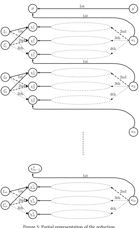
The manipulator will be the only agent owning more than one good. For sake of simplicity, we identify other agents by their goods. Figure 5 describes the preferences of these agents. Solid-line edge denotes the most preferred good, dash-Solid-line edge the second most preferred good, and doted-line edge either the third or fourth most preferred good. Furthermore, the doted-circles are missing goods that will be presented later on. For the time being, we can assume that inner edges and outer edges of these doted-circles are directly connected.
We are now able to present the main idea of the reduction. When the manipulator reveals his true preferences, he obtains his favorite goods except for µ0. Indeed, during ATTC he first exchanges µ with κ1, and then χ11 with ξ1, χ12 with ξ10, χ31 with κ2, and so on. At the end, the manipulator is not able to obtain µ0since he has already exchanged µ with another good. Therefore, he keeps his good χ3
m.
Note that the only way for him to be better of is to obtain his most preferred goods i.e., µ0 instead of χ3
m. But to obtain such assignment, he must exchange • µ with µ0 • χ`i i with κi • χ`0i i with ξi • χ`00i i with ξi0
where for each clause ci, {`i, `0i, `00i} = {1, 2, 3}. The good χ`i exchanged with κiwill correspond to the literal rendering true clause ci. We are now ready to introduce the remaining goods.
The aim of the goods occulted in Figure 5 is to maintain consistency on the choice of literals rendering true clauses. In other words, we want to avoid a situation where two goods χ`
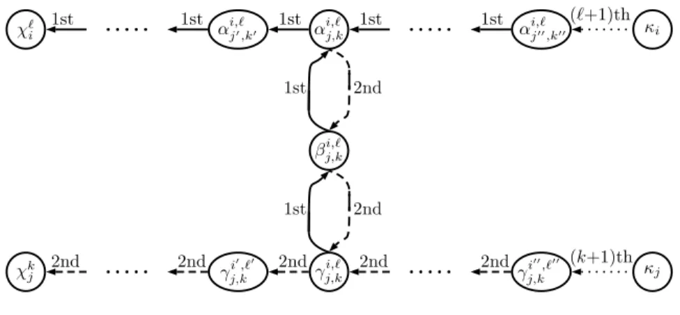
i and χkj, corresponding to a variable and its negation, are exchanged by the manipulator in order to obtain goods κiand κj. To do so, for any pair of literals c`iand ckj, such that c`i is u and ckj is ¬u for some variable u ∈ U, we introduce goods αi,`
j,k, β i,` j,kand γ
i,`
j,k. The preferences of the owners of α i,` j,k, β
i,` j,k and γi,`
j,kare illustrated in Figure 6. In this figure, the most preferred (resp. second most preferred) good for the owner of αi,`
j,k (resp. γ i,` j,k) is α i,` j0,k0 (resp. γ i0,`0 j,k ), where α i,` j0,k0 (resp. γ i0,`0 j,k ) is one of the goods introduced because literal ck0
j0 (resp. c` 0
i0) is ¬u (resp. u) and cj0 (resp. ci0) is the latest clause preceding cj (resp. ck) that contains ¬u (resp. u) as one of its literals. If cj (resp. ci) is the first clause containing ¬u (resp. u) as one of its literals, then the most preferred (resp. second most preferred) good for the owner of αi,`
j,k (resp. γ i,` j,k) is χ
`
i (resp. χkj). Finally, the outgoing edge of κi (resp. κj), which partially appears in Figure 5, is directed toward the (` + 1)th most preferred good (resp. (k + 1)th most preferred good) for the owner of κi(resp. κj). This good is denoted in Figure 5 by αi,` j00,k00(resp. γi 00,`00 j,k ), where α i,` j00,k00(resp. γi 00,`00
j,k ) is one of the good introduced because literal ck00
j00 (resp. c` 00
i00) is ¬u (resp. u) and cj00(resp. ci00) is the last clause that contains ¬u (resp. u) as one of its literals.
To see how this gadget works, assume that the manipulator exchanges χ`
i to obtain κi, corre-sponding to the case where ci is true because of literal c`i (i.e. positive occurrence of variable u). This exchange involves a cycle in the ATTC-graph including the goods on the unique path from κi to χ`i. This path includes good αi,`j,k which is exchanged. The owner of βj,ki,` does not belong to this path, and therefore he keeps his good. Furthermore, the most preferred remaining good for him after this exchange becomes γi,`
j,k. Since β i,`
j,k is the most preferred good for the owner of γj,ki,`, the exchange between these two goods is performed at the next step of ATTC. After this ex-change performed, the unique possible path from κj to χkj is broken and the manipulator cannot use anymore χk
χ1 1 χ2 1 χ3 1 ξ1 ξ1′ χ1 2 χ2 2 χ3 2 ξ2 ξ′ 2 χ1 m χ2 m χ3 m ξm ξ′ m κ1 κ2 χ3 m−1 κm µ 2nd 3th 4th 2nd 3th 4th 2nd 3th 4th 1st 2nd 3th 3th 2nd 1st 3th 2nd 1st 1st 1st 1st 1st κ3 µ′
Figure 5: Partial representation of the reduction
On the other hand, assume now that the manipulator wants to use χk
j to obtain κj, corre-sponding to the case where cj is true because of literal ckj (i.e. negative occurrence of variable u). For this exchange to be possible, it is required for good βi,`
χℓ i α i,ℓ j,k κi βj,ki,ℓ χk j γi,ℓj,k κj (k+1)th 2nd 1st 1st 2nd 2nd (ℓ+1)th 2nd 1st 2nd 1st 1st αi,ℓ j′,k′ 1st 2nd γj,ki′,ℓ′ αi,ℓj′′,k′′ 1st 2nd γj,ki′′,ℓ′′
Figure 6: Goods on the paths from κi to χ`i and from κjto χkj
than γi,`
j,k. But in that case, β i,`
j,k must be exchanged with α i,`
j,k, and thus χ`i cannot be used by the manipulator to obtain κi.
To conclude the proof, we show that there is a truth assignment satisfying all clauses in the M3SAT instance iff there is a beneficial manipulation where the manipulator receives his 3m + 1 most preferred goods. If there is truth assignment Υ satisfying all clauses in the M3SAT instance then we construct a beneficial manipulation step by step as follows. Good µ0 will be at the top of the preference revealed by the manipulator. Thus, the first exchange performed during ATTC will be between µ and µ0. After this exchange performed, the most preferred remaining good for the owner of κ1changes and a path from κ1to χ11appears in the ATTC-graph. If literal c11is true according to Υ then the second good in the preference revealed by the manipulator is κ1, and the third and fourth goods are ξ1 and ξ10, respectively. In that case, κ1 being the most preferred remaining good according to the preference revealed by the manipulator, there is a cycle including χ1
1and the manipulator obtains κ1in exchange of χ11. Afterward, χ21and χ31are exchanged with ξ1 and ξ0
1, respectively. Note that in that case, each good α 1,2
j,k is exchanged with β 1,2
j,k since the most preferred good for the owner of α1,2
j,k is not in the ATTC-graph anymore. For the same reason, αj,k1,3is exchanged with βj,k1,3. On the other hand, if c1
1is not true according to Υ then the second good in the preference revealed by the manipulator is ξ1, and χ11is exchanged with ξ1. Note that in that case, each good α1,1
j,k is exchanged with β 1,1
j,k. Therefore, the second most preferred good for the owner of κ1 is removed from the ATTC-graph, and there is a path from κ1to χ21. In that case, if c2
1 is true according to Υ then the third and fourth goods in the preference revealed by the manipulator are κ1 and ξ10, and both goods are obtained by the manipulator. On the other hand, if literal c2
1 is not true according to Υ then literal c31 is true and the third and fourth goods in the preference revealed by the manipulator are ξ0
1and κ1. We continue in a similar fashion to construct the rest of the preference profile revealed by the manipulator, and it is easy to check that at the end he obtains his 3m + 1 most preferred goods.
Assume now that there is a beneficial manipulation where the manipulator receives his 3m+1 most preferred goods. Note first that µ must be exchanged with µ0. Furthermore, for any clause ci there must be two goods χ`
0
i and χ`
00
i exchanged with goods ξi and ξ0i, because otherwise one of this good will not be obtained by the manipulator. Therefore, the remaining good, say χ`
i, will be the only one available to obtain good κj for a clause cj possibly different to ci. If ciis a clause
containing un-negated variable then χ`
i must be exchanged to obtain κi because otherwise the manipulator will not be able to obtain κi, leading to a contradiction. Indeed, assume by contra-diction that another good, say χk
j is used by the manipulator to obtain κi. By construction, literal ck
j must be a negated occurrence of c`i, because otherwise no path from κi to χkj are possible in the ATTC-graph. But on the other hand, the path from κi to χkj passes through goods α
i,` j,k and βj,ki,`. Therefore, both goods must be part of the remaining goods in the ATTC-graph. Since αi,`j,k is the most preferred good according to the preference of the owner of βi,`
j,k, the path should stop with a cycle including αi,`
j,kand β i,`
j,k, leading to a contradiction. Finally, if ciis a clause containing negated variable then χ`
i must also be exchanged to obtain κi because there is no possible path in the ATTC-graph from κi to a good χkj corresponding to a negated variable. All in all, for each clause ci, there is one good χ`i which is used to obtain κi. Furthermore, by construction we know that no pair of goods χ`
i and χkj, corresponding to a variable and its negation, are exchanged by the manipulator in order to obtain goods κi and κj. Therefore, one can easily construct a truth assignment of the variables in U such that each literal c`
i, corresponding to a good χ`i exchanged with κi, is true. Such assignment satisfies all clauses of C and this concludes the proof.
Appendix C. Basic Properties of ATTC
We compile in this appendix all the basic lemmas which will be of help to prove more elaborate results. We start by providing notations which will be used in all appendices. Consider an assign-ment problem (e, τ ) involving a set of agents or identities N. In this appendix we do not make any hypothesis on the existence of manipulators using multiple identities. These manipulators may or may not exist and all the revealed identities are considered as agents belonging to N. Furthermore, the revealed preference profile τ may or may not contain misreport, and this preference profile, as well as the initial endowment e, are just part of the input of the ATTC procedure.
Let Gk = (Vk, Ek)be the ATTC graph during the step k of ATTC applied to (e, τ ), and let Xk
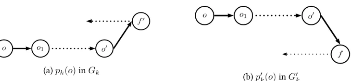
i be the set of goods assigned to agent i after the k first steps. Note that for any step k and for any good o belonging to Vk, there exists a unique directed path in Gk which starts from o and visits various goods of Vk before cycling to one of the goods already visited. Let pk(o)denote this directed path in Gk, and let Sk(o)be the set of goods visited by pk(o). Figure 7a illustrates with solid-line edges such path pk(o1)which could appear in Gk. In this example, the set of goods Sk(o1)visited by pk(o1)is {o1, o2, o4, o5, o6, o7}. The dash-line edges in Figure 7a represents edges of Ekwhich are not part of pk(o1). Figure 7b illustrates with solid-line edges directed path pk(o4) in Gk, which starts from good o4. Note that for any step k of the ATTC procedure and for any good o belonging to Vk, the directed path pk(o)is unique because the outdegree of any vertex in Gkis equal to 1.
It can be seen that the directed path pk(o4)is a subpath of pk(o1)(see Figure 7). More generally, for any good o0 belonging to S
k(o), the directed path pk(o0)is a subpath of pk(o). Furthermore, set Sk(o4)is included in set Sk(o1). Note also that pk(o4)is a cycle containing goods Sk(o4) = {o1, o2, o3, o4}. Therefore pk(o5), pk(o6)and pk(o7)correspond to the same cycle as pk(o4), and Sk(o4) = Sk(o5) = Sk(o6) = Sk(o7)hold.
o3
o1 o2 o4
o5
o6
o7
(a) Oriented path pk(o1)in plain edges
o3
o1 o2 o4
o5
o6
o7
(b) Oriented path pk(o4)in plain edges
Figure 7: Example of ATTC graph Gk
Finally for any good o00 ∈ S
k(o)visited by pk(o), let [pk(o)]o
00
o be the subpath of pk(o)which starts from good o and finishes at good o00. For example, in Figure 7 [p
k(o1)]oo51 is the subpath of pk(o1)which contains edges (o1, o2), (o2, o4)and (o4, o5).
The following lemma states that if the most preferred remaining good for agent i in Gkand Gk+1are the same then no good can be assigned to agent i during step k.
Lemma 3. For any step k ≥ 1 of Algorithm 1, for any good o belonging to Vk and for any good f such that (o, f) belongs to Ek, if f belongs to Vk+1then Xδ(o)k = Xδ(o)k−1.
Proof. Note first that f ∈ Vk+1implies that no cycle including f belongs to Gk. Furthermore, by definition of Algorithm 1 we know that for any good o0belonging to e
δ(o)∩Vk, (o0, f )is the unique outgoing edge from o0 in G
k. Therefore, o0 cannot be visited by a cycle in Gk because otherwise f would be also visited by that cycle. Thus, no good belonging to agent δ(o) is exchanged during step k, and Xk
δ(o) = X k−1 δ(o) holds.
The following lemma shows that if a good labels an ancestor of the current vertex of τiunder consideration during step k then it will also be the case during ulterior steps.
Lemma 4. For any step k ≥ 1 of Algorithm 1 and for any agent i ∈ N, the following inclusion holds: a(τi(Xik−1, X
k−1
i ∪ Vk)) ⊆ a(τi(Xik, Xik∪ Vk+1)). Proof. We know by Lemma 2 that a(τi(Xik−1, X
k−1
i ∪ Vk)) ⊆ K \ Vk. Furthermore, by defi-nition of Algorithm 1 we know that K \ Vk ⊆ K \ Vk+1 and Xik ⊆ K \ Vk+1, implying that Xk
i ⊕ (Xik ∪ Vk+1) = K \ Vk+1. Hence, a(τi(Xik−1, Xik−1 ∪ Vk)) ⊆ Xik ⊕ (Xik ∪ Vk+1) holds. Moreover, by definition of Algorithm 1 we know that Xk−1
i ⊕ (X k−1
i ∪ Vk) = K \ Vk, implying that a(τi(Xik−1, X
k−1
i ∪ Vk)) ⊆ Xik−1 ⊕ (X k−1
i ∪ Vk) holds. On the other hand, K \ Vk ⊆ Xik−1 ⊕ Xik holds since the only good that may differ from Xik−1 to Xik should be part of Vk. All in all, for any o ∈ a(τi(Xik−1, Xik−1 ∪ Vk)), we have o ∈ Xik∪ Vk+1 ⇔ o ∈ Xk
i ⇔ o ∈ X k−1
i ⇔ o ∈ X
k−1
i ∪ Vk. This means that τi(Xik−1), τi(Xik), τi(Xik−1 ∪ Vk)and τi(Xik∪ Vk+1)have in common the subpath from the root to τi(Xik−1, Xik−1∪ Vk), and therefore a(τi(Xik−1, Xik−1∪ Vk)) ⊆ a(τi(Xik, Xik∪ Vk+1))holds.
Corollary 4. For any steps t and r of Algorithm 1 such that r ≥ t and for any agent i ∈ N, the following inclusion holds: a(τi(Xit−1, Xit−1∪ Vt)) ⊆ a(τi(Xir−1, Xir−1∪ Vr)).
The following lemma shows that during any step k, any ancestor of τi(Xik−1, Xik−1 ∪ Vk) which is not assigned to agent i would be preferred by her to any goods of Vk.