Mathematical study and asymptotic analysis of a model for tumor drug resistance

HAL Id: hal-01211770

https://hal.inria.fr/hal-01211770v2

Submitted on 1 Jul 2016

HAL is a multi-disciplinary open access

archive for the deposit and dissemination of

sci-entific research documents, whether they are

pub-lished or not. The documents may come from

teaching and research institutions in France or

L’archive ouverte pluridisciplinaire HAL, est

destinée au dépôt et à la diffusion de documents

scientifiques de niveau recherche, publiés ou non,

émanant des établissements d’enseignement et de

recherche français ou étrangers, des laboratoires

for tumor drug resistance

Thierry Colin, Thomas Michel, Clair Poignard

To cite this version:

Thierry Colin, Thomas Michel, Clair Poignard. Mathematical study and asymptotic analysis of a

model for tumor drug resistance. [Research Report] RR-8784, Inria Bordeaux Sud-Ouest. 2015, 32 p.

�hal-01211770v2�

0249-6399 ISRN INRIA/RR--8784--FR+ENG

RESEARCH

REPORT

N° 8784

Mathematical study and

asymptotic analysis of a

model for tumor drug

resistance

RESEARCH CENTRE BORDEAUX – SUD-OUEST

200 avenue de la Vieille Tour

Thierry Colin

_{, Thomas Michel}

_{, Clair Poignard}

Project-Team MONC

Research Report n° 8784 — October 2015 — 32 pages

Abstract: In this paper we study a partial differential equations model for tumor drug resistance. The aim is to take two different treatments into account: a specific tyrosine kinase inhibitor (TKI) targeted therapy, with a cytotoxic effect, that induces direct cell death, and a multi-targeted TKI, with both cytotoxic and anti-angiogenic effect, which prevents the creation of new blood vessels. The model is based on mass balance equations on cell densities coupled with a diffusion equation for the nutrients and oxygen concentration. We also consider a necrotic phase composed of dead cells, which are eliminated at a rate 1/⌧. We first prove that, for any non-negative ⌧, the model is well-posed and in a second part we study the asymptotic behavior for small ⌧. Such a result is of great interest for the modeling, since it provides a family of ⌧-dependent models which is continuous with respect to ⌧.

Key-words: Tumor growth modeling; partial differential equations; asymptotic analysis.

⇤_{Bordeaux INP, IMB, UMR 5251, F-33400,Talence, France}

†_{INRIA Bordeaux-Sud-Ouest, Team MONC, F-33400, Talence, France} ‡_{Université de Bordeaux, IMB, UMR 5251, F-33400, Talence, France} §_{INRIA Bordeaux-Sud-Ouest, IMB, UMR 5251, F-33400, Talence, France}

Résumé : Dans cet article, nous étudions un modèle d’équations aux dérivées partielles pour la résistance de tumeurs aux traitements. L’objectif de ce modèle est de prendre en compte deux traitements différents. Le premier traitement est une thérapie ciblée inhibitrice de tyrosine kinase (TKI) qui présente un effet cytotoxique, induisant la mort cellulaire. Le second traitement est une thérapie ciblée TKI qui présente à la fois un effet cytotoxique et un effet anti-angiogénique, limitant la création de nouveaux vaisseaux sanguins. Le modèle est basé sur des équations de conservation de la masse pour les densité de cellules, couplées à une équation de diffusion pour la concentration en oxygène et en nutriments. Dans ce modèle, nous considérons également la présence d’une phase de nécrose, composée des cellules mortes et nous supposons que cette nécrose est évacuée à un taux 1/⌧. Dans un premier temps, nous prouvons que pour tout ⌧ strictement positif, le modèle est bien posé. Puis, dans un second temps, nous étudions le comportement asymptotique du modèle quand ⌧ tend vers 0. Le résultat obtenu est intéressant du point de vue de la modélisation, puisqu’il assure l’existence d’une famille de modèles qui est continue par rapport au paramètre ⌧.

Mots-clés : Modélisation de la croissance tumorale, équtions aux dérivées partielles, analyse asymptotique.

Contents

1 Introduction 3

2 The model 5

3 Main results and interpretation 7

4 Preliminary results 10

4.1 Estimates for operator V . . . 11

4.2 Estimates for operators U, N . . . 11

4.3 Estimate for M . . . 18

4.4 Estimates for ⌅ . . . 22

5 Local existence and uniqueness for problems (3) and (4) 22 6 Limit when ⌧ ! 0 25 6.1 Uniform bound on the final time of existence . . . 25

6.2 The limit case ⌧ tends to 0 . . . 30

7 Conclusion 31

1 Introduction

The impact of mathematical modeling in biology has increased dramatically during the last two decades. Particularly in oncology, the increase of biological knowledge combined with the data obtained by invasive and non invasive techniques makes it possible to elaborate more and more accurate models of tumor growth and to study the impact of treatments.

Several kinds of mathematical models for solid tumor growth have been developed over the last few decades. Among them, we can find discrete models or model based on ordinary differential equations (ODE models) or partial differential equations (PDE models). ODE models describe the time evolution of areas or masses of tumors but they account neither for the spatial behavior of the tumor nor for the spatial heterogeneity. Discrete models like cellular automata and agent-based models [10] make it possible to reproduce the growth at the cell-scale but cannot describe the cancer evolution at the organ level. Even though global PDE models at the organ level do not describe the cancer process at the cell scale, they seem adequate for accounting for both time and spatial behavior of the tumor at the macro scale. In this work, we attend to study clinical cases through medical imaging. There is a huge literature concerning the modeling of solid tumor growth with or without treatments and it is impossible to give an extensive list here. However, the reader can refer to [8, 12, 14, 19, 22] for PDE-type models and their mathematical analysis. Models based on reaction-diffusion equations are used to describe the active motion of tumor cells in the case of invasive tumors (see [13] or [20]). Models based on mass balance equations on cell densities are used when the growth is only a consequence of cell proliferation. Roughly speaking, on one hand, primary tumors are composed of degenerate cells of the host organ. These cells are in their original environment and it is hard to determine precisely the boundary of the tumor. On the other hand, metastases are composed of cells that come from a different tissue than the host organ. They are more regular, with sharp interfaces. These interfaces can be described using free boundary methods [17] or multiphase mixtures [7], which consider both cell densities and extracellular matrix [18, 21]. The model we study comes from [4] and is based on mass balance equations. It describes the spatial heterogeneity as a mixture of several cell populations. For

the closure of the model, we assume that the tumor behaves like a fluid in a porous media and we assume Darcy’s law for the velocity field [2]. Other models like visco-elastic laws were also studied in [5]. These models may account for more complex phenomena, but their complexity is too high for clinical applications while Darcy’s law is sufficient as a first approximation to address some clinical cases [9].

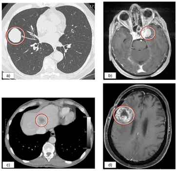
In [15], a model for GIST liver metastases has been studied numerically. This model, based on mass balance equations, enables to explain the tumor evolution observed on clinical images of metastases treated with two targeted therapies. It is well known that mutations will lead to the creation of tumor cells which are resistant to cytotoxic drugs. At the time being, it is not possible to know when such mutations may appear since this may depend on several parameters (such as treatment time, patient variability, external conditions). Therefore, it has been assumed in [15] that different populations of cells co-exist at the initial time of the model. We emphasize that this assumption is meaningful for clinical application since when the tumor is detected, it is very probable that mutations have already occurred. Other models for drug resistance can be studied, by considering that the transition from sensitive to resistant to a treatment is continuous [16]. One of the features of the model of [15] is that it describes the necrosis. Such a necrosis is composed of cells that die because of drugs or hypoxia (the lack of oxygen/nutrients). This necrosis is evacuated at a given rate 1/⌧. Such a necrotic compartment is also important for other kinds of tumors. For example, thyroid metastases to the lung (Figure 1.a) or meningioma (Figure 1.b), in which few necrotic tissue is visible, and glioblastoma (Figure 1.d), a kind of tumor much more aggressive, the parts of which may contain only necrotic tissues. In contrast, compared to these tumors, the necrotic cells of GIST metastases to the liver (Figure 1.c) are more diffuse inside the tumor.

Figure 1: a) metastasis to the lung1_{, b) brain meningioma}2_{, c) GIST metastasis to the liver}1_{, d)}

brain glioma3_.

the well-posedness of the model [15] and to study its asymptotic behavior for small ⌧.

The outline of the paper is the following one. In Section 2 we briefly present the model. The model will be considered in a bounded domain in the case of dimension 2 or 3 in space. Then we present the model without necrosis which will be proved to be the limit model when the necrosis is immediately evacuated. In Section 3 we state the main results. Section 4 is devoted to preliminary results required for Sections 5 and 6. These results use classical estimates for hyperbolic, elliptic and parabolic equations. In Section 5, we prove the well-posedness of the model. The proof is based on a fixed-point method. Finally we perform the asymptotic analysis ⌧ _{! 0 in Section 6. As it will be shown here after, it is a singular perturbation problem. The} interesting fact is that, thanks to our analysis, we can describe the tumor growth evolution under treatment continuously with respect to ⌧.

2 The model

In this section we present the model of Lefebvre et al. provided in [15]. This model describes the evolution of three cancer cell’s populations subjected to two different treatments. The first treatment T1 is a specific tyrosine kinase inhibitor (TKI), which has a cytotoxic effect in clinic.

The second treatment T2is a multi-targeted TKI, with both cytotoxic and anti-angiogenic effect.

P1 stands for the density of the proliferative cells which are assumed to be sensitive to both

treatments T1 and T2, while P2 denotes the density of proliferative cells which are assumed to

be resistant to T1and sensitive to T2. The density of cells that are affected neither by T1 nor T2

are denoted by P3. The nutrient (and oxygen) supply, coming from the healthy tissue, denoted

by M, drives the proliferative rate 1(M ) 2(M )of the three cancer cell species, where 1and 2 are positive functions, standing respectively for the proliferative rate and the death rate due

to hypoxia. In [15], they set

1(M ) =

1 + tanh(R1(M Mhyp))

2 , 2(M ) =

1 tanh(R2(M Mhyp))

2 , (1)

where R1, R2 are coefficients and Mhyp is the hypoxia threshold.

The treatments efficiency is described thanks to the smooth functions of time µ1 and µ2,

which stand for the cytotoxic effect of treatments T1 and T2 respectively. We assume that the

absorption is proportional to the rate of nutrient/oxygen.

When the cells die because of the treatment or hypoxia, they enter to a necrotic phase, whose density is denoted by N. The necrotic compartment is assumed to be evacuated at the rate 1/⌧ where ⌧ is the characteristic evacuation time.

S is the density of the healthy cells, which do not divide, since their metabolism is slow compared to the metabolism of proliferative cells.

The tumor grows at a speed v whose divergence is obtained thanks to the saturation assump-tion:

P1+ P2+ P3+ N + S = 1. (2)

The factor ⇠ is introduced in order to account for the VEGF signal produced by the tumor cells to involve angiogenesis (see [11]). It is assumed to be global at any time and proportional to the number of cells dying by hypoxia, which are the fraction 2(M )

max 2. There exist more complex

1_{Courtesy of J. Palussière, MD at Institut Bergonié, 33000 Bordeaux, France.}

2_{Courtesy of H. Loiseau, MD at Hôpital Pellegrin, CHU Bordeaux, 33000 Bordeaux, France.}

3_{Courtesy of H. M. Fathallah-Shaykh, MD at University of Alabama at Birmingham, Birmingham, AL 35294,} USA.

models of tumor-induced angiogenesis [3]. The smooth function of time ⌫2 stands for the

anti-angiogenic effect of treatment T2and can be for example regularization of the time-characteristic

function of treatment T2. The parameter is the coefficient of absorption of this signal by the

organism.

For further explanations on the model, see [4, 15].

For the sake of clarity, we introduce the following notations, which make it possible to write the problem in a factorized way.

Notation 2.1. For any ↵ 2 Rn_{, 2 R}d _{we denote by}

(↵⌦ )i,j = ↵i j, for i = 1, . . . , n, j = 1, . . . , d,

r · (↵ ⌦ ) = (r · )↵ + ( · r)↵.

The vector u stands for (P1, P2, P3, S)t and we denote by (M) := 1(M ) 2(M ). Now we

define A(M ) := 0 B B @ (M ) (µ1+ µ2)M 0 0 0 0 (M ) µ2M 0 0 0 0 (M ) 0 0 0 0 0 1 C C A, b(M ) := ( 1(M ), 1(M ), 1(M ), 0)t, d(M ) := ( 2(M ) + (µ1+ µ2)M, 2(M ) + µ2M, 2(M ), 0)t, p := (1, 1, 1, 0)t, p1,2:= (1, 1, 0, 0)t, s := (0, 0, 0, 1)t,

and we denote by n the outward normal to ⌦, where ⌦ is a bounded domain in R2 _{or R}3_.

The model of Lefebvre et al. can be written as

@tu +r · (u ⌦ v) = A(M)u, (3a) u = s, if v · n < 0 on @⌦, (3b) @tN +r · (vN) = d(M) · u (1/⌧ )N, (3c) N = 0, if v · n < 0 on @⌦, (3d) r · v = b(M) · u (1/⌧ )N, (3e) v = kr⇧, (3f) ⇧_|@⌦= 0, (3g) @tM M +r · (M⇠r(p · u)) = ⌘Mp · u + C0s· u(1 M ), (3h) M|@⌦= 1, (3i) @t⇠ = ↵ Z ⌦ 2(M ) max 2 (p ⌫2p1,2)· udx ⇠, (3j)

For tumors without necrosis, similar considerations lead to the following model: @tu +r · (u ⌦ v) = A(M)u, (4a) u = s, if v · n < 0 on @⌦, (4b) r · v = (b(M) d(M ))_{· u,} (4c) v = k_r⇧, (4d) ⇧|@⌦= 0, (4e) @tM M +r · (M⇠r(p · u)) = ⌘Mp · u + C0s· u(1 M ), (4f) M|@⌦= 1, (4g) @t⇠ = ↵ Z ⌦ 2(M ) max 2 (p ⌫2p1,2)· udx ⇠. (4h)

Note that we impose homogeneous Dirichlet condition on the pressure ⇧, which implicitly states that the tumor growth has no influence on the tissue far from the tumor location.

3 Main results and interpretation

In this paper we prove the local existence and uniqueness of the solution to the problems (3) and (4), under appropriate assumptions on the initial data and the boundary, as well as the asymptotic behavior of the solution to (3) when ⌧ ! 0.

In our study, we work in a d = 2 or 3 dimensional domain denoted by ⌦. For the spatial regularity, we use the algebra structure of Sobolev space Hs_{(⌦)for s large enough.}

Hypothesis 3.1. Throughout the paper, the following hypothesis hold: • the domain ⌦ is a bounded domain in R2 _{or R}3 _{with C}1 _boundary,

• the rates 1(M )and 2(M )are non-negative and smooth functions (this is the case for the

examples given by (1)),

• the parameters µ1, µ2 and ⌫2 are smooth non-negative functions of time, such as

regular-ization of the time-characteristic functions of treatment T1,T2,

• the parameters k, ⌘, C0, ↵ and are non-negative.

Before stating the Theorems, we introduce the following notations: Notation 3.1. The solution of each equation belongs to specific space:

• for any T > 0, p 2 [1, +1] and s 0, we denote by Lp

T; Hs the space Lp(0, T ; Hs(⌦))

endowed with the norm k'kLp

T;Hs :=k'kLp(0,T ;Hs(⌦)), 8' 2 L p T; H

s_,

for the sake of clarity, for u 2 Lp_{(0, T ; H}s_(⌦))n _{we denote by kuk} Lp

T;Hs the norm of u

components by components,

• for any T > 0, p1, p22 [1, +1] and s1, s2 0, we denote by LpT1; Hs1\ L p2

T ; Hs2 the space

Lp1_{(0, T ; H}s1_{(⌦))\ L}p2_{(0, T ; H}s2_(⌦))endowed with the norm

k'kLp1_T ;Hs1_\LTp2;Hs2 :=k'kLp1_T ;Hs1 +k'kLp2_T ;Hs2, 8' 2 LpT1; Hs1\ L p2 T; Hs2,

• for any s 1, we denote by Es

0 the space Hs(⌦)4⇥ Hs 1(⌦)⇥ R endowed with the norm:

k(u0, M0, ⇠0)kEs

0 :=ku0kHs+kM0kHs 1+|⇠0|, 8(u0, M0, ⇠0)2 E s 0,

• for any T > 0 and s 1, we denote by ETs the space (L1T; Hs)4⇥ L2T; Hs\ L1T; Hs 1⇥

C0_{([0, T ])endowed with the norm:}

k(u, M, ⇠)kEs

T :=kukL1T;Hs+kMkL2T;Hs\L1T;Hs 1+k⇠k1, 8(u, M, ⇠) 2 E s T,

• for any T > 0 and s 0_{, we denote by ET}2,s the space (L2

T; Hs)4⇥ L2T; Hs⇥ L2(0, T )

endowed with the norm: k(u, M, ⇠)kET2,s:=kukL

2

T;Hs+kMkL2T;Hs+k⇠kL2(0,T ), 8(u, M, ⇠) 2 E 2,s T .

Then the local existence and uniqueness result is the following:

Theorem 3.2 (Well-posedness of problems (3) and (4)). Assume the hypotheses 3.1 hold. Let

s 3.

(i) Let ⌧ > 0, (u0, M0, ⇠0)2 E0s and N0 2 Hs(⌦) satisfying the boundary conditions. Let us

assume that the cells densities u0= (P1,0, P2,0, P3,0, S0)t and N0 satisfy

• P1,0, P2,0, P3,0, and N0 are compactly supported in ⌦,

• P1,0, P2,0, P3,0, S0, N0 0,

• P1,0+ P2,0+ P3,0+ N0+ S0= 1.

There exist R k(u0, M0, ⇠0)kEs

0 +kN0kHs and a maximal time of existence T

⌧ _{> 0such}

that the problem (3) has a unique solution ((u, M, ⇠), v, N) in Es

T⌧⇥ L2_T; Hs+1\ L1_T ; Hs⇥

L1

T ; Hs. This solution satisfies

(a) k(u, M, ⇠)kEs

T ⌧ +kNkL1T ⌧;Hs  R,

(b) u, N, v 2 C0_{([0, T}⌧_{]; H}s 1_{(⌦)), M 2 C}0_{([0, T}⌧_{]; H}s 2_{(⌦)), ⇠ 2 C}1_{([0, T}⌧_]),

(c) the cell densities u = (P1, P2, P3, S)t and N satisfy

• for all t < T⌧_{, P}

1(t,·), P2(t,·), P3(t,·), N(t, ·) are compactly supported in ⌦ (i.e

the tumor does not hit the boundary), • P1, P2, P3, S, N 0,

• P1+ P2+ P3+ N + S = 1.

(ii) Let (u0, M0, ⇠0) 2 E0s satisfying the boundary conditions. Let us assume that the cells

densities u0= (P1,0, P2,0, P3,0, S0)tsatisfy

• P1,0, P2,0, P3,0 are compactly supported in ⌦,

• P1,0, P2,0, P3,0, S0 0,

• P1,0+ P2,0+ P3,0+ S0= 1.

There exist R k(u0, M0, ⇠0)kEs

0 and a maximal time of existence T > 0 such that the

problem (4) has a unique solution ((u, M, ⇠), v) in Es

T⇥ L2T; Hs+1\ L1T ; Hs. This solution

satisfies

(a) k(u, M, ⇠)kEs T  R,

(b) u, v 2 C0_{([0, T ]; H}s 1_{(⌦)), M 2 C}0_{([0, T ]; H}s 2_{(⌦)), ⇠ 2 C}1_{([0, T ]),}

(c) the cell densities u = (P1, P2, P3, S)t satisfy

• for all t < T , P1(t,·), P2(t,·), P3(t,·) are compactly supported in ⌦ (i.e the tumor

does not hit the boundary), • P1, P2, P3, S 0,

• P1+ P2+ P3+ S = 1.

Remark 3.1. For the sake of simplicity, we prove the theorem for s integer such that s 3, then interpolation give the result for any real s 3. The only hypothesis needed is that s > d/2 + 1 (which implies that the embedding Hs 1_{(⌦) ,! L}1_{(⌦) is continuous).}

Remark 3.2 (Continuity with respect to initial conditions). Under the assumptions of Theorem 3.2 we have

(i) Let ⌧ > 0. For i = 1, 2, let X0,i:= (u0,i,M0,i, ⇠0,i)2 E0s and N0,i2 Hs(⌦) as in Theorem

3.2 (i) and assume that these initial conditions X0,i, N0,i are bounded by R > 0. Let

((ui, Mi, ⇠i), vi, Ni)be the solution to problem (3) with initial conditions u0,i, M0,i, ⇠0,i and

N0,i. Denote by Xi the vector (ui, Mi, ⇠i). Then there exists CR> 0such that

k(X1, v1, N1) (X2, v2, N2)k2_E2,s 1

T ⌧ ⇥L2T ⌧;Hs⇥L2T ⌧;Hs 1  CRk(X0,1

, N0,1) (X0,2, N0,2)k2_Es 1 0 ⇥Hs 1.

(ii) For i = 1, 2, let X0,i:= (u0,i,M0,i, ⇠0,i)2 E0sas in Theorem 3.2 (ii) and assume that these

initial conditions X0,iare bounded by R > 0. Let ((ui, Mi, ⇠i), vi)be the solution to problem

(4) with initial conditions u0,i, M0,i, ⇠0,i. Denote by Xi the vector (ui, Mi, ⇠i). Then there

exists CR> 0 such that

k(X1, v1) (X2, v2)k2_E2,s 1

T ⌧ ⇥L2T ⌧;Hs  CRkX0,1

X0,2k2_Es 1 0 .

The second result states that, if the initial data are well-prepared, the solution to problem (3) converges to the solution to problem (4) when ⌧ ! 0:

Theorem 3.3 (Asymptotic behavior). For any ⌧ > 0, let u⌧

0, N0⌧, M0⌧ and ⇠0⌧ be as in Theorem

3.2 (i). Let u0, M0 and ⇠0 be as in Theorem 3.2 (ii). Assume that

• lim ⌧!0+ 1 p_⌧kN0⌧kHs = 0, • lim ⌧!0+(u ⌧ 0, M0⌧, ⇠⌧0) = (u0, M0, ⇠0) in E0s 1.

Then there exists T > 0 (independent of ⌧) such that

• for any ⌧ > 0, the problem (3) has a unique solution on [0, T ] denoted by ((u⌧_{, M}⌧_{, ⇠}⌧_{), v}⌧_{, N}⌧₎

and the problem (4) has a unique solution on [0, T ] denoted by ((u, M, ⇠), v), • there exists C > 0 such that for any ⌧ > 0 small enough

1 p_⌧kN⌧kL1 T;Hs+ 1 ⌧kN ⌧ kL2 T;Hs C, • lim ⌧!0+((u ⌧_{, M}⌧_{, ⇠}⌧_{), v}⌧_{) = (u, M, ⇠, v)in E}2,s 1 T ⇥L2T; Hs.

4 Preliminary results

Throughout the paper, we consider d = 2, 3 and s 3. In this section, we prove estimates for the two models we study. The key argument to obtain these estimates is that if the initial data for P1, P2, P3, N have compact support in ⌦, then any solution to (3) or (4) is compactly supported.

One can obtain a priori estimates on the system using non linear estimates in high order Sobolev spaces (similarly to non linear hyperbolic systems, see [1]) and usual parabolic estimates for M. The strategy is therefore to construct a suitable mapping such that this property remains true. In a first step, we start to define the operators which give the solution of each equation and we construct the mappings on which we apply the fixed-point strategy.

Definition 4.1. We consider the following operators • V : f 7 ! v, where v is the solution to

8 < : r · v = f, (in ⌦) v = k_r⇧, (in ⌦) ⇧ = 0, (on @⌦) (5) • U : (u0, v, M )7 ! u, where u is the solution to

8 < : @tu +r · (u ⌦ v) = A(M)u, (in ⌦) u = s, (_{if v · n < 0 on @⌦)} u_|t=0 = u0, (in ⌦) (6) • N : (N0, u0, v, M, ⌧ )7 ! N, where N is the solution to

8 < : @tN +r · (vN) = d(M) · u (1/⌧ )N, (in ⌦) N = 0, (if v · n < 0 on @⌦) N_|t=0 = N0, (in ⌦) (7) with u := U(u0, v, M ).

• M : (M0, u, ⇠)7 ! M, where M is the solution to

8 < :

@tM M +r · (M⇠r(p · u)) = ⌘M p· u + C0s· u(1 M ), (on ⌦)

M|@⌦ = 1,

M_|t=0 = M0,

(8) • ⌅ : (⇠0, u, M )7 ! ⇠, where ⇠ is the solution to

8 < : @t⇠ = ↵ Z ⌦ 2(M ) max 2 (p ⌫2p1,2)· udx ⇠, ⇠_|t=0 = ⇠0. (9) To apply the fixed-point strategy for problem (3), we define the operator as follows: for any X0:= (u0, M0, ⇠0), N0 and X := (u, M, ⇠), N, we define

where ˜X := (˜u, ˜M , ˜⇠)with ˜ u :=U(u0,V(b(M) · u (1/⌧ )N ), M ), ˜ N :=N (N0, u0,V(b(M) · u (1/⌧ )N ), M ), ˜ M :=_M(M0, u, ⇠), ˜ ⇠ := ⌅(⇠0, u, M ),

To apply the fixed-point strategy for problem (4), we define the operator as follows: for any X0:= (u0, M0, ⇠0)and X := (u, M, ⇠), we define

˜ X := (X, X0), where ˜X := (˜u, ˜M , ˜⇠)with ˜ u :=_U(u0,V((b(M) d(M ))· u), M), ˜ M :=_M(M0, u, ⇠), ˜ ⇠ := ⌅(⇠0, u, M ).

In order to prove the well-posedness of problems (3) and (4), we use the facts that • if it exists, the solution to (3) satisfies (X⌧_{, N}⌧_{) = ((X}⌧_{, N}⌧_{), (X}

0, N0), ⌧ ),

• if the solution to (4) exists, it satisfies X = (X, X0).

It is crucial to exhibit the stability and contraction properties of the operators and . Such properties will be deduced after analysis of the operators V, U, N , M and ⌅.

4.1 Estimates for operator V

Since ⌦ is smooth, the following estimates on V are consequences of classical results for linear elliptic equations that can be found in [6]. For the sake of conciseness, the proof of the following property is left to the reader.

Proposition 4.1 (Estimates for V). Let s0 _{ s, p 2 [1, +1] and f 2 L}p T; Hs

0

be given. Then the solution v to (5) belongs to Lp

T; Hs 0₊₁ and satisfies kvk2 LpT;Hs0 +1 Ckfk 2 LpT;Hs0. Moreover, if f 2 C0_{([0, T ]; H}s 2_{(⌦))then v 2 C}0_{([0, T ]; H}s 1_(⌦)).

4.2 Estimates for operators U, N

Let u02 Hs(⌦)4, N02 Hs(⌦), v 2 (L2T; Hs+1)d and M 2 L2T; Hsbe given. We consider u and

N the solutions to (6) and (7). In order to derive explicit formulas for u and N, we use the characteristic method. The difficulty lies in the fact that r · v is not necessarily non-negative and thus we must be able to move forward and backward along the characteristic curves. We use the assumption that u0 s(where s = (0, 0, 0, 1)t) and N0 are compactly supported in ⌦ and

we choose T so that the tumor does not reach the boundary @⌦. More precisely we introduce the following domains:

Definition 4.2. Let ⌦0be an open set compactly embedded in ⌦ and assume that supp(u0 s)[

supp(N0)⇢ ⌦0. For i = 1, 2, 3, we define the open domain ⌦i (see Figure 2) by

⌦i:= x2 ⌦, d(x, ⌦0) < i

4d(@⌦, ⌦0) , for i = 1, 2, 3.

In order to prevent that characteristic curves go out of ⌦ we assume in the following that T is small enough such that

p T_kvkL2

T;Hs+1 <

1

4d(@⌦, ⌦0). (10)

The upper bound (10) on T ensures that

• The characteristic curves are well-defined for any t, t0_{2 [0, T ] and x 2 ⌦} 3 by

⇢

@t0x(t˜ 0, t, x) = v(t0, ˜x(t0, t, x)),

˜

x(t, t, x) = x,

• For i = 0, 1, 2, the characteristic curves coming from ⌦iat t = 0 stay in ⌦i+1for any t  T .

Indeed for any t, t0 _{2 [0, T ] and x 2 ⌦}

2, we have |˜x(t0, t, x) x_{| }p_|t t0_|kvk L2 T;Hs+1 < r |t t0_| T 1 4d(@⌦, ⌦0). ⌦0 ⌦1 ⌦2 ⌦3 ⌦ ⌦0 is such that supp(u0 s)[ supp(N0)⇢⇢ ⌦0, ⌦1 satisfies [ t2[0,T ]

supp(p_{·u(t, ·))[supp(N(t, ·)) ⇢⇢ ⌦}1,

⌦2 is such that u and N have explicit

for-mula in ⌦2 and satisfy

[

t2[0,T ]

supp(u(t,·) s)⇢⇢ ⌦2,

characteristic curves are defined in ⌦3.

Figure 2: The domains defined for the characteristic method

Thanks to the change of coordinates along the characteristic curves, we can come back from ⌦3to ⌦2 and obtain the following explicit formulas for the solutions to (6) and (7) in ⌦2:

8(t, x) 2 [0, T ] ⇥ ⌦2, u(t, x) = exp⇣ Z t 0 (A(M ) r · v)(t0_{, ˜x(t}0_{, t, x))dt}0⌘_u 0(˜x(0, t, x)), (11) N (t, x) = exp⇣ Z t 0 r · v + 1 ⌧ (t 0_{, ˜x(t}0_{, t, x))dt}0⌘_N 0(˜x(0, t, x)) + Z t 0 exp⇣ Z t t0 r · v + 1 ⌧ (t 00_{, ˜x(t}00_{, t, x))dt}00⌘ _{d(M )· u (t}0_{, ˜x(t}0_{, t, x))dt}0_. (12)

This leads to the following property:

Proposition 4.2. Let u02 Hs(⌦)4, N02 Hs(⌦), v 2 (L2T; Hs+1)d and M 2 L2T; Hs. Assume

the 3 following facts:

(i) N0 and the components of u0 are non-negative,

(ii) supp(u0 s)[ supp(N0)is compactly embedded in ⌦0,

(iii) S

t2[0,T ]

supp((_{r · v)(t, ·)) is compactly embedded in ⌦}1.

Then u := U(u0, v, M )and N := N (N0, u0, v, M, ⌧ )satisfy

(i) N and the components of u are non-negative,

(ii) S

t2[0,T ]

⇣

supp(p· u(t, ·)) [ supp(N(t, ·))⌘is compactly embedded in ⌦1,

(iii) S

t2[0,T ]

supp(u(t,·) s)is compactly embedded in ⌦2.

Remark 4.1. The property that S

t2[0,T ]

⇣

supp(p_{· u(t, ·)) [ supp(N(t, ·))}⌘is compactly embedded in ⌦1 implies the 2 followings points:

• S

t2[0,T ]

⇣

supp (_{r · V(b(M) · u} (1/⌧ )N )(t,_·) ⌘is compactly embedded in ⌦1,

• S

t2[0,T ]

⇣

supp (_{r · V((b(M)} d(M ))_{· u)(t, ·)} ⌘is compactly embedded in ⌦1,

which will be useful for the fixed point in Section 5.

Proof. The property that the components of u are non-negative is a consequence of assumption on u0 and explicit formula (11). Then since d(M) · u is non-negative, explicit formula (12) and

assumption on N0 lead to the property that N0is non-negative.

Denote by K0⇢ ⌦0the compact supp(u0 s)[ supp(N0)and denote by K1⇢ ⌦1a compact

such that • S t2[0,T ] ⇣ supp((r · v)(t, ·))⌘⇢ K1, • x 2 ⌦, d(x, K0 1₄d(@⌦, ⌦0) ⇢ K1.

We consider also K2 the compact x 2 ⌦, d(x, K1)1₄d(@⌦, ⌦0) ⇢ ⌦2.

Let us focus on (11). For any t 2 [0, T ] and x 2 ⌦2\ K1, assumption (10) on T ensures that

u0(˜x(0, t, x)) = s. The fact that A(M)s = 0, which implies that exp(A(M))s = s, leads to

u(t, x) = exp⇣ Z

t

0

(r · v)(t0_{, ˜x(t}0_{, t, x))dt}0⌘_{s, for any t 2 [0, T ] and x 2 ⌦}

2\ K1, (13)

and we obtain that p · u(t, ·) = 0 in ⌦2\ K1 for any t 2 [0, T ].

Since ˜x(t0_{, t, x) 2 ⌦ \ K}

1 for any t, t0 2 [0, T ] and x 2 ⌦2\ K2, we deduce from the above

formula that u(t, ·) = s in ⌦2\ K2 for any t 2 [0, T ].

From the explicit expressions for N and u respectively given in (12) and (11), we deduce that d(M )· u(t0_{, ˜x(t}0_{, t, x)) = 0 for any t, t}0_{2 [0, T ] and x 2 ⌦}

2\ K1. Since N0(˜x(0, t, x)) = 0 for any

t2 [0, T ] and x 2 ⌦2\ K1, we conclude that N(t, ·) = 0 in ⌦2\ K1.

In conclusion, the solutions u and N given by the characteristic method in ⌦2 satisfy u = s

and N = 0 in a neighborhood of @⌦2. Thanks to equations (6) and (7), u can be smoothly

extended by u = s in ⌦ \ ⌦2 and N can be smoothly extended by N = 0 in ⌦ \ ⌦2. This

concludes the proof of the Proposition.

The following Lemma gives estimates on @m

xr · (vu)@xmuin terms of kukHm for u 2 Hm(⌦):

Lemma 4.1. Let s0 _{> d/2and K 2 R be given. Let m 2 N such that m  s}0_{. Let v 2 H}s0+1_(⌦).

We assume that u 2 Hm_{(⌦) is such that u = K in a neighborhood of @⌦, therefore @}k

xu|@⌦= 0

for any 1  k  m. Then the following estimate holds: Z

⌦

@mxr · (vu)@xmu  CkvkHs0 +1 K2 m,0+kuk2Hm ,

where m,0 is the Kronecker delta equal to 1 for m = 0 and equal to 0 elsewhere.

Proof. In the proof, we use the Gagliardo-Nirenberg interpolation inequality that can be found in [1]. We start by applying Leibniz formula on the left-hand side

Z ⌦ @xmr · (vu)@xmu  m X k=0 Cmk Z ⌦r · (@ k xv@xm ku)@xmu | {z } =Ik m . • If k = 0, Im0 = Z ⌦r · (v@ m xu)@xmu = Z ⌦ (_{r · v)(@}xmu)2+ Z ⌦ v_·1 2r (@ m xu)2 ,

then integrate by parts the second integral to obtain successively Im0 = Z ⌦ (r · v)(@m xu)2+ 1 2 ✓ K2 m,0 Z @⌦ v· nd Z ⌦ (r · v)(@m xu)2 ◆ , = 1 2 Z ⌦ (_{r · v) K}2 m,0+ (@xmu)2 .

Thanks to the continuous embedding Hs0_{(⌦) ,! L}1_{(⌦) we infer}

• If 1  k  m, Ik mcan be rewritten as Imk = Z ⌦ r · @ k xv @xm ku@mxu | {z } I1 + Z ⌦ @xkv· r @xm ku @xmu | {z } I2 .

Let first estimate I1.

(i) If m 2 and k = m:

|I1|  kr · @xmvkL2kuk_L1k@m_xukL2,

and we use the continuous embedding Hm_,

! L1 _{to obtain}

|I1|  kvkHs0 +1kuk2_Hm.

(ii) Otherwise I1satisfies

|I1|  kr · @kxvkL4k@_xm kuk_L4k@_xmuk_L2,

Gagliardo-Nirenberg inequality and using the fact that s0_{+ 1 3lead to}

|I1|  kvkHs0 +1kuk2_Hm.

Then we focus on I2.

(i) If k = 1:

|I2|  k@xvkL1kr(@_xm 1u)k_L2k@_xmuk_L2,

here again the embedding H2_{(⌦) ,}

! L1_{(⌦) and the fact that s}0_{+ 1 3 lead to}

|I2|  kvkHs0 +1kuk2_Hm.

(ii) Otherwise, for k 2, I2 satisfies

|I2|  k@xkvkL4kr(@_xm ku)k_L4k@_xmuk_L2,

Gagliardo-Nirenberg inequality leads to

|I2|  kvkHs0 +1kuk2_Hm.

The previous Lemma makes it possible to prove the following estimate on the solution to scalar advection equation (14):

Proposition 4.3. Let K 2 R, u0 2 Hs(⌦), v 2 (L2T; Hs+1)d, a, b1, b2 2 L2T; Hs. Let u be a

solution to ₈ < : @tu +r · (vu) = au + b1+ b2, u_|t=0 = u0, u_|@⌦ = K, if v · n < 0 on @⌦ (14) and assume that u = K in a neighborhood of ⌦. Then for all s0_{2 N such that d/2 < s}0_{ s, we}

have kuk2 L1 T;Hs0  ⇣ ku0k2_Hs0 + C p T⇣K2 kvkL2 T;Hs0 +1+kb1kL2T;Hs0 ⌘ +_kb2k2_L2 T;Hs0 ⌘ ⇥ exp⇣CT + CpT (_kvkL2 T;Hs0 +1+kakL2T;Hs0 +kb1kL2T;Hs0) ⌘ . (15)

Remark 4.2. A priori, b1 and b2 play the same role. However for stability of the operator N

and the contraction of U and N , it is important to discriminate their roles. More precisely, the term kb2kL2

T;Hs0 does not appear in the exponential term in (15), which will be crucial in the

following.

Proof. Let m 2 N, m  s0_{, apply the derivative @}m

x to (14), multiply by @xmuand integrate over

⌦. First observe that since Hs0 _{is an algebra, we have}

Z

⌦

@mx(au)@xmu  kaukHs0kuk_Hs0,

 CkakHs0kuk2_Hs0. Then we have Z ⌦ @mxb1@xmu  kb1kHs0kuk_Hs0,  kb1kHs0(1 +kuk2 Hs0), and similarly Z ⌦ @xmb2@xmu  1 2(kb2k 2 Hs0 +kuk 2 Hs0).

By summing the above inequalities, thanks to Lemma 4.1 we obtain straightforwardly @tkuk2_Hs0  C h (1 +kvkHs0 +1+kak_Hs0 +kb1kHs0)kuk2_Hs0 + K2kvkHs0 +1+kb1kHs0 +kb2k2_Hs0 i ,

then integrating between time 0 and t < T and applying Gronwall’s inequality lead to the result.

Thanks Proposition 4.3, we deduce the stability and contraction of the operatorsU and N . Proposition 4.4 (Estimate for U, N ). Operators U and N satisfy the following properties:

(i) (Stability) Let u02 Hs(⌦)4, N02 Hs(⌦), v 2 (L2T; Hs+1)d\(L1T; Hs)dand M 2 L2T; Hs\

L1T ; Hs 1 satisfying the assumptions of Proposition 4.2. Then u := U(u0, v, M )satisfies

kuk2 L1 T;Hs  ⇣ ku0k2Hs+ C p TkvkL2 T;Hs+1 ⌘ exp⇣CpT (kvkL2 T;Hs+1+kMkL2T;Hs) ⌘ , and N := N (N0, u0, v, M, ⌧ )satisfies kNk2 L1 T;Hs  ⇣ kN0k2Hs+ C p T (kvkL2 T;Hs+1+kukL1T;HskMkL2T;Hs) ⌘ exp⇣CpT (kvkL2 T;Hs+1+kukL1T;HskMkL2T;Hs) ⌘ . moreover u, N 2 C0_{([0, T ]; H}s 1_(⌦)).

(ii) (Contraction) For i = 1, 2, let u0,i, N0,i, vi, Mibe as previously and let ui:=U(u0,i, vi, Mi)

and Ni:=N (N0,i, u0,i, vi, Mi, ⌧ ). Assume there exists R > 0 such that

k(ui, Mi, ⇠i)kEs

then we have ku1 u2k2L1 T;Hs 1 CR ⇣ ku0,1 u0,2k2Hs 1 +_kv1 v2k2L2 T;Hs+kM1 M2k 2 L2 T;Hs 1 ⌘ , and kN1 N2k2L1 T;Hs 1  CR ⇣ kN0,1 N0,2k2Hs 1+kv1 v2k2_L2 T;Hs +kM1 M2k2_L2 T;Hs 1+ku1 u2k 2 L2 T;Hs 1 ⌘ . Proof. (i) We apply Proposition 4.3 with s0 _{= s, b}

1 and b2 identically null. For 1  i  4, let

ube the ith _{component of u and a equals to the i}th _{diagonal component of A(M) (recall}

that A(M) is diagonal) and apply Proposition 4.3 to obtain the estimate for u. Apply Proposition 4.3 with s0_{= s, b}

1equals to d(M) · u, a and b2identically null leads to

the estimate for N1_.

To prove the time continuity, the assumptions on v and M and equation (6) imply that @tu

belongs to (L1

T; Hs 1)d. By integrating @tubetween t1and t2 (with 0  t1 t2 T ) and

using the fact that u0 2 Hs(⌦), we obtain that u 2 C0([0, T ]; Hs 1(⌦)) (even Lipschitz

continuous). The same result holds for N.

(ii) Let u1, u2be as in Proposition 4.4, then u1 u2 satisfies the following equation:

@t(u1 u2) +r · ((u1 u2)⌦ v1) = A(M1)(u1 u2)

r · (u2⌦ (v1 v2)) + (A(M1) A(M2))u2.

For 1  i  4, we apply Proposition 4.3 with s0 _{= s 1, v = v}

1, u equals to the ith

component of u1 u2, a equals to the ith diagonal component of A(M1), b1 identically

null and b2 equals to the ith component of r · (u2⌦ (v1 v2)) + (A(M1) A(M2))u2.

Observing that

kr · (u2⌦ (v1 v2))k2Hs 1  ku2⌦ (v1 v2)k2Hs,

 Cku2k2Hskv1 v2k2Hs,

 CRkv1 v2k2Hs,

and integrating between time 0 and T , we obtain kr · (u2⌦ (v1 v2))k2_L2

T;Hs 1  CRkv1 v2k 2 L2

T;Hs.

Similarly, we get the following estimate on A(M1) A(M2):

k(A(M1) A(M2))u2k2L2

T;Hs 1  CRkM1 M2k 2 L2

T;Hs 1.

Then we apply Proposition 4.3 to obtain ku1 u2k2L1 T;Hs 1  ⇣ ku0,1 u0,2k2Hs 1+ CR ⇣ kv1 v2k2L2 T;Hs+kM1 M2k 2 L2 T;Hs 1 ⌘⌘ ⇥ exp⇣CT + CR p T⌘.

1_{Note that the linear term (1/⌧)N in equation (7) is easy to handle: it provides a constant e} t/⌧ _{ 1 for} any 0  t  T .

Finally, since T is bounded by some arbitrary constant, we have proved the estimate on u1 u2.

We use the same ideas to get the estimate on N1 N2.

4.3 Estimate for M

To prove estimates on M, we start to prove estimates on the following equation: 8 < : @tM˜ M +˜ r · (w1M + w˜ 2) = a ˜M + b, ˜ M_|@⌦ = 0, ˜ M_|t=0 = M˜0, (16) where ˜M0 satisfies the boundary condition, w1, w2 and b are compactly supported in ⌦. The

estimates on ˜M make it possible to prove stability and contraction estimates on M. To prove estimate on ˜M, we build ˜M by a Galerkin approximation using the eigenvalues of the operator ( )endowed with the Dirichlet boundary conditions. This makes it possible to assume in the next computations that for any k 2 N, ( )k_{M = 0˜ on the boundary (we can also see this}

from the equation satisfied by ˜M). In order to prove the estimate on ˜M, we need the following Lemma:

Lemma 4.2. Let ˜M02 Hs 1(⌦). Let w12 (L2T; Hs 1)d, a2 L2T; Hs 1 and w22 (L2T; L2)d, b2

L2

T; L2. Assume that ˜M0|@⌦= 0 and that w1, w2 and b are compactly supported in ⌦. Then the

solution ˜M to (16) satisfies

(i) for any k 2 N, such that 2k + 1  s and w22 (L2T; H2k)d, b2 L2T; H2k, we have

@tk( )kM˜k2L2+k( )kr ˜Mk2_L2  C h kw2k2H2k+kbk2_H2k + 1 +_kw1k2Hs 1+kak_H2s 1 k( )kM˜k2_L2 i , (17) (ii) for any k 2 N, such that 2k + 2  s and w22 (L2T; H2k+1)d, b2 L2T; H2k+1, we have

@tk( )kr ˜Mk2L2+k( )k+1M˜k2_L2 C h kw2k2H2k+1+kbk2_H2k+1 + 1 +kw1k2Hs 1+kak_H2s 1 kr( )kM˜k2_L2 i . (18) Proof. We first prove the result for k = 0 since it uses different estimates than general case.

• For k = 0.

To prove (17), multiply the equation (16) by ˜M and integrate by parts: 1 2@tk ˜Mk 2 L2+kr ˜Mk2_L2  Z ⌦ (w1M + w˜ 2)· r ˜M + Z ⌦ (a ˜M + b) ˜M . Using Young’s inequality leads to

1 2@tk ˜Mk 2 L2+kr ˜Mk2_L2  1 2 ⇣ kw1M + w˜ 2)kL22+kr ˜Mk2_L2 +_{ka ˜}M_k2 L2+k ˜Mk2_L2+kbk2_L2+k ˜Mk2_L2 ⌘ ,

then we use the continuous embedding H2_{(⌦) ,}

! L1_{(⌦)for w}

1and get (17) for k = 0.

To prove (18), we apply the operator ( )to (16), multiply by ˜M and integrate by parts: 1 2@tkr ˜Mk 2 L2+k M˜k2_L2 Z ⌦r · (w 1M + w˜ 2)) M +˜ Z ⌦r(a ˜ M + b)_{· r ˜}M . Using Young’s inequality leads to

1 2@tkr ˜Mk 2 L2+k M˜k2_L2  1 2 ⇣ kr · (w1M + w˜ 2))k2L2+k M˜k2_L2 +_{kr(a ˜}M )_k2L2+krbk2_L2+ 2kr ˜Mk2_L2 ⌘ . Observe that kr · (w1M )˜ kL2 k(r · w₁) ˜Mk_L2+kw₁· r ˜Mk_L2,  k(r · w1)kL4k ˜Mk_L4+kw₁· r ˜Mk_L2,

using Gagliardo-Nirenberg inequality for the first term and the continuous embedding H2_{(⌦) ,}

! L1_{(⌦)for the second term leads to}

kr · (w1M )˜ kL2 Ckw₁k_H2kr ˜Mk_L2,

The same idea applied on r(a ˜M )makes it possible to infer kr(a ˜M )kL2 Ckak_H2krMk_L2.

• For k 1.

To prove (17), apply ( )k _{to (16), multiply by ( )}k_{M˜ and integrate by parts:}

1 2@tk( ) k_M k2 L2+k( )krMk2_L2  Z ⌦ ( )k(w1M + w˜ 2))· ( )kr ˜M + Z ⌦ ( )k(a ˜M + b)( )kM .˜ Using Young’s inequality leads to

1 2@tk( ) k_M˜ k2 L2+k( )kr ˜Mk2_L2  1 2 ⇣ k( )k_(w 1M + w˜ 2))k2L2+k( )kr ˜Mk2_L2 +_k( )k_{(a ˜M )} k2 L2+k( )kM˜k2_L2 +_k( )kb_k2L2+k( )kM˜k2_L2 ⌘ , then use the fact that H2k_{(⌦)is an algebra to deduce (17).}

To prove (18), apply ( )k+1 _{to (16), multiply by ( )}k_{M˜ and integrate by parts:}

1 2@tk( ) k r ˜M_k2L2+k( )k+1M˜k2_L2  Z ⌦ ( )k_{r · (w}1M + w˜ 2))( )k+1M˜ + Z ⌦ ( )kr(a ˜M + b)· ( )kr ˜M .

Using Young’s inequality leads to 1 2@tk( ) k r ˜M_k2_L2+k( )k+1M˜k2_L2  1 2 ⇣ k( )k_{r · (w}1M + w˜ 2))kL22+k( )k+1M˜k2_L2 +_k( )k_{r(a ˜}M )_k2_L2+k( )kr ˜Mk2_L2 +k( )krbk2 L2+k( )kr ˜Mk2_L2 ⌘ , then use the fact that H2k+1_{(⌦)is an algebra to obtain (18).}

The previous Lemma leads to the following Proposition, which makes it possible to prove estimates on M:

Proposition 4.5. Under the assumption of Lemma 4.2, for any s0 _{2 N such that s}0 _{ s, we}

have the following estimates k ˜Mk2 L1 T;Hs0 1  ⇣ k ˜M0k2_Hs0 1+ C(kw2k 2 L2 T;Hs0 1+kbk 2 L2 T;Hs0 1) ⌘ ⇥ exphC⇣T +kw1k2_L2 T;Hs 1+kak 2 L2 T;Hs 1 ⌘i . (19) k ˜M_k2 L2 T;Hs0  k ˜M0k 2 Hs0 1+ C h kw2k2_L2 T;Hs0 1+kbk 2 L2 T;Hs0 1 +⇣T +_kw1k2L2 T;Hs 1+kak 2 L2 T;Hs 1 ⌘ k ˜M_k2 L1 T;Hs0 1 i . (20)

Proof. We use Lemma 4.2 and the facts that for k 2 N, k ˜M_kL2+k( )kM˜k_L2 is equivalent to

k ˜M_kH2k and k ˜Mk_L2+k( )kr ˜Mk_L2 is equivalent to k ˜Mk_H2k+1.

• If s0_{= 2m + 1, with m 2 N}⇤_{, we apply (17) for k = 0 and k = m and sum them.}

• If s0_{= 2m + 2, m 2 N}⇤_{, we apply (17) for k = 0 and (18) for k = m and sum them.}

Theses calculations lead to the following estimates: @tk ˜Mk2_Hs0 1+k ˜Mk 2 Hs0  C h kw2k2_Hs0 1+kbk 2 Hs0 1 + 1 +_kw1k2Hs 1+kak2_Hs 1 k ˜Mk2_Hs0 1 i . (21)

We start by omitting the term k ˜M_k2

Hs 0and we integrate between time 0 and t  T . Applying

Gronwall’s inequality leads to (19). To prove (20), we go back to (21), integrate between time 0 and T and omit the term k ˜M (T,_·)k2_Hs0 1.

Now we can prove the main estimates on operator M: Proposition 4.6. Operator M satisfies the following properties:

(i) (Stability) Let M0 2 Hs 1(⌦) such that M0 = 1 on @⌦. Let u 2 (L1T ; Hs)4 such that

p_{· u is compactly supported in ⌦, where p = (0, 0, 0, 1)}t_{. Let ⇠ 2 C}0_{([0, T ]). Then M :=}

M(M0, u, ⇠) satisfies kMk2 L1 T;Hs 1  1 + ⇣ kM0k2Hs 1+ CT (kuk2_L1 T;Hs+k⇠k 2 1) ⌘ ⇥ exphCT⇣1 +kuk2 L1 T;Hs+k⇠k 2 1 ⌘i , kMk2L2 T;Hs 1 + kM0k 2 Hs 1+ CT h kuk2L1 T;Hs+k⇠k 2 1 +⇣1 +_kuk2L1 T;Hs+k⇠k 2 1 ⌘ kMk2L1 T;Hs 1 i . Furthermore M belongs to C0_{([0, T ]; H}s 2_(⌦)).

(ii) (Contraction) For i = 1, 2, let M0,i, ui, ⇠i be as previously and let Mi :=M(M0,i, ui, ⇠i).

Assume there exists R > 0 such that

k(ui, Mi, ⇠i)kEs T  R, then we have kM1 M2k2L2 T;Hs 1  CR ⇣ kM0,1 M0,2k2Hs 2+ku1 u2k2L2 T;Hs 1+k⇠1 ⇠2k 2 L2 T ⌘ . Proof. (i) The proof is a consequence of Proposition 4.5 with s0 _{= sand}

˜ M := 1 M, ˜ M0:= 1 M0, w1:= ⇠r(p · u), w2:= w1, a := (⌘p + C0s)· u, b := ⌘p_{· u.} (ii) We consider ˜ M := M1 M2, ˜ M0:= M0,1 M0,2, w1:= ⇠1r(p · u1), w2:= (⇠1r(p · u1) ⇠2r(p · u2))M2 , a := (⌘p + C0s)· u1, b := (⌘p + C0s)· (u1 u2)M2+ ⌘p· (u1 u2),

and we apply Proposition 4.5 with s0 _{= s 1. Assumptions and equation (19) leads to}

kM1 M2k2L1 T;Hs 2  kM0,1 M0,2k 2 Hs 2+ CR(ku1 u2k2L2 T;Hs 1+k⇠1 ⇠2k 2 L2 T) ⇥ exp(CRT ),

then from (20) we infer kM1 M2k2L2 T;Hs 1  kM0,1 M0,2k 2 Hs 2+ CR h ku1 u2k2L2 T;Hs 1+k⇠1 ⇠2k 2 L2 T + T_kM1 M2k2L1 T;Hs 2 i ,

this ends the proof since T is bounded by some arbitrary constant.

4.4 Estimates for ⌅

Estimates on ⌅ are consequences of Gronwall’s inequality: Proposition 4.7. Operator ⌅ satisfies the following properties:

(i) (Stability) Let ⇠0 2 R. Let u 2 (L1T; Hs)d and M 2 L2T; Hs. Then ⇠ := ⌅(⇠0, u, M )

satisfies k⇠k21 ⇣ |⇠0|2+ CTkuk2L1 T;L1 ⌘ exp(CT ), where C > 0 depends only on ↵, k⌫2k1.

(ii) (Contraction) For i = 1, 2, let ⇠0,i, ui and Mi be as previously and let ⇠i:= ⌅(⇠0,i, ui, Mi).

Assume there exists R > 0 such that

k(ui, Mi, ⇠i)kEs T  R, then we have k⇠1 ⇠2k2₁ CR ⇣ |⇠0,1 ⇠0,2|2+ku1 u2k2_L2 T;L1+kM1 M2k 2 L2 T;L1 ⌘ , where CR> 0 depends only on ↵, k⌫2k1 and R.

Proof. Multiply by ⇠ the equation satisfied by ⇠ and apply Young’s inequality: 1 2@t⇠ 2  C "✓Z ⌦|u| ◆2 + ⇠2 # ⇠2,

integrate over time and apply Gronwall’s inequality to obtain the estimate for ⇠. The estimate for ⇠1 ⇠2follows the same line.

5 Local existence and uniqueness for problems

(3) and (4)

Let us summarize the stability estimates for the operators U, N , V, M and ⌅. Thanks to Propo-sition 4.2 and Remark 4.1, starting from u0 s, N0, p · u, u s and N compactly supported

in ⌦, we observe that the solutions ˜u and ˜N defined by operators or are also compactly supported in ⌦ and stay in the same compact. We get straightforwardly

Proposition 5.1 (Stability estimates for and ). For i = 0, 1, 2, let ⌦i be as in Definition

(i) Let X0:= (u0, M0, ⇠0)2 E0sand N02 Hs(⌦)such that supp(u0 s)[supp(N0)is compactly

embedded in ⌦0.

There exist R kX0kEs

0 +kN0kHs and T ⌧

1 > 0 depending only on R and the parameters

of the model (such as 1, 2, . . .) such that for any X := (u, M, ⇠) 2 ETs⌧

1 and N 2 L 1 T⌧ 1; H s satisfying • S t2[0,T ]

supp(p· u(t, ·)) [ supp(N(t, ·)) is compactly embedded in ⌦1,

• S

t2[0,T ]

supp(u(t,·)) s)is compactly embedded in ⌦2,

• u(t = 0, ·) = u0, N (t = 0,·) = N0, M (t = 0,·) = M0, ⇠(t = 0) = ⇠0, • kXkEs T ⌧₁ +kNkL1T ⌧₁;H s  R, therefore ( ˜X, ˜N ) := ((X, N ), (X0, N0), ⌧ ) satisfies • S t2[0,T ]

supp(p_{· ˜u(t, ·)) [ supp( ˜}N (t,_{·)) is compactly embedded in ⌦}1,

• S

t2[0,T ]

supp(˜u(t,_·)) s)is compactly embedded in ⌦2,

• k ˜X_kEs

T ⌧₁ +k ˜NkL1T ⌧₁;H s  R.

(ii) Let X0:= (u0, M0, ⇠0)2 E0ssuch that supp(u0 s)is compactly embedded in ⌦0.

There exist R kX0kEs

0 and T1> 0depending only on R and the parameters of the model

(such as 1, 2, . . .) such that for any X := (u, M, ⇠) 2 ETs1 satisfying

• S

t2[0,T ]

supp(p_{· u(t, ·)) is compactly embedded in ⌦}1,

• S

t2[0,T ]

supp(u(t,_·)) s)is compactly embedded in ⌦2,

• u(t = 0, ·) = u0, M (t = 0,·) = M0, ⇠(t = 0) = ⇠0,

• kXkEs T1  R,

we deduce that ˜X := (X, X0) satisfies

• S

t2[0,T ]

supp(p_{· ˜u(t, ·)) is compactly embedded in ⌦}1,

• S

t2[0,T ]

supp(˜u(t,_·)) s)is compactly embedded in ⌦2,

• k ˜XkEs T1  R.

Remark 5.1. The final time T⌧

1 dependence on ⌧ is due to (10) and Proposition 4.4 since the

speed defined by satisfies kvkL2 T;Hs+1 C ⇣ kb(M) · ukL2 T;Hs+ 1 ⌧kNkL2T;Hs ⌘ . Then Proposition 4.4 requires that CpT_kvkL2

T;Hs+1 is small enough to obtain

k˜ukL1

Now we summarize the contraction estimates on U, N , M and ⌅:

Proposition 5.2 (Contraction estimates for and ). and satisfy the following contraction estimates:

(i) For i = 1, 2, let X0,i, N0,i, R, T1⌧ and Xi, Ni as in Proposition 5.1 (i) and denote

( ˜X˜i, ˜N˜i) := ( ((Xi, Ni), (X0,i, N0,i), ⌧ ), (X0,i, N0,i), ⌧ ).

Then for all T  T⌧

1, one has k(X˜˜1, ˜N˜1) ( ˜X˜2, ˜N˜2)k2_E2,s 1 T ⇥L 2 T;Hs 1  CR ⇣ k(X0,1, N0,1) (X0,2, N0,2)k2_Es 1 0 ⇥Hs 1 + T_k(X1, N1) (X2, N2)k2_E2,s 1 T ⇥L 2 T;Hs 1 ⌘ . (22) (ii) For i = 1, 2, let X0,i, R, T1 and Xi as in Proposition 5.1 (ii) and denote

˜ ˜

Xi:= ( (Xi, X0,i), X0,i).

Then for all T  T1, one has

kX˜˜1 X˜˜2k2_E2,s 1 T  CR ⇣ kX0,1 X0,2k2_Es 1 0 + TkX1 X2k 2 ET2,s 1 ⌘ . (23)

Therefore, taking X0,1 = X0,2= X0 and N0,1= N0,2= N0 in the previous Proposition leads

to the following result:

Corollary 5.1. Operators and satisfy

(i) Under the assumptions of Proposition 5.1 (i), there exists 0 < T⌧

2  T1⌧ such that

⇤ : (X, N )_{7 ! ((X, N), (X}0, N0), ⌧ ),

is such that ⇤2 _{is a contraction in the set}

E⇤ := n (X, N )2 Es T⌧ 2 ⇥ L 1 T⌧ 2; H s _{such that kXk} Es T ⌧₂ +kNkL1T ⌧₂;Hs R) o endowed with the usual norm on E2,s 1

T⌧ 2 ⇥ L 2 T⌧ 2; H s 1_.

(ii) Under the assumptions of Proposition 5.1 (ii), there exists 0 < T2 T1 such that

⇤ : X_{7 ! (X, X}0),

is such that ⇤2 _{is a contraction in the set}

E⇤ :=

n

(u, M, ⇠)_{2 E}Ts2 such that kXkE_T2s  R)

o endowed with the usual norm on E2,s 1

T2 .

Remark 5.2. The dependence of the final time T⌧

2 on ⌧ is the same as in Proposition 5.1.

Proof of Theorem 3.2. We consider T = T⌧

2 and the set E⇤ endowed with the usual norm

on the Banach space (L2

T; Hs 1)4⇥ L2T; Hs 1⇥ L2(0, T )⇥ L2T; Hs 1. Since the closed unit

ball in L2

T; Hs is compact in the weak topology and the closed unit balls in L1T ; Hs 1 and

in L1

T ; Hs are compact in the weak⇤ topology [6], we get that E⇤ is a closed subspace of

(L2

T; Hs 1)4⇥L2T; Hs 1⇥L2(0, T )⇥L2T; Hs 1. Then we apply the contraction mapping theorem

in E⇤ to obtain the existence and uniqueness of the fixed point (X , N ) 2 E⇤ to ⇤2. Then

applying ⇤ to ⇤2_{(X , N ) = (X , N )leads to the existence and uniqueness of the fixed point}

(X , N )to ⇤ .

Propositions 4.4 and 4.6 lead to the time continuity of u and M stated in Theorem 3.2 (i)b. Then from Propositions 4.1 and 4.7 we infer the time continuity of v and ⇠.

By construction of the solution, we get

P1, P2, P3, N, S 0, where (P1, P2, P3, S)t:= u.

In conclusion, the saturation P1+P2+P3+N +S = 1is a consequence of equation satisfied by

P1+ P2+ P3+ N + Sobtained by summing the equations on P1, P2, P3, N and S and Gronwall’s

inequality.

The exact same reasoning holds for ⇤ .

Remark 5.3. Remark 3.2 is a consequence of Theorem 3.2 and Proposition 5.2, assuming that CRT 1₂ in Proposition 5.2.

6 Limit when ⌧ ! 0

The goal of this section is to prove Theorem 3.3, which is the asymptotic behavior of model (3) for ⌧ ! 0+ _{towards model (4).}

In the previous section, the time of existence T > 0 depends a priori on the norm of v, which depends itself on ⌧ thanks to (3e). More precisely, if we look at the proof of existence, we can see that this time depends only on kvkL2

T;Hs+1. Note that according to Remark 5.1, this norm

could blow up when ⌧ ! 0+_{. Our first goal consists in finding a bound to ensure that the time}

of existence does not depend on ⌧. In the last subsection, we perform the asymptotic analysis to get the convergence of model (3) to model (4).

6.1 Uniform bound on the final time of existence

Let ⌧ > 0 be given. Let u, M, v and N as in Theorem 3.2 (i). According to Remark 5.1, v satisfies kvkL2 T;Hs+1  C ✓ kb(M) · ukL2 T;Hs+ 1 ⌧kNkL2T;Hs ◆ . (24)

The right-hand side blows up as ⌧ ! 0+_{. The goal of the following results is to prove more}

Lemma 6.1. Under the assumptions of Theorem 3.2 (i), N satisfies the following inequality: ✓ 1 p_⌧kNkL1 T;Hs ◆2 + ✓ 1 ⌧kNkL2T;Hs ◆2  CpT ✓ kb(M) · ukL2 T;Hs+ 1 ⌧kNkL2T;Hs ◆ ⇥ ✓ 1 p_⌧kNkL1 T;Hs ◆2 + Ckd(M) · uk2 L2 T;Hs+ ✓ 1 p_⌧kN0kHs ◆2 . (25)

where C does not depend on ⌧.

Proof. We consider the equation satisfied by pN_⌧: @t ✓_N p_⌧ ◆ +_{r ·} ✓ v_pN ⌧ ◆ =d(M )_p · u ⌧ 1 ⌧ ✓_N p_⌧ ◆ , (26)

Let m 2 N such that m  s. Apply @m

x to (26), multiply by @xm(1/

p_{⌧ )N and apply Lemma}

4.1 to @m

xr · (v(1/p⌧ )N )@xm(1/p⌧ )N, sum over m  s and use (24). This leads to

1 2@t ✓ ₁ p ⌧kNkHs ◆2  C ✓ kb(M) · ukHs+ ✓₁ ⌧kNkHs ◆◆ ✓ ₁ p ⌧kNkHs ◆2 + C_{kd(M) · uk}Hs ✓₁ ⌧kNkHs ◆ ₁ ⌧ ✓ ₁ p_⌧kNkHs ◆2 . Applying Young’s inequality, we obtain for almost any time t 2 [0, T ]:

1 2@t ✓ ₁ p_⌧kNkHs ◆2  C ✓ kb(M) · ukHs+ ✓₁ ⌧kNkHs ◆◆ ✓ ₁ p_⌧kNkHs ◆2 +1 2 C 2 kd(M) · uk2 Hs+ 1 ⌧ ✓ ₁ p_⌧kNkHs ◆2! 1 ⌧ ✓ ₁ p_⌧kNkHs ◆2 , then integrate between time 0 and t and take the supremum for t 2 [0, T ] to obtain

✓ ₁ p_⌧kNkL1 T;Hs ◆2 + ✓₁ ⌧kNkL2T;Hs ◆2  C ✓ kb(M) · ukL1 T;Hs+ 1 ⌧kNkL1T;Hs ◆ ⇥ ✓ ₁ p_⌧kNkL1 T;Hs ◆2 + C_{kd(M) · uk}2 L2 T;Hs+ ✓ ₁ p_⌧kN0kHs ◆2 , and estimate the L1

T-norm by the L2T-norm to conclude the proof.

Lemma 6.2. Assume the assumptions of Theorem 3.2 (i) hold. Denote by Y1:=kukL1 T;Hs, Y2:= q kMk2 L1 T;Hs 1+kMk 2 L2 T;Hs, Y3:=k⇠k1, Y4:= q ((1/p⌧ )kNkL1 T;Hs) 2_{+ ((1/⌧ )} kNkL2 T;Hs) 2_.

Then Y := (Y1, Y2, Y3, Y4)satisfies the following estimates

Yi2 F (T, Y), i = 1,· · · , 4, (27) where F1(T, Y) = ⇣ ku0k2Hs+ C p T (Y1Y2+ Y4) ⌘ exp⇣CpT (Y1Y2+ Y4) ⌘ , F2(T, Y) = ⇥1 + kM0k2Hs 1+ CT Y₁2+ Y₃2 exp CT 1 + Y₁2+ Y₃2 ⇤ ⇥⇥1 + CT 1 + Y12+ Y32 ⇤ + 1 +_kM0k2Hs 1+ CT Y₁2+ Y₃2 , F3(T, Y) =|⇠0|2+ CT Y12exp (CT ) , F4(T, Y) = C hp T Y2 4 (Y1Y2+ Y4) + F1(T, Y)2F2(T, Y)2 i + ✓ ₁ p_⌧kN0kHs ◆2 . Proof. The estimates on Y2

1, Y22 and Y32 are simply consequence of stability estimates on U, M

and ⌅ given by Proposition 4.4, 4.6 and 4.7. For the estimates on Y2

4, the estimate (25) leads to

Y42 C hp T Y42(Y1Y2+ Y4) + Y12Y22 i + ✓ 1 p_⌧kN0kHs ◆2 , and we use (27) to bound Y2

1Y22by F1(T, Y)2F2(T, Y)2.

Now we can prove that, for T small enough, Y is uniformly bounded with respect to ⌧. For any R > 0 one has

lim T!0+Fi(T, (R, R, R, R)) = 8 > > > > > < > > > > > : ku0k2Hs, if i = 1, 2(1 +_kM0k2Hs 1), if i = 2, |⇠0|2, if i = 3, ✓ 2Cku0k2Hs(1 +kM0k2Hs 1) + 1 p_⌧kN0kHs ◆2 , if i = 4. Assume there exists C > 0 such that

8⌧ > 0,

✓ ₁

p_⌧kN0kHs

◆2

 C,

then we take R =q2 max ku0k2Hs, 2(1 +kM0k2Hs 1),|⇠0|2, 2Cku0k2Hs(1 +kM0k2Hs 1 + C and

we obtain that there exists T > 0, which depends only on R, such that Y2

i  R2 for 1  i  4.

Proposition 6.1. Assume the assumptions of Theorem 3.2 (i) hold. If there exists C > 0 such that 8⌧ > 0, ku0k2Hs+kM0k2Hs 1+|⇠0|2+ ✓ ₁ p ⌧kN0kHs ◆2  C, then there exists R > 0 and T > 0 such that

8⌧ > 0, ✓ ₁ p_⌧kNkL1 T;Hs ◆2 + ✓₁ ⌧kNkL2T;Hs ◆2  R2_, kuk2 L1 T;Hs R 2_, kMk2 L1 T;Hs 1+kMk 2 L2 T;Hs R 2_, k⇠k2 1 R2.

Therefore the time of existence of the solution to (3) is independent of ⌧.

In order to finish the asymptotic analysis, we also need estimates on the time derivative of u, M, ⇠ and N:

Corollary 6.1. Under the assumptions of Proposition 6.1, there exists CR > 0, such that for

any ⌧ > 0 small enough (i) k@tuk2_L2 T;Hs 1  CR, (ii) k@tMk2_L2 T;Hs 1  CR, (iii) k@t⇠k2₁ CR, (iv) k@tNk2L2 T;Hs 1  CR ⌧ + ✓ ₁ p_⌧kN0kHs ◆2! .

Proof. (i) and (iii) are consequences of equations (3a), (3j) and Proposition 6.1.

To prove (ii), differentiate in time equation (3h) and apply Proposition 4.5 with s0 _{= s 1}

and ˜ M := @tM, ˜ M0:= 0, w1:= ⇠r(p · u), w2:= M @tw1, a := (⌘p + C0s)· u, b := @t(⌘p· u) + M@ta.

Then Proposition 6.1 and previous estimates on @tuand @t⇠leads to (ii).

To prove (iv), we denote by ˜N := @tN, then ˜N satisfies

@tN +˜ r ·

⇣

v ˜N⌘= r · (@tvN ) + @t(d(M )· u) 1

Applying Lemma 4.1 leads to 1 2k ˜Nk 2 Hs 1   C_kvkHs 1 ⌧ k ˜Nk 2 Hs 1+ C (k@tvkHskNk_Hs+k@_t(d(M )· u) k_Hs 1)k ˜Nk_Hs 1,

Thanks to equation (3e) and Proposition 6.1, we have the following estimates kvkL1 T;Hs  CR ✓ 1 +p1_⌧ ◆ , (28)

and for almost any t 2 [0, T ]:

k@tvkHskNk_Hs  C_R ✓ k@t(b(M )· u) kHs 1+ 1 p_⌧k ˜NkHs 1 ◆ , these estimates lead to

1 2k ˜Nk 2 Hs 1   CR ✓ 1 + p1_⌧ ◆ 1 ⌧ k ˜Nk 2 Hs 1 + CR(k@t(b(M )· u) kHs 1+k@_t(d(M )· u) k_Hs 1)k ˜Nk_Hs 1.

Apply Young’s formula to CR(k@t(b(M )· u) kHs 1+k@_t(d(M )· u) k_Hs 1)k ˜Nk_Hs 1, then for ⌧

small enough, ˜N satisfies the following estimate: k ˜N_k2_Hs 1+

1 ⌧k ˜Nk

2

Hs 1 CR k@t(b(M )· u) k2Hs 1+k@t(d(M )· u) k2Hs 1 .

Integrate the previous estimate between time 0 and time t and take the supremum for t 2 [0, T ] to obtain k ˜N_k2_L1 T;Hs 1+ 1 ⌧k ˜Nk 2 L2 T;Hs 1 k ˜N (0,·)k 2 Hs 1 + CR ⇣ k@t(b(M )· u) k2_L2 T;Hs 1+k@t(d(M )· u) k 2 L2 T;Hs 1 ⌘ . Thanks to Proposition 6.1 and previous estimates on @tuand @tM, there exists CR > 0such

that for any ⌧ > 0 small enough k ˜N_k2_L1 T;Hs 1+ 1 ⌧k ˜Nk 2 L2 T;Hs 1  k ˜N (0,·)k 2 Hs 1+ CR. (29)

We focus on the term k ˜N (0,·)k2

Hs 1. Thanks to (3c), ˜N (0,·) satisfies

˜

N (0,_{·) + r · (v(0, ·)N}0) = d(M0)· u0

1 ⌧N0, then we have the following estimate

k ˜N (0,_·)kHs 1 Ckv(0, ·)k_HskN₀k_Hs+ CkM₀k_Hs 1ku₀k_Hs 1+ 1 ⌧kN0kHs 1. Thanks to (28), we have k ˜N (0,_·)k2_Hs 1  CR ✓ 1 + 1 ⌧2kN0k 2 Hs ◆ , then multiply (29) by ⌧ and omit the non-negative term k ˜N_k2

L1 T;Hs 1 to obtain k ˜N_k2 L2 T;Hs 1  CR ✓ ⌧ +1 ⌧kN0k 2 Hs ◆ . (30)

6.2 The limit case ⌧ tends to 0

Proposition 6.1 makes it possible to pass to the limit when ⌧ ! 0+ _{and implies also that N}

converges to 0 in L1

T ; Hs. However the assumption that (1/

p

⌧ )kN0kHs  C is not sufficient

to prove the convergence of the whole solution ((u⌧_{, M}⌧_{, ⇠}⌧_{), v}⌧_{, N}⌧_{). We need to suppose that}

(1/p⌧ )_kN0kHs ! 0 when ⌧ ! 0+ to get Theorem 3.3. Actually the following Lemma ends the

proof of Theorem 3.3:

Lemma 6.3. For any ⌧ > 0, let X⌧

0, N0⌧, X0be as in Theorem 3.2 and Theorem 3.3 and denote

by • (X⌧_{, N}⌧_{)the solution to (X}⌧_{, N}⌧_{) = ((X}⌧_{, N}⌧_{), (X}⌧ 0, N0⌧), ⌧ ), • X the solution to X = (X, X0). Then lim ⌧!0+kX ⌧ _Xk2 ET2,s 1 = 0.

Proof. Assumptions and Proposition 6.1 ensures that there exists R > 0 (depending only on X⌧ 0,

N⌧

0 and X0) such that for any ⌧ > 0, X⌧, (1/⌧)N⌧ and X are bounded by R.

Denote by (u⌧_{, M}⌧_{, ⇠}⌧_{) := X}⌧ _{and by (u, M, ⇠) := X. Remind the contraction estimates on}

U, M and ⌅: ku⌧ u_kL2 T;Hs 1  CRT ⇣ ku⌧0 u0k2Hs 1+kv⌧ vk2_L2 T;Hs+kM ⌧ _M k2L2 T;Hs 1 ⌘ , kM⌧ M_k2_L2 T;Hs 1  CR ⇣ kM0⌧ M0k2Hs 2+ku⌧ uk2_L2 T;Hs 1+k⇠ ⌧ _⇠ k2L2 T ⌘ , k⇠⌧ _⇠ k2 L2 T  CRT ⇣ |⇠⌧ 0 ⇠0|2+ku⌧ uk2_L2 T;L1+kM ⌧ _M k2 L2 T;L1 ⌘ . We need to find an estimate on v⌧ _{v. Observe that}

v⌧ v =V(b(M⌧₎

· u⌧ _{(1/⌧ )N}⌧₎

V((b(M) d(M ))· u),

=_V((b(M⌧) d(M⌧))_{· u}⌧ (b(M ) d(M ))_{· u) + V(d(M}⌧)_{· u}⌧ (1/⌧ )N⌧), then we obtain the following estimate:

kv⌧ _v k2 L2 T;Hs CR ⇣ ku⌧ _u k2 L2 T;Hs 1+kM ⌧ _M k2 L2 T;Hs 1+ " ⌧⌘_, where "⌧ _=kd(M⌧₎ · u⌧ _{(1/⌧ )N}⌧ k2 L2

T;Hs 1. Thanks to Proposition 6.1 and Corollary 6.1 and

using the fact that (1/p⌧ )_kN0kHs ! 0, we obtain

lim ⌧!0+k@tN ⌧ k2 L2 T;Hs 1+kr · (v ⌧_N⌧₎ k2 L2 T;Hs 1= 0,

then equation (3c) ensures that lim

⌧!0+" ⌧_{= 0.}

Making a summary of previous estimates (for M⌧ _{M, use the estimates on u}⌧ _{u and}

⇠⌧ _{⇠to obtain the T term) leads to}

kX⌧ _X k2 E2,s 1 T  CR ⇣ kX⌧ 0 X0k2_Es 1 0 + TkX ⌧ _X k2 E2,s 1 T + " ⌧⌘_,

then we assume that CRT  1₂ to get

kX⌧ X_k2_E2,s 1 T  CR ⇣ kX0⌧ X0k2_Es 1 0 + " ⌧⌘_,

7 Conclusion

A constructive proof of the solution to our model has been derived. The main idea of the proof was that the tumor remains compactly supported in the domain of interest up to a given time. We proved that the minimum time for well-posedness can be bounded independently of the characteristic time ⌧ of necrosis evacuation. This made it possible to prove that our model is consistent with the model without necrosis, which means that the solution to the model without necrosis is given as the limit of solutions for ⌧ goes to 0. This result ensures that our model can describe continuously both situation with or without necrosis.

Acknowledgments

The authors wish to acknowledge Frédéric Lagoutière who started this study. This study has been carried out with financial support from the French State, managed by the French National Research Agency (ANR) in the frame of the "Investments for the future" Programme IdEx Bordeaux - CPU (ANR-10-IDEX-03-02).

References

[1] S. Alinhac and P. Gérard, Pseudo-differential operators and the Nash–Moser theorem, vol. 82, American Mathematical Society, 2007.

[2] D. Ambrosi and L. Preziosi, On the closure of mass balance models for tumor growth, Mathematical Models and Methods in Applied Sciences, 12 (2002), pp. 737–754.

[3] A. R. Anderson and M. Chaplain, Continuous and discrete mathematical models of tumor-induced angiogenesis, Bulletin of mathematical biology, 60 (1998), pp. 857–899. [4] F. Billy, B. Ribba, O. Saut, H. Morre-Trouilhet, T. Colin, D. Bresch,

J.-P. Boissel, E. Grenier, and J.-J.-P. Flandrois, A pharmacologically based multiscale mathematical model of angiogenesis and its use in investigating the efficacy of a new cancer treatment strategy, Journal of theoretical biology, 260 (2009), pp. 545–562.

[5] D. Bresch, T. Colin, E. Grenier, B. Ribba, and O. Saut, A viscoelastic model for avascular tumor growth, research report, 2009.

[6] H. Brezis, Functional analysis, Sobolev spaces and partial differential equations, Springer Science & Business Media, 2010.

[7] H. Byrne and L. Preziosi, Modelling solid tumour growth using the theory of mixtures, Mathematical Medicine and Biology, 20 (2003), pp. 341–366.

[8] H. M. Byrne and M. Chaplain, Growth of necrotic tumors in the presence and absence of inhibitors, Mathematical biosciences, 135 (1996), pp. 187–216.

[9] T. Colin, F. Cornelis, J. Jouganous, J. Palussière, and O. Saut, Patient-specific simulation of tumor growth, response to the treatment, and relapse of a lung metastasis: a clinical case, Journal of Computational Surgery, 2 (2015), pp. 1–17.

[10] D. Drasdo and S. Höhme, Individual-based approaches to birth and death in avascular tumors, Mathematical and Computer Modelling, 37 (2003), pp. 1163–1175.

[11] J. Folkman, Tumor angiogenesis: Therapeutic implications, New England Journal of Medecine, 285 (1971), pp. 1182–1186.

[12] A. Friedman, A hierarchy of cancer models and their mathematical challenges, Discrete and Continuous Dynamical Systems Series B, 4 (2004), pp. 147–160.

[13] R. A. Gatenby and E. T. Gawlinski, A reaction-diffusion model of cancer invasion, Cancer research, 56 (1996), pp. 5745–5753.

[14] T. Hillen, K. J. Painter, and M. Winkler, Convergence of a cancer invasion model to a logistic chemotaxis model, Mathematical Models and Methods in Applied Sciences, 23 (2013), pp. 165–198.

[15] G. Lefebvre, F. Cornelis, P. Cumsille, T. Colin, C. Poignard, and O. Saut, Spatial modelling of tumour drug resistance: the case of gist liver metastases, Mathematical Medicine and Biology, (2016).

[16] A. Lorz, T. Lorenzi, J. Clairambault, A. Escargueil, and B. Perthame, Effects of space structure and combination therapies on phenotypic heterogeneity and drug resistance in solid tumors, arXiv preprint arXiv:1312.6237, (2013).

[17] B. Perthame and N. Vauchelet, Incompressible limit of mechanical model of tumor growth with viscosity, arXiv preprint arXiv:1409.6007, (2014).

[18] L. Preziosi and A. Tosin, Multiphase modelling of tumour growth and extracellular matrix interaction: mathematical tools and applications, Journal of mathematical biology, 58 (2009), pp. 625–656.

[19] T. Saitou, M. Rouzimaimaiti, N. Koshikawa, M. Seiki, K. Ichikawa, and T. Suzuki, Mathematical modeling of invadopodia formation, Journal of theoretical biology, 298 (2012), pp. 138–146.

[20] K. R. Swanson, C. Bridge, J. Murray, and E. C. Alvord, Virtual and real brain tumors: using mathematical modeling to quantify glioma growth and invasion, Journal of the neurological sciences, 216 (2003), pp. 1–10.

[21] A. Tosin, Initial/boundary-value problems of tumor growth within a host tissue, Journal of mathematical biology, 66 (2013), pp. 163–202.

[22] J. P. Ward and J. R. King, Mathematical modelling of drug transport in tumour multicell spheroids and monolayer cultures, Mathematical biosciences, 181 (2003), pp. 177–207.

200 avenue de la Vieille Tour 33405 Talence Cedex

BP 105 - 78153 Le Chesnay Cedex inria.fr