A particle filter to reconstruct a free-surface flow from a depth camera
Texte intégral
Figure


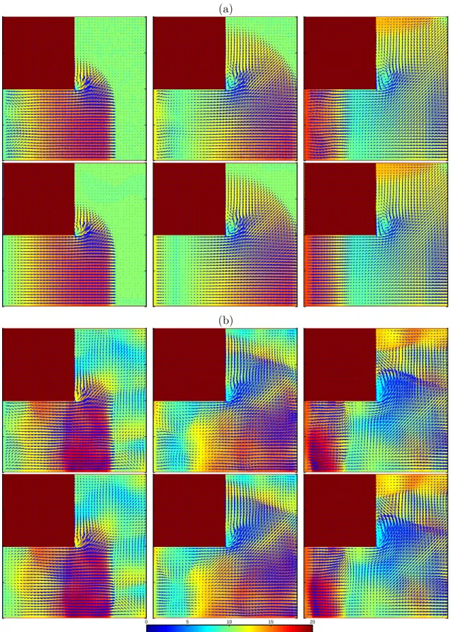
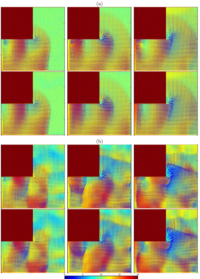
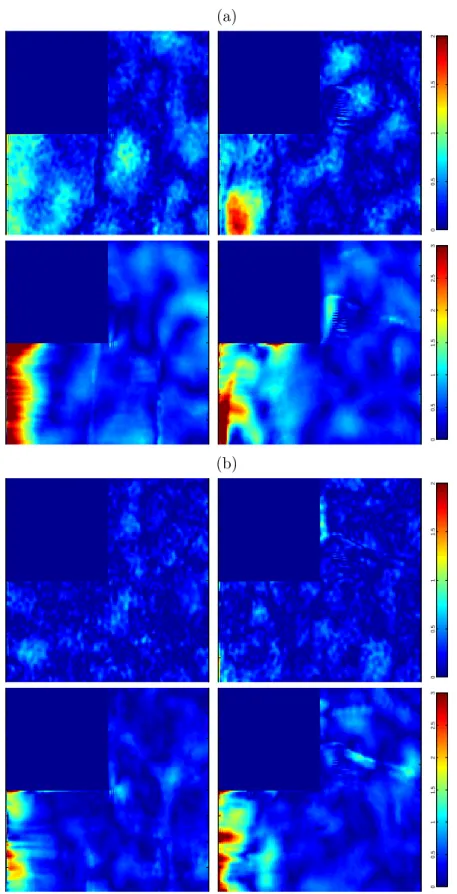
![Figure 5. Error maps for the water column collapse at time t/t 0 = 6.34: (a), with increasing additive noise level σ obs /d 0 ∈ [0.01, 0.04, 0.08]; (b), with increasing perturbations of the initial condition E init ∈ [0.1, 0.2, 0.3]](https://thumb-eu.123doks.com/thumbv2/123doknet/11650871.308475/25.918.137.749.131.1016/figure-collapse-increasing-additive-increasing-perturbations-initial-condition.webp)

Documents relatifs
Based on this generic form of dynamic equation for open branch, we also developed constraint dynamics modeling and numerical algorithm.. The practical applicability in real
OE (right). Both reconstruction methods allowed for a cor- rect identification of zero shifts with a standard deviation σ smaller than 0 .9 mm for almost all scenarios, excepting
The imple- mentation of a multivariate data assimilation scheme faces several challenging issues, which are here addressed and ex- tensively discussed: (1) the effectiveness of
Human Motion Tracking using a Color-Based Particle Filter Driven by Optical Flow.. The 1st International Workshop on Machine Learning for Vision-based Motion Analysis - MLVMA’08,
Using the selected parameters, we compare the tracking error for different motion velocities, motion types, and environment complexities (27 trajectories). 8 presents the results of
We constrain the likely interior structure parameters of the Moon by solving the inverse problem using the observed mass, mean solid MOI, and elastic tidal Love numbers k 2 and h 2
EMSO is the European counterpart to similar large-scale systems in various stages of development around the world (see Favali et al., 2010): United States (Ocean Observatories
Je ne les blâme pas, je préfère les laisser dans leur sentiment de sécurité mais qu'ils sachent que malgré mon apparence forte et mon apparente force, je crie, pleure parfois
